A Second-Order Finite Volume Scheme for Three Dimensional Truncated Pyramidal Quantum Dot

A Second-Order Finite Volume Scheme for

Three Dimensional Truncated Pyramidal

Quantum Dot

Weichung Wang

_{Tsung-Min Hwang}

_{Jia-Chuan Jang}

a_{Department of Applied Mathematics, National University of Kaohsiung,}

Kaohsiung 811, Taiwan. E-mail: [email protected]

b_{Department of Mathematics, National Taiwan Normal University, Taipei 116,}

Taiwan. E-mail: [email protected]

c_{Institute of Applied Mathematics, National Cheng Kung University, Tainan 701,}

Taiwan

Abstract

Three dimensional truncated pyramidal quantum dots are simulated numerically to compute the energy states and the wave functions. The simulation of the hetero-structures is realized by using a novel finite volume scheme to solve the Schr¨odinger equation. The simulation benefits greatly from the finite volume scheme in three-fold. Firstly, the Ben Daniel-Duke hetero-junction interface condition is ingeniously embedded into the scheme. Secondly, the scheme uses uniform meshes in discretiza-tion and leads to simple computer implementadiscretiza-tion. Thirdly, the scheme is efficient as it achieves second order convergence rates over varied mesh sizes. The scheme has successfully computed all the confined energy states and visualized the correspond-ing wave functions. The results further predict the relation of the energy states and wave functions versus the height of the truncated pyramidal quantum dots.

Key words: Three dimensional truncated pyramidal quantum dot, the Schr¨odinger equation, energy levels, wave functions, finite volume scheme, second-order convergence, numerical simulations.

PACS: 02.60.Cb, 03.65.Ge, 73.20.Dx, 73.61. r

1 Introduction

Recent advances in fabrication of semiconductor quantum dots (QD) have attracted many related studies. In this paper, we focus on truncated pyramidal QDs that have been studied intensively in, for example, [3–6,11,12,14–16].

Due to the complicated nature of the Schr¨odinger equation that model the QDs, numerical simulations have played important roles in investigating QDs’ physical properties and applications. However, many of the existed numerical schemes assume that the QDs have simple geometric shapes like cylinder [9,17], cone [10], or pyramid [2,8,13]. Consequently these numerical schemes are not suitable for the truncated pyramidal QDs.

In this paper, we develop simple numerical schemes to simulate three dimen-sional (3D) truncated pyramidal QDs. The schemes allow us to efficiently com-pute all the relevant energy states (eigenvalues of the Schr¨odinger equation) and the corresponding wave functions (eigenvectors) of a 3D truncated pyra-midal QD. The proposed schemes take advantage of the truncated pyrapyra-midal QD geometric structure to embed the truncated pyramidal QD into a Carte-sian coordinate with uniform mesh. The uniform mesh discretization makes the computer implementation much simpler, without sacrificing the accuracy even the wave functions change rapidly around the hetero-junctions. Specif-ically, the numerical experiments show that our numerical schemes achieve a second order accuracy. Furthermore, the schemes choose the mesh points carefully so that the Schr¨odinger equation can be discredited using a finite volume method that automatically builds in the interface conditions. In addi-tion, the Jacobi–Davidson method allows us to efficiently solve the large-scale eigenvalue systems arising in the discretization process.

The rest of the paper is organized as follows. We first describe the truncated pyramidal quantum dot model in Section 2. Then we illustrate the main idea of the finite volume scheme over a 2D trapezoid QD in Section 3. The 3D finite volume discretizations can be generalized straightforwardly, though the pro-cess is quite lengthy. We list the resulting 3D formulas in Appendix. The large scale eigenvalue systems are solved efficiently by the Jacobi–Davidson method that is introduced briefly in Section 3.1. Numerical examples are reported and analyzed in Section 4. Finally we close the paper with a few concluding remarks in Section 5.

2 The model and numerical schemes

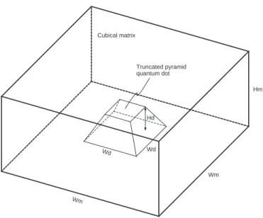
We consider the system that a truncated pyramidal QD is embedded in a cubical matrix. Figure 1 shows the structure schema of the system. The heights of the QD and the matrix are denoted by Hdand Hm, respectively. The widths

of the square bases of the QD and the matrix are denoted by Wd and Wm,

respectively. The governing single-particle Schr¨odinger equation is given by −∇ · (¯h

2

Hd Wd Wd Truncated pyramid quantum dot Cubical matrix Hm Wm Wm

Fig. 1. Structure schema (not in scale) of the system showing that a truncated pyramidal quantum dot is embedded in a cubical matrix.

where ¯h is the reduced Plank constant, λ is the unknown energy state (eigen-value) and u(x, y, z) is the corresponding wave function (eigenvector). The effective electron mass m and confinement potential c are material constants. Therefore they are discontinuous across the hetero-junction. Let

m = ( m1 in the dot, m2 in the matrix, c = ( c1 in the dot, c2 in the matrix. (2)

Associated with the discontinuity in m is the following Ben Daniel-Duke in-terface condition [1] 1 m2 ∂u ∂n ¯ ¯ ¯ ¯ ¯ ∂D+ = 1 m1 ∂u ∂n ¯ ¯ ¯ ¯ ¯ ∂D− , (3)

where D denotes the domain of the truncated pyramidal dot and n represents the normal direction. Note that the + and − signs in D+ and D− denote the

corresponding outward normal derivatives on the interface that are defined for the matrix and the dot regions, respectively. Finally, the Dirichlet boundary conditions

u(xB, yB, zB) = 0 (4)

3 The discretization of the Schr¨odinger equation

We now explain how we discretize the Schr¨odinger equation by the finite vol-ume method. Main ideas for a two dimensional trapezoid (truncated triangle) will be discussed in detail. Lengthy step-by-step exposition of a truncated pyramid will be skipped, as it is simply a straightforward generalization of the 2D case. However, we do provide the resulting 3D discretization formulas in Appendix.

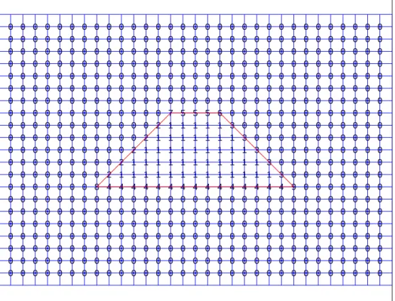
First we define L, M, and N uniform mesh points along the x, y, and z directions, respectively. The mesh points should be chosen properly to fit the interface of the QD in the sense that the no two adjacent mesh points cross the interfaces. See Figure 2 as a 2D mesh scheme example. In the figure, each of the mesh points is labeled by a specific number to identify its location. Furthermore, the mesh sizes are denoted by ∆x, ∆y, and ∆z and the notation

ui,j,k is used to represent the solution of Eq. (1) at the mesh point (xi, yj, zk) =

(i∆x, j∆y, k∆z), for i = 1, · · · , L, j = 1, · · · , M , and k = 1, · · · , N.

The differential operators of the Schr¨odinger equation (1) are then approxi-mated on the chosen mesh points. For the points located in the exterior (label 0 in Figure 2) and interior (label 1) of the QD, we simply apply classical second-order five-point finite differences. For the mesh points that are located on the hetero-junction (labels 2 − 5, 8, and 9), the finite volume schemes described in [8] are applied directly.

Special treatment of the upper corner points (labels 6 and 7) is necessary. Here we present the finite volume method on the upper-right corner point (label 6). The case for the upper-left corner point (label 7) is similar. For clarity and simplicity, we define mo_≡ ¯h2 2m2 and mi _≡ ¯h2 2m1 , (5)

and then rewrite the Schr¨odinger equation (1) and the interface condition (3) as −mef f_{4u + c}ef f_{u = λu (6)} and mo∂u ∂n ¯ ¯ ¯ ¯ ¯ ∂D+ = mi∂u ∂n ¯ ¯ ¯ ¯ ¯ ∂D− , (7) where mef f _{= m}o _{or m}i_{, c}ef f _{= c}o _{or c}i_.

0 0 0 0 0 0 0 0 0 0 0 0 0 0 0 0 0 0 0 0 0 0 0 0 0 0 0 0 0 0 0 0 0 0 0 0 0 0 0 0 0 0 0 0 0 0 0 0 0 0 0 0 0 0 0 0 0 0 0 0 0 0 0 0 0 0 0 0 0 0 0 0 0 0 0 0 0 0 0 0 0 0 0 0 0 0 0 0 0 0 0 0 0 0 0 0 0 0 0 0 0 0 0 0 0 0 0 0 0 0 0 0 0 0 0 0 0 0 0 0 0 0 0 0 0 0 0 0 0 0 0 0 0 0 0 0 0 0 0 0 0 0 0 0 0 0 0 0 0 0 0 0 0 0 8 0 0 0 0 0 0 0 0 0 0 0 0 0 0 0 0 0 0 0 0 4 2 0 0 0 0 0 0 0 0 0 0 0 0 0 0 0 0 0 0 0 4 1 2 0 0 0 0 0 0 0 0 0 0 0 0 0 0 0 0 0 0 4 1 1 2 0 0 0 0 0 0 0 0 0 0 0 0 0 0 0 0 0 4 1 1 1 2 0 0 0 0 0 0 0 0 0 0 0 0 0 0 0 0 4 1 1 1 1 2 0 0 0 0 0 0 0 0 0 0 0 0 0 0 0 4 1 1 1 1 1 7 0 0 0 0 0 0 0 0 0 0 0 0 0 0 4 1 1 1 1 1 5 0 0 0 0 0 0 0 0 0 0 0 0 0 0 4 1 1 1 1 1 5 0 0 0 0 0 0 0 0 0 0 0 0 0 0 4 1 1 1 1 1 5 0 0 0 0 0 0 0 0 0 0 0 0 0 0 4 1 1 1 1 1 6 0 0 0 0 0 0 0 0 0 0 0 0 0 0 4 1 1 1 1 3 0 0 0 0 0 0 0 0 0 0 0 0 0 0 0 4 1 1 1 3 0 0 0 0 0 0 0 0 0 0 0 0 0 0 0 0 4 1 1 3 0 0 0 0 0 0 0 0 0 0 0 0 0 0 0 0 0 4 1 3 0 0 0 0 0 0 0 0 0 0 0 0 0 0 0 0 0 0 4 3 0 0 0 0 0 0 0 0 0 0 0 0 0 0 0 0 0 0 0 9 0 0 0 0 0 0 0 0 0 0 0 0 0 0 0 0 0 0 0 0 0 0 0 0 0 0 0 0 0 0 0 0 0 0 0 0 0 0 0 0 0 0 0 0 0 0 0 0 0 0 0 0 0 0 0 0 0 0 0 0 0 0 0 0 0 0 0 0 0 0 0 0 0 0 0 0 0 0 0 0 0 0 0 0 0 0 0 0 0 0 0 0 0 0 0 0 0 0 0 0 0 0 0 0 0 0 0 0 0 0 0 0 0 0 0 0 0 0 0 0 0 0 0 0 0 0 0 0 0 0 0 0 0 0 0 0 0 0 0 0 0 0 0 0 0 0 0 0 0 0 0 0 0 0 0 0 0 0 0 0

Fig. 2. Uniform mesh scheme of a 2D trapezoid domain. The mesh points in the exterior and interior of the QD are labeled as 0 and 1, respectively. On the het-ero-junction, the left, right, bottom, and upper interfaces are labeled as 2, 3, 4, and 5, respectively. The upper-right, upper-left, lower-left, and lower-right corners are labeled as 6, 7, 8, and 9, respectively.

p q r

Ω

Fig. 3. Discretization schema of the upper-right corners. The solid line represents the hetero-junction. The solid points represent the mesh points.

As shown in Figure 3, we take a rectangle control volume Ω that is centered at the upper right corner mesh point with length in x and y directions be equal to ∆x and ∆y, respectively. We denote the east, north, west, and south boundary of Ω as ∂Ωe, ∂Ωn, ∂Ωw, and ∂Ωs, respectively. By taking the integral

of Eq. (1) and applying the Green’s Theorem, we can rewrite the equation as − ZZ ∇(m∇u) = ZZ (λ − c)u or − Z ∂Ωm ∂u ∂n = ZZ Ω(λ − c)u. (8)

It is clear that the integrals

−

Z

∂Ωm

∂u ∂n over ∂Ωe, ∂Ωs, and ∂Ωn can be approximated by

− Z ∂Ωe mouxd` = −moui+1,j − ui,j ∆x ∆y + O(∆y 3<sub>),</sub> − Z ∂Ωs miuyd` = −mi ui,j−1− ui,j ∆y ∆x + O(∆x 3_), and − Z ∂Ωn mo_u yd` = −mo ui,j+1− ui,j ∆y ∆x + O(∆x 3_),

respectively. As to the integral over ∂Ωw, we assign three virtual mesh points

p, q, and r as shown in Figure 3. These virtual mesh points are created due to the following reason. The west line integral here crosses both the exterior and interior of the QD and the effective mass function is discontinuous. By dividing ∂Ωw into two segments rq and qp and using the facts that

mou+_y = miu−_y ⇒ mou+_yx= miu−_yx, u− x(p) = u+x(q) + ∆y 2 u + yx(q) + O(∆y2), u+ x(r) = u−x(q) − ∆y 2 u − yx(q) + O(∆y2),

we can derive the west line integral as follows.

Z ∂Ωw m∂u ∂nd`y = Z ∂Ωw muxd`y = Z _p q m o_u xd`y+ Z <sub>q</sub> r m i<sub>u</sub> xd`y =mo à ux(p) + ux(q) 2 ! ∆y 2 + m i à ux(q) + ux(r) 2 ! ∆y 2 + O(∆y 3_{) (midpoint rule)} =mo à ux(q) + ux(p) − ux(q) 2 ! ∆y 2 + m i à ux(q) + ux(r) − ux(q) 2 ! ∆y 2 + O(∆y 3₎ =³mi_{+ m}o´∆y 2 ux(q) + ∆y 2 1 2 ³ mo_u+ yx(q) − miu−yx(q) ´_∆y 2 + O(∆y 3₎ =(m i_{+ m}o_{) ∆y} 2 ux(q) + O(∆y 3₎

becomes − Z ∂Ωm ∂u ∂n = − Z ∂Ωe m∂u ∂n − Z ∂Ωn m∂u ∂n − Z ∂Ωs m∂u ∂n − Z ∂Ωw m∂u ∂n = − moui+1,j− ui,j ∆x ∆y − m oui,j+1− ui,j ∆y ∆x − m iui,j−1− ui,j ∆y ∆x − (mi+ mo) 2 ui−1,j − ui,j ∆x ∆y + O(∆y 3₎ = − mi∆x ∆yui,j−1− (mi_{+ m}o₎ 2 ∆y ∆xui−1,j− m o∆y ∆xui+1,j− m o∆x ∆yui,j+1 + "Ã mo+ m i_{+ m}o 2 ! ∆y ∆x + (m i_{+ m}o₎∆x ∆y # ui,j + O(∆y3). (9)

Furthermore, the right hand side of Eq. (8) becomes

ZZ Ω(λ − c)u = −∆x∆y µ₃ 8c i₊ 5 8c o ¶

ui,j+ ∆x∆yλui,j + O(∆y3) (10)

Eqs. (9) and (10) finally lead to the following finite volume scheme for the upper-righr corner point

− mi 1 ∆y2ui,j−1− mi_{+ m}o 2 1 ∆x2ui−1,j − m o 1 ∆x2ui+1,j − m o 1 ∆y2ui,j+1 + "Ã mo₊mi + mo 2 ! 1 ∆x2 + (m i_{+ m}o₎ 1 ∆y2 + µ₃ 8c i₊5 8c o ¶# ui,j =λui,j (11) or equivalently − 1 ∆x2 " mi_{+ m}o 2 ui−1,j+ Ã mi_{+ m}o 2 + m o ! ui,j + moui+1,j # − 1 ∆y2 h mi_u

i,j−1+ (mi+ mo)ui,j+ moui,j+1

i + µ₃ 8c i₊5 8c o ¶ ui,j =λui,j. (12)

Eq. (12) also suggests that the discretization can be composed by the line average of m and the area average of c over the control cell. The 3D formulas shown in the appendix can be understood in the similar manner.

3.1 The resulting eigenvalue problems

The derivation of the 3D scheme is a straightforward generalization of the 2D scheme discussed above. In the appendix, we present the detailed formulas for all mesh points. The 3D finite volume discretization also leads to the formulas

summarized in the appendix. Combining these formulas suitably results in the linear eigenvalue problem

Au = λu, (13)

where A is a sparse matrix with nonzero entries located in the main diagonal and six off-diagonals. We then apply the Jacobi–Davidson method proposed in [8] to solve Eq. (13). See, for example, [8,7,17] for more discussions on solving the large-scale eigenvalue problems arising in numerical simulation of quantum dots by Jacobi–Davidson methods.

4 Computational results

The algorithms have been implemented by Fortran 90 programming language to conduct numerical experiments. The experiments simulate the QD structure that an InAs QD is embedded in the GaAs cuboid. The experiments aim to explore the validity and convergence rate of the algorithms, to compute all the bounded energy states and the corresponding wave functions, and to predict the effect of truncation volume on energy states.

Following parameters are used in our numerical experiments. The effective mass of InAs and GaAs are 0.024me and 0.067me, respectively. The confining

potential for InAs and GaAs are 0.0 eV and 0.7 eV, respectively. The widths of the QD base (Wd in Figure 1) and the cubical matrix base (Wm) are assumed

to be equal to 12.4 nm and 24.8 nm, respectively. Various truncated QDs whose heights (Hd) ranging between 1.0 nm and 6.2 nm (for non-truncated

pyramid) have been tested. The heights of the matrix layers above the top and below the bottom of the QD are assumed to be the same as the QD height in our numerical experiments. The cubical matrix is partitioned into L, M and N meshes in each of the directions. Since we have imposed homogeneous Dirichlet boundary conditions, the total number of unknowns, or the dimension of the matrices is therefore (L − 1) × (M − 1) × (N − 1).

4.1 Rate of convergence

We first check the convergence behavior of the discretization scheme on various QD geometric shapes. We compute all the bounded state energy levels for various mesh sizes. As mesh refines, the rate of convergence is measured by

log₂ Ã λ(4h)_{− λ}(2h) λ(2h)_{− λ}(h) ! ,

(a) Hd = 5.425 nm (Top 12.5% of the QD in height is truncated.)

L × M × N Mtx. Dim. λ1 Order λ2 and λ3 Order

32 × 32 × 22 21,142 0.40046954 - 0.64225897

-64 × -64 × 46 178,605 0.39358538 - 0.63908903

-128 × -128 × 92 1,467,739 0.39173983 1.8992 0.63821870 1.8648 256 × 256 × 184 11,899,575 0.39126226 1.9503 0.63798732 1.9113

(b) Hd = 4.65 nm (Top 25% of the QD in height is truncated.)

L × M × N Mtx. Dim. λ1 Order λ2 and λ3 Order

32 × 32 × 22 20,181 0.40409936 - 0.64179748

-64 × -64 × 46 170,667 0.39677350 - 0.63859390

-128 × -128 × 92 1,403,223 0.39480384 1.8951 0.63771135 1.8599 256 × 256 × 184 11,379,375 0.39429329 1.9478 0.63747627 1.9085

(c) Hd = 3.10 nm (Top 50% of the QD in height is truncated.)

L × M × N Mtx. Dim. λ1 Order λ2 and λ3 Order

32 × 32 × 22 18,259 0.44652787 - 0.64625396

-64 × -64 × 46 154,791 0.43787284 - 0.64211976

-128 × -128 × 92 1,274,191 0.43554850 1.8967 0.64097974 1.8585 256 × 256 × 184 10,338,975 0.43494660 1.9492 0.64067622 1.9092

(d) Hd = 2.325 nm (Top 62.5% of the QD in height is truncated.)

L × M × N Mtx. Dim. λ1 Order λ2 and λ3 Order

32 × 32 × 22 17,298 0.50050117 - 0.66714411

-64 × -64 × 46 146,853 0.49157018 - 0.66247071

-128 × -128 × 92 1,209,675 0.48917779 1.9004 0.66118667 1.8638 256 × 256 × 184 9,818,775 0.48855876 1.9504 0.66084547 1.9120

Fig. 4. Convergence rates for various truncated pyramidal quantum dots.

For the truncated QDs that Hd = 5.425, 4.65, 3.1, and 2.325 nm, Table 4

shows the matrix dimensions, the approximate eigenvalues (denoted by λ1,

λ2, and λ3), and the corresponding convergence rates. It is clear that our finite volume scheme achieves second order convergence rate for various QD structures. That is the error of the scheme is in O(h2_{). Note that similar} convergence behavior are obtained in our experiments for Hd= 3.875, 1.5500,

and 0.7750 nm, though the results are not shown in the table.

4.2 Effects of truncated volume towards energy levels

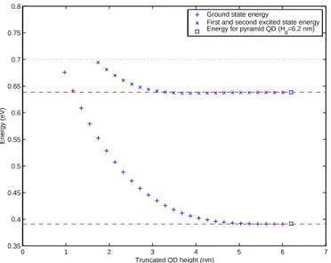
Now we investigate the effect of the truncation volume towards the energy states. Figure 5 shows the energy levels for various truncated QDs. The QD heights rang between 1.0 nm and 6.0 nm. The mesh point numbers (L, M, N ) = (64, 64, 46). Examining the results, we highlight the following observations.

• The energy values increase as the heights of the QDs are decreasing. • The volume of the truncated pyramidal QDs affects the ground state energy

larger than that of the excited state energies. To be specific, for the ground state energy levels, the values changes little (less than 0.002 eV) for QD heights are between 4.84 nm and 6.00 nm. However, for the excited states, the energy values remain similar (with difference less than 0.002 eV) for QD heights are between 3.29 nm and 6.00 nm.

• All the three energy values converge to the energy values corresponding to the pyramid QD reported in [8] (i.e. Hd = 6.2 nm, λ1 = 0.3934 eV and λ2 = λ3 = 0.6391 eV.) Such coincidence shows the validity of the implementation of the schemes for the truncated pyramidal QDs.

4.3 Computational results of wave functions

We finally demonstrate the visualization results of the wave functions. Figure 6 illustrates three dimensional wave functions for Hd = 4.65 nm and 2.325 nm.

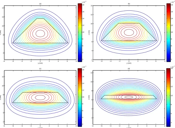
In addition, Figure 7 demonstrates the ground state wave function contours for various truncated QDs in 2D. The contours are plotted on a vertical cross-section passing through the center of the QDs. The figure clearly illustrates how the shapes of the truncated QDs affect the wave functions. In the interior of the QDs, the wave functions are confined by the QDs. In the exterior of the QDs, the contour patterns are basically developed along the shapes of the QD hetero-junctions. We also observe that, as the QD heights becoming smaller, the maximums of the eigenvectors move from the point that is a little higher than the center of the QD to the center of the QD.

5 Conclusion

Aiming at the Schr¨odinger equation modeling the three dimensional truncated pyramidal quantum dots, we have developed a simple yet efficient finite volume scheme to solve the eigenvalue problem numerically. The discretization scheme has been derived in detail, with the discussion of how the induced large scale eigenvalue problems can be solved. Numerical results show that the scheme has successfully solved the Schr¨odinger equation so that we can quantify the energy levels and illustrate the 3D wave functions. The results further verify that the scheme has achieved second order convergence rates numerically for various truncated QD structures. The experiment results have also revealed the effect of how the truncated volume affects the values of energy levels and wave functions. Equipped with the proposed scheme, numerical simulations of other more complicated QD models, e.g. eight-band quantum dot model and vertical aligned QD array, would be possible.

0 1 2 3 4 5 6 7 0.35 0.4 0.45 0.5 0.55 0.6 0.65 0.7 0.75 0.8 Truncated QD height (nm) Energy (eV)

Ground state energy

First and second excited state energy Energy for pyramid QD (H

d=6.2 nm)

Fig. 5. Energy versus heights of the truncated pyramidal quantum dots. The ground state and excited state energy levels for various truncated pyramidal QDs are plot-ted by + and ×, respectively. The first and the second exciplot-ted energy levels have the same values. The dashed lines denote the energies (0.3911 and 0.6380 eV) corre-sponding to the truncated pyramid with Hd = 6.0 nm. The lines are plotted as the

baselines for examining the changes of energies. The energy levels of the pyramid (non-truncated) QD, in which Hd = 6.2 nm, are indicated by the squares.

Acknowledgement

This work is partially supported by the National Science Council and the National Center for Theoretical Sciences in Taiwan.

References

[1] D. J. BenDaniel and C. B. Duke. Space-charge effects on electron tunnelling. Phys. Rev., 152(683), 1966.

[2] D. El-Moghraby, R.G. Johnson, and P. Harrison. Calculating modes of quantum wire and dot systems using a finite differencing technique. Computer Physics Communications, 150:235–246, 2003.

[3] M. De Giorgi, A. Taurino, A. Passaseo, M. Catalano, and R. Cingolani. Interpretation of phase and strain contrast of tem images of InxGa1−xAs/GaAs

quantum dots. Phys. Rev. B, 63:245302, 2001.

[4] M. Hanke, M. Schmidbauer, D. Grigoriev, H. Raidtand P. Sch¨afer, R. K¨ohler, A.-K. Gerlitzke, and H. Wawra. SiGe/Si (001) stranski-krastanow islands by liquid-phase epitaxy: Diffuse x-ray scattering versus growth observations. Phys. Rev. B, 69:075317, 2004.

Fig. 6. Wave functions (eigenvectors) associated with the ground state and the first excited state energies. The heights of QD are equal to 4.65 nm and 2.325 nm for the top and bottom figures.

[5] R. Heitz, F. Guffarth, K. P¨otschke, A. Schliwa, D. Bimberg, N. D. Zakharov, and P. Werner. Shell-like formation of self-organized InAs/GaAs quantum dots. Phys. Rev. B, 71:045325, 2005.

[6] K. D. Hobart, F. J. Kub, H. F. Gray, M. E. Twigg, D. Park, and P. E. Thompson. Growth of low-dimensional structures on nonplanar patterned substrates. Journal of Crystal Growth, 157:338–323, 1995.

[7] T.-M. Hwang, W.-W. Lin, J.-L. Liu, and W. Wang. Jacobi-davidson methods for cubic eigenvalue problems. Numerical Linear Algebra with Applications, To appear.

[8] T.-M. Hwang, W.-W. Lin, W.-C. Wang, and W. Wang. Numerical simulation of three dimensional pyramid quantum dot. Journal of Computational Physics, 196:208–232, 2004.

[9] T.-M. Hwang and W. Wang. Numerical studies of energy states in vertically aligned quantum dot array. Computers and Mathematics with Applications, 49:39–51, 2005.

[10] Y. Li, O. Voskoboynikov, C.P. Lee, and S.M. Sze. Computer simulation of electron energy levels for different shape InAs/GaAs semiconductor quantum dots. Computer Physics Communications, (141):66–72, 2001.

y (nm) z (nm) (a) −8 −6 −4 −2 0 2 4 6 8 4 6 8 10 12 14 2 4 6 8 10 12 14 16 18 x 10−3 y (nm) z (nm) (b) −8 −6 −4 −2 0 2 4 6 8 2 4 6 8 10 12 14 2 4 6 8 10 12 14 16 18 x 10−3 y (nm) z (nm) (c) −8 −6 −4 −2 0 2 4 6 8 2 4 6 8 10 12 2 4 6 8 10 12 14 16 18 x 10−3 y (nm) z (nm) (d) −8 −6 −4 −2 0 2 4 6 8 2 4 6 8 10 12 4 6 8 10 12 14 16 x 10−3

Fig. 7. The ground state wave function contours on the vertical cross-section passing the center of the QDs. The QD boundaries are indicated by the black solid lines. Part (a), (b), (c), and (d) of the figure shows the results for QD heights H_d equal to 5.425, 3.875, 2.325, and 0.775 nm, respectively.

O’Keefe. Atomic structure of defects in GaN:Mg grown with ga polarity. Phys. Rev. Lett., 93(20):206102, 2004.

[12] N. Liu, J. Tersoff, O. Baklenov, Jr. A. L. Holmes, , and C. K. Shih. Nonuniform composition profile in In0.5Ga0.5As alloy quantum dots. Phys. Rev. Lett., 84(2),

2000.

[13] C. Pryor. Quantum wires formed from coupled InAs/GaAs strained quantum dots. Phys. Rev. Lett., 80:3579–3581, 1998.

[14] C. Pryor. Geometry and material parameter dependence of InAs/GaAs quantum dot electronic structure. Phys. Rev. B, 60(4), 1999.

[15] M. Schmidbauer, Th. Wiebach, H. Raidt, M. Hanke, and R. K¨ohler. Ordering of self-assembled Si1−xGex islands studied by grazing incidence small-angle x-ray

scattering and atomic force microscopy. Phys. Rev. B, 58(16), 1998.

[16] F. Silly and M. R. Castell. Selecting the shape of supported metal nanocrystals: Pd huts, hexagons, or pyramids on SrT iO3 (001). Phys. Rev. Lett., 94:046103,

2005.

[17] W. Wang, T.-M. Hwang, W.-W. Lin, and J.-L. Liu. Numerical methods for semiconductor heterostructures with band nonparabolicity. Journal of Computational Physics, 190(1):141–158, 2003.

Appendix: The finite volume formulas for the 3D truncated pyramid

• Points in the exterior of the truncated pyramid: 1

(∆x)2 {m

o_u

i−1,j,k− 2mouijk+ moui+1,j,k}

+ 1

(∆y)2 {m

o_u

i,j−1,k− 2mouijk+ moui,j+1,k}

+ 1

(∆z)2 {m

o_u

i,j,k−1− 2mouijk+ moui,j,k+1}

= couijk− λuijk

• Points in the interior of the truncated pyramid: 1

(∆x)2

n

mi_u

i−1,j,k− 2miuijk+ miui+1,j,k

o

+ 1

(∆y)2

n

miui,j−1,k− 2miuijk+ miui,j+1,k

o

+ 1

(∆z)2

n

miui,j,k−1− 2miuijk+ miui,j,k+1

o

= ci_u

ijk− λuijk

• Points on the western surface of the truncated pyramid: 1 (∆x)2 n mo_u i−1,j,k− ³ mi_{+ m}o´_u ijk+ miui+1,j,k o + 1 (∆y)2 ( mi_{+ m}o

2 (ui,j−1,k− 2uijk+ ui,j+1,k)

) + 1 (∆z)2 n miui,j,k−1− ³ mo+ mi´uijk+ moui,j,k+1 o = ci+ co

2 uijk− λuijk

• Points on the eastern surface of the truncated pyramid: 1 (∆x)2 n mi_u i−1,j,k− ³ mi _{+ m}o´_u ijk+ moui+1,j,k o + 1 (∆y)2 ( mi_{+ m}o

2 (ui,j−1,k− 2uijk+ ui,j+1,k)

) + 1 (∆z)2 n mi_u i,j,k−1− ³ mo_{+ m}i´_u ijk+ moui,j,k+1 o = ci+ co

• Points on the northern surface of the truncated pyramid: 1

(∆x)2

(

mi_{+ m}o

2 (ui−1,j,k− 2uijk+ ui+1,j,k)

) + 1 (∆y)2 n mi_u i,j−1,k− ³ mi_{+ m}o´_u ijk+ moui,j+1,k o + 1 (∆z)2 n mi_u i,j,k−1− ³ mi_{+ m}o´_u ijk+ moui,j,k+1 o = ci+ co

2 uijk− λuijk

• Points on the southern surface of the truncated pyramid: 1

(∆x)2

(

mi_{+ m}o

2 (ui−1,j,k− 2uijk+ ui+1,j,k)

) + 1 (∆y)2 n mo_u i,j−1,k− ³ mi_{+ m}o´_u ijk+ miui,j+1,k o + 1 (∆z)2 n mi_u i,j,k−1− ³ mi_{+ m}o´_u ijk+ moui,j,k+1 o = c i_{+ c}o

2 uijk− λuijk

• Points on the bottom surface of the truncated pyramid: 1

(∆x)2

(

mi_{+ m}o

2 (ui−1,j,k− 2uijk+ ui+1,j,k)

)

+ 1

(∆y)2

(

mi_{+ m}o

2 (ui,j−1,k− 2uijk+ ui,j+1,k)

) + 1 (∆z)2 n mo_u i,j,k−1− ³ mi_{+ m}o´_u ijk+ miui,j,k+1 o = c i_{+ c}o

2 uijk− λuijk

• Points on the southwestern edge of the truncated pyramid: 1 (∆x)2 ( mo_u i−1,j,k − Ã mo₊mi + mo 2 ! uijk+ mi_{+ m}o 2 ui+1,j,k ) + 1 (∆y)2 ( mo_u i,j−1,k− Ã mo₊mi+ mo 2 ! uijk+ mi_{+ m}o 2 ui,j+1,k ) + 1 (∆z)2 n mi_u i,j,k−1− ³ mi_{+ m}o´_u ijk+ moui,j,k+1 o = ci+ 2co

• Points on the southeastern edge of the truncated pyramid: 1 (∆x)2 ( mi_{+ m}o 2 ui−1,j,k− Ã mo₊ mi+ mo 2 ! uijk+ moui+1,j,k ) + 1 (∆y)2 ( mo_u i,j−1,k− Ã mo₊mi+ mo 2 ! uijk+ mi_{+ m}o 2 ui,j+1,k ) + 1 (∆z)2 n mi_u i,j,k−1− ³ mi_{+ m}o´_u ijk+ moui,j,k+1 o = ci+ 2co

3 uijk− λuijk

• Points on the northwestern edge of the truncated pyramid: 1 (∆x)2 ( moui−1,j,k − Ã mo+m i _{+ m}o 2 ! uijk+ mi_{+ m}o 2 ui+1,j,k ) + 1 (∆y)2 ( mi_{+ m}o 2 ui,j−1,k − Ã mo₊mi+ mo 2 ! uijk+ moui,j+1,k ) + 1 (∆z)2 n mi_u i,j,k−1− ³ mi_{+ m}o´_u ijk+ moui,j,k+1 o = c i_{+ 2c}o

3 uijk− λuijk

• Points on the northeastern edge of the truncated pyramid: 1 (∆x)2 ( mi_{+ m}o 2 ui−1,j,k− Ã mo₊ mi+ mo 2 ! uijk+ moui+1,j,k ) + 1 (∆y)2 ( mi_{+ m}o 2 ui,j−1,k − Ã mo+m i_{+ m}o 2 ! uijk+ moui,j+1,k ) + 1 (∆z)2 n miui,j,k−1− ³ mi+ mo´uijk+ moui,j,k+1 o = ci+ 2co

3 uijk− λuijk

• Points on the western edge at the bottom of the truncated pyramid: 1 (∆x)2 ( mo_u i−1,j,k − Ã mo₊mi + mo 2 ! uijk+ mi_{+ m}o 2 ui+1,j,k ) + 1 (∆y)2 ( mi_{+ 7m}o

8 (ui,j−1,k− 2uijk+ ui,j+1,k)

)

+ 1

(∆z)2 {m

o_u

i,j,k−1− 2mouijk+ moui,j,k+1}

= ci+ 7co

• Points on the eastern edge at the bottom of the truncated pyramid: 1 (∆x)2 ( mi_{+ m}o 2 ui−1,j,k− Ã mo₊ mi+ mo 2 ! uijk+ moui+1,j,k ) + 1 (∆y)2 ( mi_{+ 7m}o

8 (ui,j−1,k− 2uijk+ ui,j+1,k)

)

+ 1

(∆z)2 {m

o_u

i,j,k−1− 2mouijk+ moui,j,k+1}

= ci+ 7co

8 uijk− λuijk

• Points on the southern edge at the bottom of the truncated pyramid: 1

(∆x)2

(

mi_{+ 7m}o

8 (ui−1,j,k − 2uijk+ ui+1,j,k)

) + 1 (∆y)2 ( mo_u i,j−1,k− Ã mo₊ mi+ mo 2 ! uijk+ mi_{+ m}o 2 ui,j+1,k ) + 1 (∆z)2 {m o_u

i,j,k−1− 2mouijk+ moui,j,k+1}

= c

i_{+ 7c}o

8 uijk− λuijk

• Points on the northern edge at the bottom of the truncated pyramid: 1

(∆x)2

(

mi_{+ 7m}o

8 (ui−1,j,k − 2uijk+ ui+1,j,k)

) + 1 (∆y)2 ( mi_{+ m}o 2 ui,j−1,k− Ã mo+ m i_{+ m}o 2 ! uijk+ moui,j+1,k ) + 1 (∆z)2 {m o_u

i,j,k−1− 2mouijk+ moui,j,k+1}

= ci+ 7co

8 uijk− λuijk

• The southwestern corner at the bottom of the truncated pyramid: 1 (∆x)2 ( mo_u i−1,j,k− Ã mo₊mi+ 7mo 8 ! uijk+ mi_{+ 7m}o 8 ui+1,j,k ) + 1 (∆y)2 ( mo_u i,j−1,k− Ã mo₊ mi+ 7mo 8 ! uijk+ mi_{+ 7m}o 8 ui,j+1,k ) + 1 (∆z)2{m o_u

i,j,k−1− 2mouijk+ moui,j,k+1}

= ci+ 23co

• The southeastern corner at the bottom of the truncated pyramid: 1 (∆x)2 ( mi _{+ 7m}o 8 ui−1,j,k− Ã mo₊ mi+ 7mo 8 ! uijk+ moui+1,j,k ) + 1 (∆y)2 ( mo_u i,j−1,k− Ã mo₊ mi+ 7mo 8 ! uijk+ mi_{+ 7m}o 8 ui,j+1,k ) + 1 (∆z)2{m o_u

i,j,k−1− 2mouijk+ moui,j,k+1}

= ci+ 23co

24 uijk− λuijk

• The northwestern corner at the bottom of the truncated pyramid: 1 (∆x)2 ( moui−1,j,k− Ã mo+m i_{+ 7m}o 8 ! uijk+ mi_{+ 7m}o 8 ui+1,j,k ) + 1 (∆y)2 ( mi_{+ 7m}o 8 ui,j−1,k − Ã mo₊mi+ 7mo 8 ! uijk+ moui,j+1,k ) + 1 (∆z)2{m o_u

i,j,k−1− 2mouijk+ moui,j,k+1}

= c

i_{+ 23c}o

24 uijk− λuijk

• The northeastern corner at the bottom of the truncated pyramid: 1 (∆x)2 ( mi _{+ 7m}o 8 ui−1,j,k− Ã mo₊ mi+ 7mo 8 ! uijk+ moui+1,j,k ) + 1 (∆y)2 ( mi_{+ 7m}o 8 ui,j−1,k − Ã mo+m i_{+ 7m}o 8 ! uijk+ moui,j+1,k ) + 1 (∆z)2{m o_u

i,j,k−1− 2mouijk+ moui,j,k+1}

= ci+ 23co

24 uijk− λuijk

• Points on the upper bottom surface of the truncated pyramid: 1

(∆x)2

(

mi_{+ m}o

2 (ui−1,j,k− 2uijk+ ui+1,j,k)

)

+ 1

(∆y)2

(

mi_{+ m}o

2 (ui,j−1,k− 2uijk+ ui,j+1,k)

) + 1 (∆z)2 n mi_u i,j,k−1− ³ mi_{+ m}o´_u ijk+ moui,j,k+1 o = ci+ co

• The northwestern corner at the upper bottom of the truncated pyramid: 1 (∆x)2 ( mo_u i−1,j,k− Ã mo₊ 3mi+ 5mo 8 ! uijk+ 3mi _{+ 5m}o 8 ui+1,j,k ) + 1 (∆y)2 ( 3mi_{+ 5m}o 8 ui,j−1,k − Ã mo₊3mi+ 5mo 8 ! uijk+ moui,j+1,k ) + 1 (∆z)2 n mi_u i,j,k−1− ³ mi_{+ m}o´_u ijk+ moui,j,k+1 o = 7ci+ 17co

24 uijk− λuijk

• The southwestern corner at the upper bottom of the truncated pyramid: 1 (∆x)2 ( moui−1,j,k− Ã mo+ 3m i_{+ 5m}o 8 ! uijk+ 3mi _{+ 5m}o 8 ui+1,j,k ) + 1 (∆y)2 ( mo_u i,j−1,k− Ã mo₊ 3mi+ 5mo 8 ! uijk+ 3mi_{+ 5m}o 8 ui,j+1,k ) + 1 (∆z)2 n mi_u i,j,k−1− ³ mi_{+ m}o´_u ijk+ moui,j,k+1 o = 7c i_{+ 17c}o

24 uijk− λuijk

• The northeastern corner at the upper bottom of the truncated pyramid: 1 (∆x)2 ( 3mi _{+ 5m}o 8 ui−1,j,k− Ã mo₊ 3mi+ 5mo 8 ! uijk+ moui+1,j,k ) + 1 (∆y)2 ( 3mi_{+ 5m}o 8 ui,j−1,k − Ã mo+3m i_{+ 5m}o 8 ! uijk+ moui,j+1,k ) + 1 (∆z)2 n miui,j,k−1− ³ mi+ mo´uijk+ moui,j,k+1 o = 7ci+ 17co

24 uijk− λuijk

• The southeastern corner at the upper bottom of the truncated pyramid: 1 (∆x)2 ( 3mi _{+ 5m}o 8 ui−1,j,k− Ã mo₊ 3mi+ 5mo 8 ! uijk+ moui+1,j,k ) + 1 (∆y)2 ( mo_u i,j−1,k− Ã mo₊ 3mi+ 5mo 8 ! uijk+ 3mi_{+ 5m}o 8 ui,j+1,k ) + 1 (∆z)2 n mi_u i,j,k−1− ³ mi_{+ m}o´_u ijk+ moui,j,k+1 o = 7ci+ 17co

• Points on the northern edge at the upper bottom of the truncated pyramid: 1

(∆x)2

(

3mi_{+ 5m}o

8 (ui−1,j,k− 2uijk+ ui+1,j,k)

) + 1 (∆y)2 ( mi_{+ m}o 2 ui,j−1,k− Ã mo₊ mi+ mo 2 ! uijk+ moui,j+1,k ) + 1 (∆z)2 n mi_u

i,j,k−1− (mi+ mo)uijk+ moui,j,k+1

o

= 3c

i_{+ 5c}o

8 uijk− λuijk

• Points on the southern edge at the upper bottom of the truncated pyramid: 1

(∆x)2

(

3mi_{+ 5m}o

8 (ui−1,j,k− 2uijk+ ui+1,j,k)

) + 1 (∆y)2 ( mo_u i,j−1,k− Ã mo₊ mi+ mo 2 ! uijk+ mi_{+ m}o 2 ui,j+1,k ) + 1 (∆z)2 n mi_u

i,j,k−1− (mi+ mo)uijk+ moui,j,k+1

o

= 3ci+ 5co

8 uijk− λuijk

• Points on the western edge at the upper bottom of the truncated pyramid: 1 (∆x)2 ( mo_u i−1,j,k − Ã mo₊mi + mo 2 ! uijk+ mi_{+ m}o 2 ui+1,j,k ) + 1 (∆y)2 ( 3mi_{+ 5m}o

8 (ui,j−1,k− 2uijk+ ui,j+1,k)

)

+ 1

(∆z)2

n

miui,j,k−1− (mi+ mo)uijk+ moui,j,k+1

o

= 3ci+ 5co

8 uijk− λuijk

• Points on the eastern edge at the upper bottom of the truncated pyramid: 1 (∆x)2 ( mi_{+ m}o 2 ui−1,j,k− Ã mo₊ mi+ mo 2 ! uijk+ moui+1,j,k ) + 1 (∆y)2 ( 3mi_{+ 5m}o

8 (ui,j−1,k− 2uijk+ ui,j+1,k)

)

+ 1

(∆z)2

n

mi_u

i,j,k−1− (mi+ mo)uijk+ moui,j,k+1

o

= 3c

i_{+ 5c}o