Convergence Criteria for Iterative Method in Solving Convection-Diffusion Equations in Adaptive Meshes

(1)

CONVERGENCE CRITERIA FOR ITERATIVE METHODS IN SOLVING CONVECTION-DIFFUSION EQUATIONS ON ADAPTIVE MESHES

CHIN-TIEN WU∗ANDHOWARD C. ELMAN†

Abstract. In this work, sparse linear systems obtained from the streamline diffusion finite element discretization

of the convection-diffusion equations are solved by a multigrid method and the generalized minimal residule method. Adaptive mesh refinement process is considered as an integral part of the solution process. We propose some stopping criteria for iterative solvers to ensure the iterative errors are within the range of the a posteriori error bound. Under the assumption that the error indicators do not change rapidly during mesh refinement processes, we also show that the error indicators computed from iterative solutions satisfying the proposed stopping criteria are as reliable and efficient as the error indicators computed from directive solutions. Moreover, our numerical results show that iterative steps are reduced significantly for the multigrid solver to satisfy the proposed stopping criteria. The refined meshes obtained from such iterative solutions are almost indistinguishable with the refined meshes obtained from directive solutions.

1. Introduction. In solving a partial differential equation (PDE), spatial discretization

of the PDE on a finite dimensional subspace often results in a large sparse linear system Au = f . Iterative methods are natural choices for solving sparse linear systems. It is clear that the iterative solution will not be a good approximation to the exact solution if the iter-ations are stopped too early. On the other hand, since discretization errors exist a priori, a highly accurate iterative solution may require too many iterations and simply waste compu-tation time without increasing the overall solution qualities. Thus, an important aspect of any iterative method is to determine when the iterations should be stopped.

It has been shown by M. Arioli et al that the algebraic norm of the residual may give a misleading information about the convergence and the A−1norms of the residual reveals a true evaluation of the error for self-adjoint elliptic problems [2] [4]. Let uk denote the iter-ative solution, rk = f − Auk be the residual and ek = u − ukbe the iterative error after k iterations. By considering the quadratic form r_ktArkas a Stieltjes integral and approximating the integral by some Gauss quadrature rules, lower and upper bounds of kekk_A = krkk_A−1 can be derived naturally from Lanczos process as shown in papers [9] [10] [11] by G. Golub et al. Base on these important works, practical stopping criteria for the conjugate-gradient method (CG) and symmetric LQ method (SYMMLQ) have been proposed by M. Arioli [1] and G. Meurant [16], and D. Calvetti, et al [5], respectively. For nonsymmetric positive def-inite problems, stopping criteria for the generalized minimal residual method (GMRES) is recently developed by M. Arioli, D. Loghin and J. Wathen [3]. The iterative errors are guar-anteed to be confined in the a priori error bounds when the iterative solutions satisfy stopping criteria in [1] [3].

In this paper, we consider the convection-diffusion problems,

½

−²4u + b · ∇u = f, on Ω

u = g on ∂Ω, (1.1)

where b and f are sufficiently smooth and the domain Ω is convex with Lipschitz boundary ∂Ω. The linear system resulting from SDFEM discretization is denoted by Asdu = fsd. It is well known that the solution typically has boundary layers caused by Dirichlet conditions on

∗_{National center for theoretical sciences, Mathematics devision, Tsing Hua University Hsing Chu, Taiwan 30043,}

[email protected]

†_{Department of Computer Science and Institute for Advanced Computer Studies, University of Maryland,}

Col-lege Park, MD [email protected].

(2)

the outflow boundaries or internal layers caused by discontinuities in the inflow boundaries, for the convection dominant case, i.e. |b| À ². In order to improve the accuracy of the solution particularly in layer regions at a reasonable cost, adaptive mesh refinement processes [14] [18] [21] [22], are generally employed, in which some a posteriori error indicators are used to pinpoint the regions where errors are large and grid resolution is increased locally in the identified regions. Theoretically, the error indicators are to be computed from exact finite element solutions. Clearly, the reliability of any error indicator may be deteriorated when it is computed from an inaccurate iterative solution. Thus, instead of directly using stopping criteria that enforce iterative errors to be less than some a priori error bounds, our goal here is to find stopping criteria for iterative solvers such that not only the iterative errors can be confined in some a posteriori error bounds but also the error indicators, computed from iterative soultions, can effectively be used to identify the regions where errors are large. Evidently, as we shall see in Section 3 and Section 4, the new stopping criteria should be determined by the a posteriori error estimations and the strategy used to increase the grid resolution. Nevertheless, we would like to note that the stopping criteria (18) or (20) in [3] can be applied directly to GMRES for solving Asdu = fsd due to the fact that the a priori estimation

|ku − uhk| ≤ c

r

h

²|kuk| , for some constant c, (1.2)

holds [22] (Chapter 2), where |k·k| denotes the energy norm induced by the symmetric part of the matrix Asd.

This paper is structured as follows. In Section 2, we introduce the SDFEM discretization, the a posteriori error estimations and the so-called maximum marking strategy which is used to label elements for mesh refinement. For the a posteriori error estimations, the Neumann-type of error indicator proposed by Kay and Silvester [14] are introduced. In Section 3, two types of stopping criteria associated with both the marking strategy and Kay and Silvester’s error indicator are presented. The first type of criteria concerns that the iterative errors should be bounded by the upper bound in the a posteriori error estimations and the second type of criteria concerns that severe over-refinement should not occur when the error indicators are computed from iterative solutions. In our analysis, for simplicity, only one mesh refinement is performed and the error indicator is computed from the exact finite element solution on coarse grid level in our analysis. Since the second type of stopping criteria has direct impact to the adaptive mesh refinement process, we present our numerical studies that support the effectiveness of the second type of stopping crieria in Section 4. In section 5, we draw our conclusions.

2. Discretization and A Posteriori Error Estimation. Let =hbe a given quasi-uniform mesh of triangles on Ω and let Vhbe the linear finite element space on =h. It is well known that the standard Galerkin finite element discretization on uniform grids produces inaccurate oscillatory solutions to convection-diffusion problems. Here, the equation (1.1) is discretized by the streamline diffusion finite element method (SDFEM) [7] [12] [13], a variant of the standard Galerkin method, where extra diffusion in the streamline direction is introduced. The SDFEM formulation is to find uh∈ Vhsuch that

Bsd(uh, vh) = fsd(vh), for all vh∈ Vh, (2.1) 2

(3)

where Bsd(uh, vh) = ²(∇uh, ∇vh) + (b · ∇uh, vh) + X T ∈=h δT(b · ∇uh, b · ∇vh)T, fsd(vh) = (fh, vh) + X T ∈=h (f, δTb · ∇vh),

and δT is a stabilization parameter. With a carefully chosen value of δT, the streamline diffu-sion finite element discretization is able to eliminate most oscillations and produce accurate solutions in the regions where no layers are present [13]. As shown in [8], a good choice of δT is δT = ( 1 2kbk_T ³ 1 − 1 P_eT ´ if PeT > 1, 0 if PeT< 1, (2.2) where P eT = kbk_ThT

2² , for T ∈ =hwith diameter hT,

is the mesh Pecl´et number.

This strategy does not produce accurate solutions in regions containing layers that are not resolved by the grid. Accuracy can be achieved at reasonable cost in such regions by adaptive mesh refinement. In general, the adaptive mesh refinement process consists of loops of the following form:

Solve

| {z }

1

→ Compute error indicator

| {z }

2

→ Ref ine mesh

| {z }

3

in which the coarse grid solution is first computed in step 1, an a posteriori error estimator is computed from the coarse grid solution and is used to identify regions where errors are large in step 2, and a marking strategy is used in step 3 to select elements with large a posteriori error values. Once decisions on where to refine are made, a common mesh refinement scheme such as regular refinement or the longest side bisection refinement [19] [20], is applied to the coarse grid and a more accurate solutions can be computed on the refined mesh. Clearly, a reliable computable a posteriori error estimator in step 2 is the key for the adaptive mesh refinement process to succeed. For the convection-diffusion equation discretized by SDFEM, the first a posteriori error estimation where the error is estimated by computing the residual was proposed by Verf¨urth [21], and the first a posteriori error estimation where the error is estimated by solving a local problem was developed by Kay and Silvester [14]. In this study, we use the Kay and Silvester’s a posteriori error estimator which we have found to be a more effective choice in [22]. Hereafter, we call this indicator the KS-indicator, denoted by ηh,T for any element T ∈ =h. In step 3, we use the heuristic maximum marking strategy, where an element T∗is marked for refinement if

ηT∗ > θ max T ∈=h

ηT, (2.3)

with a prescribed threshold 0 < θ < 1. More complicated marking and refinement strategies that lead to convergence of the adaptive solution process 2 can be seen in [6][15].

(4)

For introducing the a posteriori error estimation, let us introduce the following abbrevi-ations. Let k·k_0,Ωand k·k_0,T denote the L2norm on domain Ω and element T, respectively. Let E(T ) be the set of edges of T and ωT = ∪T0_{∩T ∈E(T )}T0. Let π0_T be the L2 projection onto the space of polynomials of degree 0 on element T. The interior residual RT of element T and the inter-element flux jump REof edge E are defined as follows:

RT = (f − b · ∇uh)|T, R0 T = π0T(RT), RE = ½ [∂uh ∂nE]E if E ∈ Ω 0 if E ∈ ∂Ω,

where [·]Eis the jump across edge E.1Let Φ be the element affine mapping from the physical domain to the computational domain and χi be the nodal basis function of node i. The approximation space is denoted as QT = QT

L

BT , where

QT = span{ψE◦ Φ−1| ψE = 4χiχj, i,j are the endpoints of E and E ∈ ∂T

T

(ΩSΓN)} is the space spanned by quadratic edge bubble functions and

BT = span{ψT ◦ Φ−1| ψT = 27

3

Y

i=1 χi}

is the space spanned by cubic interior bubble functions. For details, see [14]. On each element T, the error estimator is then given by ηh,T = k∇eTk_0,T, where eT ∈ QT satisfies

²(∇eT, ∇v)T = (R0T, v)T −1

2² X

E∈∂T

(RE, v)E. (2.4) Let eh= u − uh. The a posteriori error estimation in [14] is specified as follows:

(Global Upper Bound): k∇(eh)k0,Ω≤ C( X T ∈=h η2h,T+ X T ∈=h (h ²) 2°_°R T− R0T ° °2 0,T) 1/2 _(2.5)

(Local Lower Bound):

ηh,T ≤ c Ã kehk0,ωT + X T ⊂ωT hT ² kb · ∇ehk0,T+ X T ⊂ωT hT ² ° °RT − R0T ° ° 0,T ! , (2.6) where constants C and c are independent of the diffusion parameter ² and mesh size h. In the following, we assume the interpolation errors are high order terms and can be ignored. As a result, the term°°RT − RT0

° °

0,T in the a posteriori bounds is ignored in our analysis.

1_{This definition of R}

Efor E ∈ ∂Ω is for Dirichlet boundary conditions. We don’t consider Neumann

condi-tions in this study; in case E ∈ ∂Ω and a Neumann condition holds, the flux jump REwould be set to −2(_∂n∂uh

E) [14].

(5)

The following lemma measures how close two functions have to be in order to ensure that the error estimators, computed from these two functions, have similar profiles. We then utilize this result to derive our stopping criteria in next section.

LEMMA 2.1. Suppose the mesh Pecl´et number PeT À 1 for all T ∈ =h. Let η

1

h,T and η2

h,T be the error indicators computed from u1and u2∈ Vhon element T respectively. If k∇(u1− u2)k0,ωT ≤ ch,ωTη 1 h,T, where ch,ωT = O( ² h), (2.7) then 1 2η 1 h,T ≤ ηh,T2 ≤ 3 2η 1 h,T. (2.8)

Proof: From (2.4), we have

²h∇(e1,T− e2,T), ∇viT = hR01,T− R2,T0 , viT−1

2² X

E∈E(T )

hR1,E− R2,E, viE. (2.9)

Let v = e1,T − e2,T. From the Schwartz inequality, (2.9) implies

² k∇(e1,T− e2,T)k2_0,T ≤ ° °R0 1,T− R02,T ° ° 0,Tke1,T − e2,Tk0,T | {z } I +1 2² X E∈E(T )

kR1,E− R2,Ek_0,Eke1,T− e2,Tk_0,E

| {z }

II

. (2.10)

First, let’s estimate°°R0_1,T− R0 2,T ° ° 0,T: ° °R0 1,T− R02,T ° ° 0,T = ° °π0 T(f − b · ∇u1) − πT0(f − b · ∇u2) ° ° 0,T =°°πT0(b · (∇(u2− u1))) ° ° 0,T ¹ kb · ∇(u1− u2)k0,T ≤ kbk_∞,Tk∇(u1− u2)k0,T. (2.11)

Since e1,T− e2,T ∈ QT, from a scaling argument, we have

ke1,T− e2,Tk_0,T ≤ C(θT)hTk∇(e1,T− e2,T)k_0,T. (2.12)

From (2.11) and (2.12), it is clear that

(I) ≤ C(θT) kbk∞,ThTk∇(u1− u2)k0,Tk∇(e1,T − e2,T)k_0,T (2.13)

(6)

Now, let’s estimate kR1,E− R2,Ek_0,E. For E ∈ Eh,n, using the trace inequality,

kR1,E− R2,Ek_0,E =

° ° ° °[|_∂n∂u1 E |]E− [| ∂u2 ∂nE |]E ° ° ° ° 0,E = ° ° ° °[|_∂n∂u_E1 −_∂n∂u_E2 |]E ° ° ° ° 0,E ≤ h−1/2_T ° ° ° °[|∂(u_∂n1− u_E 2) |]E ° ° ° ° 0,T ≤ h−1/2_T (k∇(u1− u2)k0,T+ k∇(u1− u2)k0,Tnb), (2.14)

where Tnbis the triangle sharing edge E with T, ie, Tnb∩ T = E. Again, from a scaling argument, we have

ke1,T − e2,Tk0,E ≤ C(θ)h 1/2 E k∇(e1,T− e2,T)k0,T. (2.15) By (2.14) and (2.15), we have (II) ≤ 1 2² X E∈E C(θT)h1/2E h −1/2

T [k∇(u1− u2)k0,T + k∇(u1− u2)k0,Tnb] k∇(e1,T− e2,T)k0,T

≤ 3 2C(θT) maxE∈E( hE hT) 1/2_{² k∇(u} 1− u2)k0,ωT k∇(e1,T − e2,T)k0,T. (2.16) Let CI = C(θT) kbk∞,T(h²T) = C(θT)PeT and CII = 3 2C(θT) maxE∈E(T )(hhET) 1/2_{. By}

combining (2.10), (2.13) and (2.16), we have

k∇(e1,T− e2,T)k_0,T ≤ [CI+ CII] k∇(u1− u2)k_0,ω_T ≈ CIk∇(u1− u2)k_0,ω_T ,

because CI is the dominating term when ² ¿ h. Recall η_h,T1 = k∇e1,Tk_0,T and η2h,T = k∇e2,Tk_0,T. The above inequality implies

|η1 h,T − ηh,T2 | ¹ CIk∇(u1− u2)k_0,ω_T. (2.17) Clearly, if k∇(u1− u2)k0,ωT ≤ 1 2CIη 1 h,T, we have 1 2η 1 h,T ≤ ηh,T2 ≤ 3 2η 1 h,T. (2.18) 2 Let η_h,Tn denote the error estimator computed from the solution obtained after n iterations of a chosen iterative linear solver. Replacing η1_h,T and η2_h,T by ηh,T and ηh,Tn , the following corollaries can be derived from Lemma 2.1 naturally.

COROLLARY2.2. Let uhbe the finite element solution and un_hbe the iterative solution after n iterations. If n is large enough such that

k∇(uh− unh)k0,ωT ≤ ch,ωTηh,T, where ch,ωT = O( ²

h), (2.19)

(7)

then 1 2ηh,T ≤ η n h,T ≤ 3 2ηh,T. (2.20)

COROLLARY2.3. Let uhbe the finite element solution and unhbe the iterative solution after n iterations. If n is large enough such that

(X T ∈=∗ h k∇(uh− unh)k20,ωT) 1/2_{≤ min} T ∈=∗ h {ch,ωT}( X T ∈=∗ h η2 h,T)1/2 (2.21) , where =∗_h⊆ =hand ch,ωT = O( ² h) then 1 2( X T ∈=∗ h η2h,T)1/2≤ ( X T ∈=∗ h ηh,Tn 2)1/2≤ 3 2( X T ∈=∗ h ηh,T2 )1/2. (2.22)

3. Stopping Criteria. In the adaptive solution processes, when iterative solvers are used

to solve the linear system obtained from SDFEM discretization of the convection-diffusion equations, it is natural to require large enough iterative steps such that the iterative error |kuh− unhk| satisfies

|kuh− unhk| ≤ c

X

T ∈=h η2

h,T for some constant c > 0,

and the error indicator ηn_h,T is close enough to ηh,T for all T ∈ =h. Corollary 2.2 and Corollary 2.3 try to give a discription on how large the iterative steps should be. However, since the error estimator ηh,T can not be computed without knowing the exact solution of linear system Asdu = fsd, as a result, one can not use the inequalities (2.19) and (2.21) to construct the stopping criteria of the iterative solvers. In order to obtain computable stopping criteria, the following inequalities

1 2√2 < |ku − uhk|_Ω ¯ ¯°_{°u − u}_h p ° °¯¯ Ω , (3.1) and 0 ¿ maxT ∈=hηh,T maxTp∈=hpηhp,Tp , (3.2)

are needed, where =hp is the coarse grid triangulation, Tp ∈ =hp is the parent triangle of the element T ∈ =h, hp is the diameter of Tp and ηhp,Tp is the error indicator computed from the coarse grid solution. The inequality (3.1) basically follows from the a priori error estimation of the SDFEM solution which takes the form: |ku − uhk| ≤ chk−1/2|u|k where | · |kis the Hk−semi norm for k = 1 or 2. The inequality (3.2) assumes that the maximum of the error indicator will not reduced dramatically as the mesh being refined. For problems with exponential boundary layers due to the Dirichlet outflow boundary condition, the local lower bound (2.6) is dominated by the term hT

² kb · ∇ehk and the pointwise error estimation in [17] implies

kb · ∇ehk ≤ kbk h−1T ku − uhk0,T

≤ chT|u − uh|∞,T, for some constant c > 0,

≤ c ∗ Chk−1+11/8_T |log(hT)| kukk,Br∩Ω, for some constant C > 0, 7

(8)

here, Br is a small ball with the center at the point where the maximum |u − uh|∞,T is reached and radius r = O(h3/4_T |log(hT)|). Clearly, from the regularity estimation, we have

ηh,T ≤ ¯C1 ²h

k+11/8

T |log(hT)| kuk_k,Ω₀, ¯C is a constant independent with hT and ², ≤ ˜C 1

²1+k/2h

k+11/8

T |log(hT)|, ˜C is a constant independent with hT and ²,

for k = 0, 1, whenever the element T is in the exponential boundary layer regions. The above analysis suggests that ηh,T decreases in a rate slower than 0.51+11/8as mesh being refined. As a result, for such problems, the inequality (3.2) seems to hold. For other problems such as problems with only parabolic layers, we will present some numerical evidence to support the legitimacy of the inequality (3.2) in next section. Here, we simply assume the inequalities (3.1) and (3.2) hold and derive our stopping criteria as follows.

First, let r_hnbe the residual of the iterative solution un_h, i.e. r_hn= fsd− Asdunh. Since krn hkωT = kfsd− Asdu n hkωT = kAsd(uh− unh)kωT ≥ min Λ(AsdA∗sd)1/2kuh− unhkωT º√²h−1_T kuh− unhk0,ωT

º√² k∇(uh− uh,n)k_0,ω_T , by inverse inequality, we have

k∇(uh− unh)k0,ωT ¹ ²

−1/2_krn

hkωT . (3.3)

The same analysis also gives

k∇(uh− unh)k0,Ω¹ ²−1/2krnhkΩ. (3.4)

Now, we present two stopping criteria based on the inequalities (3.1) and (3.2) in the follow-ing theorems.

THEOREM3.1. Assume (3.1) holds. If n is large enough such that the residual rn_hof nth iterative solution satisfying

krn hkΩ¹ ² hmax( X T ∈=hp η2 hp,Tp) 1/2_, _(3.5)

where hmaxis the maximum diameter of triangles in =hp, we have k∇(uh− unh)k0,Ω¹ ( X T ∈=h η2 h,T)1/2. 8

(9)

Proof: From the local lower bound (2.6), we have ( X Tp∈=hp ηhp,Tp 2_{) ¹} X T ∈=hp (°°∇(u − uhp) ° ° 0,ωTp + hp ² X T ∈ωTp ° °b · ∇(u − uhp) ° ° 0,T) 2 ¹ 4(hmax ² ) 2 X Tp∈=hp ° °b · ∇(u − uhp) ° °2 0,Tp ≤ 4(hmax ² ) 2¯_¯°_{°u − u} hp ° °¯¯2 Ω ≤ 32(hmax ² ) 2_{ku − u} hk2Ω, by (3.1), ≤ 32(hmax ² ) 2 X T ∈=h ηh,T2 . (3.6)

By plugging the above estimates (3.5) and (3.6) into (3.4), the theorem holds.

2 THEOREM3.2. Let αη,∞be a constant satisfying

αη,∞≤ maxT ∈=hηh,T

maxTp∈=hpηhp,Tp

. (3.7)

Assume the maximum marking strategy is used with threshold value θ. If krn hkωT ¹ ( ²3/2 4hp )αη,∞θ max Tp∈=hp ηhp,Tp, for all T ∈ =h, (3.8) then 1 2ηh,T ≤ η n h,T ≤ 3 2ηh,T, (3.9)

for any marked element T. On the other hand, for element ¯T satisfying ηh, ¯T <

3θ 8 T ∈=maxh

ηh,T (3.10)

will not be marked by the same marking strategy with ηh,T replaced by ηh,Tn . Proof: First, for any element ¯T ∈ =h, (3.3) and (3.8) imply

k∇(uh− unh)k0,ωT¯ ¹ ² 4hp αη,∞θ max Tp∈=hp ηhp,Tp < ² 8hθ maxT ∈=h ηh,T. (3.11)

Let ¯T be a marked element satisfying

ηh, ¯T ≥ θ max_{T ∈=} h ηh,T. (3.12) From (3.11), we have k∇(uh− unh)k0,ωT¯ < ² hηh, ¯T. 9

(10)

By Corollary 2.2, the inequality (3.9) holds. Now, let ¯T be an element satisfying (3.10). Recall that ² h|ηh, ¯T − η n h, ¯T| ≤ k∇(uh− unh)k0,ωT¯, (3.13)

from (2.17). By combining (3.11) and (3.13), we have |η_{h, ¯}_T − ηn h, ¯T| ≤ θ 8T ∈=maxh ηh,T. Therefore, ηn h, ¯T ≤ ηh, ¯T + θ 8T ∈=maxh ηh,T ≤θ 2T ∈=maxh ηh,T by (3.10), ≤ θ max T ∈=h ηn h,T, by (3.9). The second part of the theorem is proved.

2 REMARK3.3. Theorem 3.1 ensures that the global a posteriori upper bound will not be violated when it is computed from the iterative soultion that satisfies (3.5). On the other hand, Theorem 3.2 guarrantees that the mesh generated from ηn_h,T will not produce serious over-refinement compared to the mesh generated from ηh,T when the maximum marking strategy is used. Moreover, η_h,Tn ≈ ηh,T in the regions that can be marked by using ηh,T and the marking strategy (2.3),

REMARK3.4. For deriving stopping criteria, the inequality (3.2) is needed here because of the maximum marking strategy. It has been shown in [22] Theorem 5.2.7 that when the marking strategy in [6] is used, a stopping criterion similar to (3.8) can be derived by utiliz-ing the Corollary 2.3 without assumutiliz-ing the inequality (3.2).

4. Numerical Studies. In this section, we show that the refined meshes are almost the

same no matter the meshes are generated from ηh,T or ηnh,T for some benchmark problems. Our numerical results seem to support the comments in Remark 3.3 about Theorem 3.2. Since the criterion (3.8) in Theorem 3.2 needs to test the residual locally on each element patch, we also like to investigate how does this criterion affect the iteration counts for various iterative solvers. The following two benchmark problems are considered.

Problem 1: Constant flow with characteristic and downstream layers: The equation

(1.1) is given with the coefficient b = (0, 1) and the right hand side f = 0 on the domain

Ω = [−1, 1] × [−1, 1]. The Dirichlet boundary condition is set as g = 1 on the segments

y = 0 ∩ x > 0 and x = 1, and g = 0 elsewhere.

Problem 2: Flow with closed characteristics: Here, the coefficient vector (b1, b2) is

(2(2y − 1)(1 − (2x − 1)2_{), −2(2x − 1)(1 − (2y − 1)}2_{)) and the righthand side f = 0 on the}

domain Ω = [0, 1] × [0, 1]. The Dirichlet boundary condition is g = 1 on the segments y = 1 and g = 0 elsewhere.

(11)

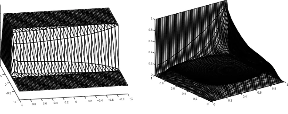
SDFEM solutions of the above problems for the case ² = 10−3are shown in Figure 4. In each problem, the linear systems are directly solved on the coarsest 4x4 grid first. Then the following procedures are followed:

−1 −0.5 0 0.5 1 −1 −0.8 −0.6 −0.4 −0.2 0 0.2 0.4 0.6 0.8 1 −0.2 0 0.2 0.4 0.6 0.8 1 1.2

(a) Solution of Problem 1 on a 32 × 32 grid

0 0.2 0.4 0.6 0.8 1 0 0.2 0.4 0.6 0.8 1 0 0.2 0.4 0.6 0.8 1

(b) Solution of Problem 2 on a 64 × 64 grid

FIG. 4.1. SDFEM solutions of Problem 1 and Problem 2 for the case ² = 10−3 1. Compute error estimator η.

2. Select elements according to the maximum marking strategy. 3. Refine selected elements and generate a new mesh.

4. Obtain the initial guess by interpolating the current solution to the new mesh. 5. Solve linear system so that a given stopping criterion Siis satisfied.

For the linear solvers, three methods, Gauss elimination (GE), the multigrid method (MG) and the generalized minimal residual method (GMRES), are used to solve linear sys-tems. In the MG solver, the prolongation operator is the standard linear interpolation, the restriction operator is the adjoint of the prolongation operator and the correction operator is obtained from direct SDFEM discretization on the coarse grid. We use the same Gauss-Seidel (GS) preconditioner for both MG and GMRES. In Problem 1, the preconditioner is one step of vertical GS sweep. In Problem 2, the preconditioner consists of one bottom-to-top vertical GS sweep, one top-to-bottom vertical GS sweep, one left-to-right horizontal GS sweep and one right-to-left horizontal GS sweep. Three different criteria Si, i = 0, 1, 2, are chosen. When S0 is given, the linear systems are solved directly by GE. When using MG and

GM-RES solvers, the stopping criterion S1represents the heuristic stopping tolerance, i.e., the L2

norm of the residual of iterative solutions less than 10−6and the stopping criteriion S2is the

criterion (3.8) in Theorem 3.2.

For the mesh refinement, the threshold θ in the maximum strategy and the number of refinement steps are carefully chosen so that more detail layer structures of the solutions can be seen during each refinement step. For both problems, the threshold is set to 0.1. For the number of refinement steps, four steps are performed for the case ² = 10−2, seven steps are performed for the case ² = 10−3, and eight steps are performed for the cases 10−4.

In the following, we compare the refined meshes generated by the error indicators com-puted from GE, MG and GMRES solutions for each problem with 3 for different values of ² = 10−2_{, 10}−3 _{and 10}−4_{. The iteration steps among different linear solvers and stopping} criteria are also compared. The error indicators computed from solutions satisfying criterion

(12)

S1,S1and S2are denoted as η0, η1and η2, respectively. Since, Table 4.1 and Table 4.4 show

that the constant αη,∞À 0 in (3.2), we set αη,∞= 0.5 in the stopping criterion S2. Table 4.2

and Table 4.5 show the number of iterations for MG and GMRES to satisfy different stopping criteria on various mesh levels. Table 4.3 and Table 4.6 show the number of nodes generated by error indicators, η0, η1and η2computed from MG solutions, along the refinement process.

From, Table 4.2 and Table 4.5, it is clear that fewer iterations are needed for MG to satisfy the criterion S2, i.e., the criterion (3.8) in Theorem 3.2. In contrast, more iterations are needed

for GMRES to satisfy S2comparing to the iterative steps needed for GMRES to satisfy S1.

The total amount of work of MG with our stopping criterion is about half of the amount of work of MG with the heuristic stopping criterion. Finally, from Table 4.3 and Table 4.6, we can see that the number of nodes of each refined mesh remains almost unchanged no matter which error indicator is used to generate the meshes.

Numerical results for Problem 1:

² maxT ∈=h ηT ηTp on refined meshes 10−2 _{0.5 0.5 0.5 0.499} 10−3 _{0.5 0.5 0.5 0.5 0.5 0.5 0.5} 10−4 _{0.5 0.5 0.5 0.5 0.5 0.5 0.5 0.5} TABLE4.1

Verification of the assumption (3.2) of the new stopping criteria

² Tol Iterations 10−2 S1 12 10 9 12 S2 4 4 4 7 10−3 S1 16 13 11 9 8 8 15 S2 7 4 4 4 3 4 13 10−4 S1 16 14 12 10 9 8 8 8 S2 9 6 5 5 4 3 3 3

(a) MG iteration steps

(b) GMRES iteration steps TABLE4.2

Comparison of iteration steps for different stopping criteria

² Error Indicator Node number

10−2 _η 0, η1, η2 50 97 190 394 10−3 η0, η1 50 91 174 343 697 1350 2702 η2 50 91 174 343 683 1359 2702 10−4 _η 0, η1 50 91 174 343 679 1346 2674 5331 η2 50 91 174 343 679 1346 2688 5334 TABLE4.3

Comparison of number of nodes of refined meshes from MG solutions

(13)

Numerical results for Problem 2: ² maxT ∈=h ηT ηTp on refined meshes 10−2 _{0.34 0.30 0.36 0.24} 10−3 _{0.34 0.37 0.51 0.68 0.75 0.44 0.17} 10−4 _{0.34 0.31 0.33 0.24 0.71 0.54 0.82 0.52} TABLE4.4

Verification of the assumption (3.2)of the new stopping criteria

(a) MG iteration steps

(b) GMRES iteration steps TABLE4.5

Comparison of iteration steps for different stopping criteria

² Error Indicator Node number

10−2 _η 0, η1, η2 70 168 390 911 10−3 η0, η1 70 176 345 592 948 1458 2391 η2 70 176 345 592 948 1458 2391 10−4 _η 0, η1 70 176 354 764 1143 1752 2674 4093 η2 70 176 354 764 1143 1750 2688 4082 TABLE4.6

Comparison of number of nodes of refined meshes from MG solutions

5. Conclusion. In this work, we have presented two stopping criteria, (3.5) and (3.8),

for the iterative linear solvers based on the a posteriori error estimations and the maximum marking strategy. We have shown that the iterative error can be bounded by the upper bound of the a posteriori error when the iterative solution satisfies the criterion (3.5). Numerical studies in [22] indicate that the a posteriori error estimations by Kay and Silvester are opti-mal. Therefore, in the sense of measuring the global true errors between numerical solutions and the weak solution of the PDE, the exact SDFEM solution and the iterative solutions sat-isfying criterion (3.5) are indistinguishable. On the other hand, although the global errors of iterative soultions can be confined by using cirterion (3.5), this criterion does not guarran-tee the effectiveness of the mesh refinement process since the marking strategy is essentially based on the local information about the error indicator. Here, we have also shown that when the error indicator is computed from iterative solutions, the criterion (3.8) can be used to avoid refinement over wrong locations or over-refinement. Numerical results in Section 4 support the effectiveness of the criterion (3.8). Moreover, we have found significant amount

(14)

of work can be saved by using the MG solver with Gauss-Seidel smoother that satisfies cri-terion (]refs3:eq18). According to this study, we suggest that the stopping cricri-terion (3.8) can be used to achieve the efficiency of the mesh refinement process and stopping criterion (3.5) should be verified at the finest mesh where a reliable solution is expected.

REFERENCES

[1] M. Ariloi. A stopping criterion for the conjugate gradient algorithm in a finite element method framework. Numer. Math., 97:1–24, 2004.

[2] M. Ariloi, I. Duff, and D. Ruiz. Stopping criteria for iterative methods. SIAM J. Matrix Anal. Appl., 13(1):138– 144, 1992.

[3] M. Ariloi, D. Loghin, and A. J. Wathen. Stopping criteria for iterations in finite element methods. RAL Technical Reports, RAL-TR-2003-009(CCLRC), 2003.

[4] M. Ariloi, E. Noulard, and A. Russo. Stopping criteria for iterative methods: applications to pde’s. CALCOLO, 38:97–112, 2001.

[5] L. Reichel D. Calvetti, S. Morigi and F. Sgallari. An iterative method with error estimators. J. Comp. Appl. Math., 127:93–119, 2001.

[6] W. D¨orfler and R. H. Nochetto. Small data oscillation implies the saturation assumption. Numer. Math., 91:1–12, 2002.

[7] K. Eriksson and C. Johnson. Adaptive streamline diffusion finite element methods for stationary convection-diffusion problems. Math. Comp., 60:167–188, 1993.

[8] B. Fischer, A. Ramage, D. Silvester, and A. J. Wathen. On parameter choice and iterative convergence for stabilised discretisations of advection-diffusion problems. Comput. Methods Appl. Mech. Engrg., 179, 1999.

[9] G. H. Golub and G. Meurant. Matrices, moments and quadrature, volume 303 of Numerical Analysis (1993), D. F. Griffiths and G. A. Watson (Eds),. Pitman Research Notes in Mathematics, 1994.

[10] G. H. Golub and G. Meurant. Matrices, moments and quadrature II: how to compute the norm of the error in iterative methods. BIT, 37:687–705, 1997.

[11] G. H. Golub and Z. Strakoˇs. Estimated in quadratic formulas. Numer. Algorithms., 8:241–268, 1994. [12] T. Hughes and A. Brooks. A multidimensional upwind scheme with no crosswind diffusion. Finite Element

Methods for Convection Dominated Folws, AMSE, New York, 34, 1979.

[13] T. J. R. Hughes, M Mallet, and A. Mizukami. A new finite element formulation for computational fluid dynamics: II. Beyond SUPG. Comput. Methods Appl. Mech. Engrg., 54:485–501, 1986.

[14] D. Kay and D. Silvester. The reliability of local error estimators for convection-diffusion equations. IMA. Journal of Num. Anal., 21:107–122, 2001.

[15] K. Mekchay and R. H. Nochetto. Convergence of adaptive finite element methods for general second order linear elliptic pde. preprint.

[16] G. Meurant. The computation of bounds for the norm of the error in the conjugate gradient algorithm. Numer. Algorithms, 16:77–87, 1997.

[17] K. Niijima. Pointwise error estimates for a streamline diffusion finite element scheme. Numer. Math., 56:707– 719, 1990.

[18] A. Papastavrou and R. Verf¨urth. A posteriori error estimators for stationary convection-diffusion problems: a computational comparison. Comput. Methods Appl. Mech. Engrg., 189:449–462, 2000.

[19] M. C. Rivara. Algorithms for refining triangular grids suitable for adaptive and multigrid techniques. Int. J. Numer. Methods Eng., 20:745–756, 1984.

[20] M. C. Rivara. Using longest-side bisection techniques for the automatic refinement of Delaunay triangulation. Int. J. Numer. Methods Eng., 40:581–597, 1997.

[21] R. Verf¨urth. A posteriori error estimators for convection-diffusion equations. Numer. Math., 80:641–663, 1998.

[22] Chin-Tien Wu. On the implementation of an accurate and efficient solver for convection-diffusion equations. PhD thesis, University of Maryland at College Park, 2003.