於雙眼建築場景中保留透視圖法及視差特性的影像修補方法

國

立

交

通

大

學

多媒體工程研究所

碩

士

論

文

於雙眼建築場景中保留透視圖法及視差特性的影像修補方法

Perspective and Parallax Preserved Inpainting for Stereoscopic Architectural

Scene Images

研 究 生：陸品樺

指導教授：林奕成 教授

於雙眼建築場景中保留透視圖法及視差特性的影像修補方法

Perspective and Parallax Preserved Inpainting for Stereoscopic Architectural

Scene Images

研 究 生：陸品樺 Student：Pin-Hua Lu

指導教授：林奕成 Advisor：I-Chen Lin

國 立 交 通 大 學

多 媒 體 工 程 研 究 所

碩 士 論 文

Submitted to Institute of Multimedia Engineering College of Computer Science

National Chiao Tung University in partial Fulfillment of the Requirements

for the Degree of Master

in

Computer Science

September 2011

Hsinchu, Taiwan, Republic of China

I

於雙眼建築場景中保留透視圖法及視差特性的影像修補方法

研究生: 陸品樺 指導教授: 林奕成 教授

國立交通大學

多媒體工程研究所

摘要

II

Perspective and Parallax Preserved Inpainting for Stereoscopic

Architectural Scene Images

Student: Pin-Hua Lu Advisor: Prof. I-Chen Lin

Institute of Multimedia Engineering

National Chiao Tung University

ABSTRACT

Image completion algorithms are powerful for removing undesirable obstacle objects. Nevertheless, when the undesirable obstacle objects cover a large amount of the background and the background is artificial constructed, structure of the background is difficult to maintain. In this thesis, we present an automatic image completion method for stereoscopic architectural scene images. We take advantage of two-view information to reduce obstacle pixels and preserve parallax consistency. A vanishing point and vanishing line prediction is used to perspective correct the input images to eliminate perspective artifacts. A structure-enhanced patch searching algorithm is also proposed to preserve the architectural structure. The proposed method is performed on a number of artificial construction images to show reasonable results.

III

Acknowledgement

IV

Content

Chapter 2 Related Work...3

Chapter 3 Overview...6

Chapter 4 Preprocessing of Disparity Maps and Images...10

4.1 Occlusion Filling for Disparity Map...10

4.2 Image Completion through Warping from another Viewpoint...13

Chapter 5 Automatic Perspective Correction...17

5.1 Vanishing Point Predicting...17

5.2 Perspective Correction...20

Chapter 6 Image Completion Through Exemplar-Based Inpainting...23

6.1 Exemplar-Based Inpainting...24

6.1.1 Determining the filling order...24

6.1.2 Finding the source patch...25

6.2 Consistency Check...28

Chapter 7 Results and Discussion...30

7.1 Results...31

7.2 Discussion...59

Chapter 8 Conclusions...60

V

List of Figure

Figure 1: Symbol definition...8

Figure 2: System flow chart...9

Figure 3: Handling the occlusion parts of the disparity maps. Red area is occlusion parts and grey area is known disparity values. Black slash area is one of the segments. Left, middle and right picture shows the segment of 𝑆̃𝑁𝑜𝑛_𝑂𝑐𝑐 , 𝑆̃_{𝑃𝑎𝑟𝑡_𝑂𝑐𝑐} and 𝑆̃𝑂𝑐𝑐 ...11

Figure 4: One view of the stereo image inputs...15

Figure 5: Red area is user defined foreground object...15

Figure 6: After warping from another view...16

Figure 7: Each point on a structure line use a single Gaussian to vote for the position of vanishing point...19

Figure 8: 5x5 discrete Gaussian kernel...20

Figure 9: Vanishing lines and vanishing point prediction. Purple lines are vanishing lines, and green spot is the predicted vanishing point. The yellow spots and blue lines obtain the grid aligned the building plane...21

Figure 10: Perspective corrective space...22

Figure 11: Structure-enhanced patch searching algorithm...27

Figure 12: Input stereo images and user defined obstacle pixels (red pixels)...31

Figure 13: Four iterations of original stereoscopic inpainting. Top to bottom: iteration 1 to 4...32

Figure 14: Fourth iteration of one view in Figure 13...33

Figure 15: Four iterations of our method without structure enhancement. Top to bottom: iteration 1 to 4...34

Figure 16: Fourth iteration of one view in Figure 15...35

Figure 17: Four iterations of our method with structure enhancement. Top to bottom: iteration 1 to 4...36

VI

Figure 18: Fourth iteration of one view in Figure 17...37 Figure 19: Comparison of three approaches. Left to right: Original stereoscopic

inpainting, our method without structure enhancement, our method with structure enhancement...37 Figure 20: Input stereo images and user defined obstacle pixels (red pixels)...38 Figure 21: Four iterations of original stereoscopic inpainting. Top to bottom: iteration

1 to 4...39 Figure 22: Fourth iteration of one view in Figure 21...40 Figure 23: Four iterations of our method without structure enhancement. Top to

bottom: iteration 1 to 4...41 Figure 24: Fourth iteration of one view in Figure 23...42 Figure 25: Four iterations of our method with structure enhancement. Top to bottom:

iteration 1 to 4...43 Figure 26: Fourth iteration of one view in Figure 25...44 Figure 27: Comparison of three approaches. Left to right: Original stereoscopic

inpainting, our method without structure enhancement, our method with structure enhancement...44 Figure 28: Input stereo images and user defined obstacle pixels (red pixels)...45 Figure 29: Four iterations of original stereoscopic inpainting. Top to bottom: iteration

1 to 4...46 Figure 30: Fourth iteration of one view in Figure 29...47 Figure 31: Four iterations of our method without structure enhancement. Top to

bottom: iteration 1 to 4...48 Figure 32: Fourth iteration of one view in Figure 31...49 Figure 33: Four iterations of our method with structure enhancement. Top to bottom:

iteration 1 to 4...50 Figure 34: Fourth iteration of one view in Figure 33...51 Figure 35: Comparison of three approaches . Left to right: Original stereoscopic

VII

structure enhancement...51 Figure 36: Input stereo images and user defined obstacle pixels (red pixels)...52 Figure 37: Four iterations of original stereoscopic inpainting. Top to bottom: iteration

1 to 4...53 Figure 38: Fourth iteration of one view in Figure 37...54 Figure 39: Four iterations of our method without structure enhancement. Top to

bottom: iteration 1 to 4...55 Figure 40: Fourth iteration of one view in Figure 39...56 Figure 41: Four iterations of our method with structure enhancement. Top to bottom:

iteration 1 to 4...57 Figure 42: Fourth iteration of one view in Figure 41...58 Figure 43: Comparison of three approaches. Left to right: Original stereoscopic

inpainting, our method without structure enhancement, our method with structure enhancement...58

1

Chapter 1

Introduction

Digital cameras have become prevalent for daily use. People use digital photos to record landscapes and landmarks during their trips. But the picture is rarely “perfect” due to the complex surrounding and framing preference. Obstacles like trees, street lights or commercial flags often play a role as undesirable objects covering the main character of the scene.

In this thesis, we focus on the photos in an architecture theme. The main subject of the photo is buildings or artificialities with structural design like brick walls. Users specified obstacle object that need to be removed. The foreground object removal remains a hole in the image and needed to be filled. It results in an image completion problem.

Example-base image inpainting, a digital image processing technique is widely used to fill in the holes caused by removing foreground objects in an image. But strong artifacts may appear during the inpainting process and make the synthesized region incompatible with the real part.

Wang et al. proposed a stereoscopic inpainting algorithm [WAN08], using stereo images with corresponding disparity maps. The algorithm improves the traditional

2

example-based single image inpainting. It takes advantage of the two-view and disparity information to produce a more reasonable result.

The conceptual idea of example-based inpainting is to fill missing pixels by copying small fragments from known region. It assumes the fragments are aligned with the image plane. Nevertheless, this is barely satisfied in architecture-themed photos unless the photo is taken in the frontal view. The perspective artifacts heavily influence the image completion result.

The oblique fragment problem can be solved through orientation indication by skilled users. However, in an architecture-themed photos limitation, there are some special characteristics in buildings that can help performing automatically perspective correction process.

We propose a system for removing foreground objects in stereo architecture-themed photos with automatic perspective correction. The system uses an automatic vanishing point prediction to estimate the main building orientation and performs perspective correction. With perspective correction, perspective artifacts that may not be detected during the consistency-check can be alleviated. We also applied a structure-enhanced patch searching method to better connect the structure lines. In addition to the automatic perspective correction, our approach takes advantage of the strength of stereoscopic inpainting for more reasonable image completion.

3

Chapter 2

Related Work

Our work is related to the literature of image completion. Image completion algorithms deal with the problem of filling missing region in images. Two fundamental approaches have been proposed to solve the image completion problem: image inpainting methods and example-based approaches.

Image inpainting methods are good at filling narrow gaps like speckles, scratches, and overlaid text in image [BCV01;BBS01;BSC00;CHA01;MAS98]. Image inpainting considers that images are composed by structures, shapes, and objects separating from one another by sharp edges. The term “digital image inpainting” was first introduced in [BSC00] by Bertalmio et al. These inpainting techniques propagate linear structures, called isophotes, to fill the gaps in image. They were inspired by partial differential equations (PDEs), and worked as restoration algorithms. When dealing with larger missing regions, noticeable blurring effect may occur during the diffusion process.

Example-based approaches took advantage of texture synthesis to avoid blurring effect, where large texture patches are synthesized from small texture samples. Bertalmio et al. pioneered at this approach [BVS03]. Their algorithm decomposes image into image structure and texture components. The image structure part is then processed by inpainting

4

method, and the texture part is processed by texture synthesis on per-pixel basis. Two components are summed to be the result image. However, working on per-pixel basis still remains limited to removing small missing gaps. Fragment-based approaches [BAR02; CPT03; DCY03] usually produce better results on larger missing areas. Drori et al. proposed an algorithm [DCY03] to iteratively find and copy similar circular image fragment to current unknown location. The results of [DCY03] were impressive but time consuming. Criminisi et al. proposed a patch-based greedy sampling algorithm [CPT03] like fragment-based approach, but faster and simpler. They determined filling orders at missing region boundary with a priority measurement different from original onion peeling algorithm. The priority is obtained by measuring the surrounding known pixels and isophote strength.

Some completion approaches from multiple images have been explored in the last decade. Chan et al. use an additional image as reference [CHA02]. They applied landmark matching to calculate an affine mapping between reference image and the input image. And the warped patches were copied to recover the missing part of the input image. Wilczkowial

et al. [WBT05] and Hays et al. [HAY07] used multiple images to increase the sampling

space. While the same scene but different view images are used in [WBT05], large amount of different scene images are used in [HAY07]. Bhat et al. [BHA07] used depth information estimated from a video sequence to guild the sampling process. However, this work requires a large number of nearby video frames. Wang et al. proposed a stereoscopic inpainting algorithm [WAN08] which takes a pair of stereo images and disparity maps as input. In the work of Wang et al. [WAN08], disparity maps could be precalculated by any existing stereo algorithm and help the inpainting process.

5

information to help the completion process. Sun et al. [SYJ05] proposed an interactive completion approach that users provided feature curves and image structure propagation. Pavić et al. presented a system [PSK06] which allowed users to define 3D planes by marking quads on input image for perspective correction. They relieved the fragment alignment problem in fragment-based approaches.

In addition to image completion, our work uses an automatic perspective correction based on vanishing point and vanishing line geometry and is related to vanishing point prediction. Many vanishing point prediction algorithm have been proposed. Gaussian Sphere approach was first present by Barnard [BAR83]. This approach transfers line segments in the image to circles on the Gaussian sphere and a point on the Gaussian sphere corresponds to a vanishing point in the image. Some methods have been proposed to enhance Gaussian Sphere approach. Almansa et al. [ADV03] proposed a method that combined Gaussian sphere and Hough transform. And Aguilera et al. [ALC05] suggest a combination of RANSAC and Gaussian Sphere method to detect both vanishing points and vanishing directions. Coughlan et al. [CY99; CY03] determined the orientation of the viewer in the scene using Bayesian Model under the Manhattan assumptions, which is satisfied in most indoor and outdoor city scenes. This manner was then extended by [SD04] with expectation maximization (EM) method to estimate the vanishing directions.

6

Chapter 3

Overview

Our method is mainly inspired by the Stereoscopic Inpaint algorithm, presented by Wang et al. [WAN08] They use a warping algorithm to first fill the missing pixels from the two view information introduced by stereo images. And they used a refined exemplar-based inpaint [CPT03] to complete the rest missing pixels. They also proposed a method to check the filling pixels’ consistency and detect unreliable pixels.

We use the framework of Stereoscopic Inpainting to decrease obstacle pixels and check the consistency of inpainting results. Furthermore, we propose an automatic vanishing point and vanishing lines prediction for perspective correction. The exemplar-based inpainting algorithm is then performed on the perspective corrected space. And we further modify the patch searching algorithm in exemplar-based inpainting to preserve the vanishing line structure of the building.

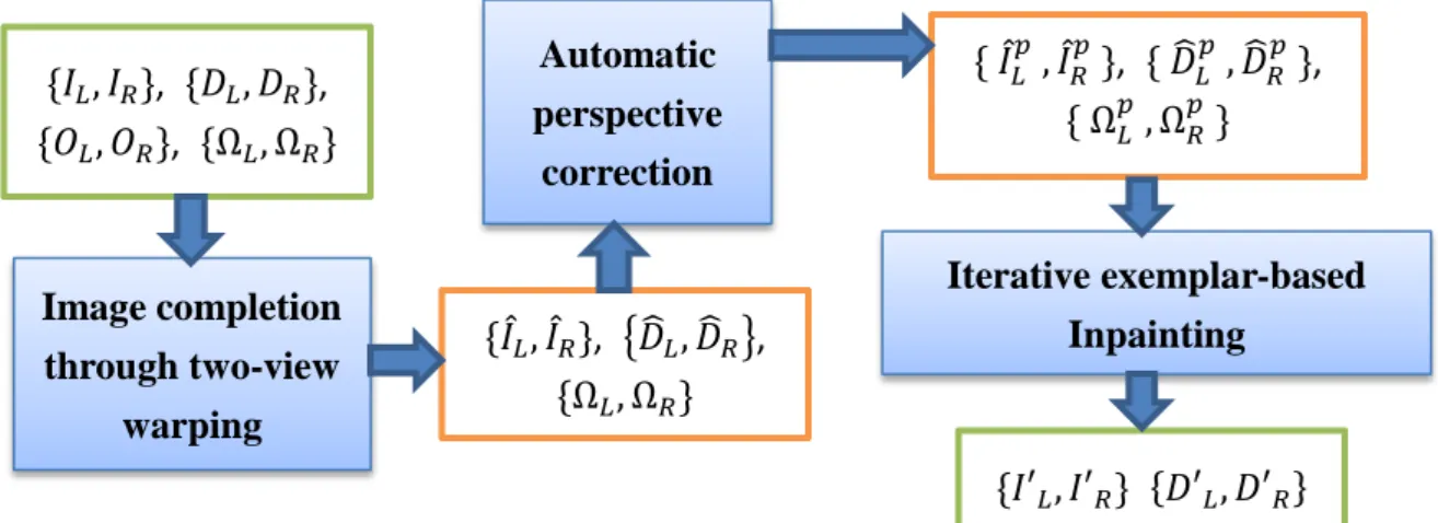
There are three main stages in our inpainting system:

1. Image completion through two-view warping:

To execute the warping stage, we need to first fill the occluded pixels in the disparity maps. A segmentation-based approach is used to accomplish the disparity maps. Missing pixels are mostly covered by the removed foreground object. These missing pixels may be visible

7

in the other view and can be filled by warping from the other image.

2. Automatic perspective correction:

After the warping stage, there are still missing pixels in stereo images that cannot be seen in both views. We use an exemplar-based inpainting algorithm performed on perspective corrected space to fill them. An automatic perspective correction mapping matrix is calculated by estimating the vanishing point and vanishing lines of the main building in the images.

3. Iterative Exemplar-based Inpainting:

A modified exemplar-based inpainting is proposeed to complete the stereo images and the disparity maps. By checking the color consistency of the filled pixels utilizing the characteristic of stereo images, we can detect the unreliable filling results. Re-inpainting these unreliable pixels forms an iterative inpainting scheme, and produces a more reasonable completion.

We take stereo images *𝐼_𝐿, 𝐼_𝑅+, disparity maps *𝐷_𝐿, 𝐷_𝑅+, and sets of occluded pixels in the two views *𝑂_𝐿, 𝑂_𝑅+ as input. User defines the removing foreground object pixels as *Ω_𝐿, Ω_𝑅+. The first stage fills the occluded pixels in disparity maps, and the result is denoted as *𝐷̅𝐿, 𝐷̅𝑅+. For the pixels in Ω𝐿 that are visible in the right view and the pixels in Ω𝑅

that are visible in the left view, we warp 𝐼_𝐿 using 𝐷̅_𝐿 to the right view and 𝐼_𝑅 using 𝐷̅_𝑅 to the left view. The warping result is denoted as {𝐷̂𝐿, 𝐷̂𝑅} and *𝐼̂𝐿, 𝐼̂𝑅+. In the second stage,

the result of perspective corrected images and disparity maps are denoted as * 𝐼̂_𝐿𝑝 , 𝐼̂_𝑅𝑝 + and * 𝐷̂_𝐿𝑝 , 𝐷̂_𝑅𝑝 +. The third stage completes both color and disparity values, referred as *𝐼′𝐿, 𝐼′𝑅+

8

Figure 1: Symbol defination

Image completion through two-view warping Automatic perspective correction Iterative exemplar-based Inpainting *𝐼_𝐿, 𝐼_𝑅+, *𝐷𝐿, 𝐷𝑅+, *𝑂_𝐿, 𝑂_𝑅+, *Ω𝐿, Ω𝑅+ *Ω𝐿, Ω𝑅+ *𝐼̂_𝐿, 𝐼̂_𝑅+, {𝐷̂𝐿, 𝐷̂𝑅}, * Ω_𝐿𝑝 , Ω_𝑅𝑝 + * 𝐼̂_𝐿𝑝 , 𝐼̂_𝑅𝑝 +, * 𝐷̂_𝐿𝑝 , 𝐷̂_𝑅𝑝 +, *𝐼′_𝐿, 𝐼′_𝑅+ *𝐷′𝐿, 𝐷′𝑅+

9

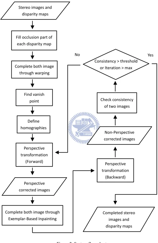
Figure 2: System flow chart. Stereo images and

disparity maps

Find vanish point

Complete both image through warping Fill occlusion part of

each disparity map

Define homographies Perspective transformation (Forward) _Perspective transformation (Backward)

Complete both image through Exemplar-Based Inpainting Check consistency of two images Perspective corrected images Non-Perspective corrected images Consistency > threshold or Iteration > max Completed stereo images and disparity maps Yes No

10

Chapter 4

Preprocessing of Disparity Maps and Images

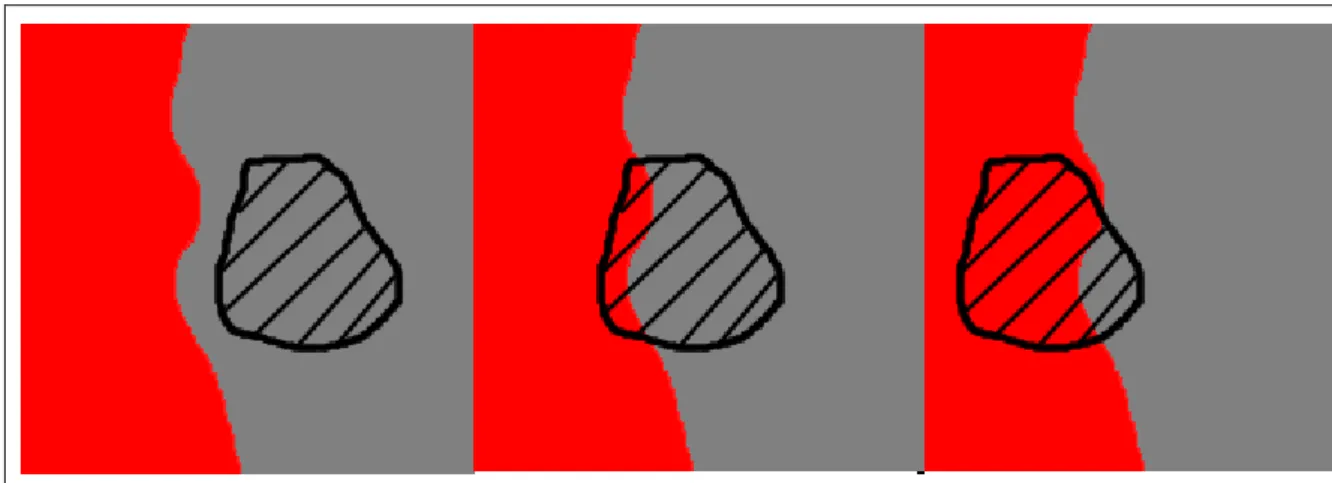
4.1 Occlusion Filling for Disparity Map

The occlusion filling process for the two input disparity maps are performed independently. Taking disparity maps * 𝐷_𝐿 , 𝐷_𝑅 + and sets of occluded pixels * 𝑂_𝐿 , 𝑂_𝑅 + as input, * 𝐷̅𝐿 , 𝐷̅𝑅 + denote the left and right disparity maps after occlusion filling. Since the

process for two disparity maps have the same scheme, we will only describe the process for one view in detail.

By the widely used segment constraint, the disparity values of a small segment region change very smoothly. A 3D plane can be used to model the disparity values in a region. First the input images are split into small regions. We perform the mean shift segmentation

[COM02]on the input stereo images for clustering. Adjacent pixels with similar colors are

grouped into a set of segments 𝑆̃ = * 𝑆₁ , 𝑆₂ , … +. Note that a larger segment region leads to a smoother result, but a smaller segment region better satisfies the segment constraint.

With the occlusion maps * 𝑂_𝐿 , 𝑂_𝑅 +, we further classify the segments into three sets to fill disparity values for pixels in 𝑂 ⊂ 𝑂_𝐿:

11

𝑆̃_{𝑁𝑜𝑛_𝑂𝑐𝑐} = * 𝑆|𝑆 ∈ 𝑆̃ ∧ ||𝑆 ∩ 𝑂|| = 0 + (1) 𝑆̃_{𝑃𝑎𝑟𝑡_𝑂𝑐𝑐} = * 𝑆|𝑆 ∈ 𝑆̃ ∧ ||𝑆 ∩ 𝑂|| > 0 ∧ ||𝑆 − 𝑂|| > 𝜆 ∙ ||𝑆|| + (2) 𝑆̃_𝑂𝑐𝑐 = * 𝑆|𝑆 ∈ 𝑆̃ ∧ ||𝑆 ∩ 𝑂|| > 0 ∧ ||𝑆 − 𝑂|| < 𝜆 ∙ ||𝑆|| + (3)

The elements in 𝑆̃_{𝑁𝑜𝑛_𝑂𝑐𝑐} , 𝑆̃_{𝑃𝑎𝑟𝑡_𝑂𝑐𝑐} and 𝑆̃_𝑂𝑐𝑐 stand for segment regions which have different ratio of overlapping pixels with the occluded pixels.

For segment regions in 𝑆̃_{𝑁𝑜𝑛_𝑂𝑐𝑐} , all disparity values are known and can be modeled

by a set of 3D plane parameters, therefore, we apply a RANSAC[FIS81] based plane fitting

algorithm to assign disparity planes to these segment regions.

For segment regions in 𝑆̃_{𝑃𝑎𝑟𝑡_𝑂𝑐𝑐} and 𝑆̃_𝑂𝑐𝑐 , there are missing disparity values.

Consider a segment region S, disparity value 𝑑𝑖𝑠𝑝 ∈ 𝑆 ∩ 𝑂 is unknown, and our goal is to

assign a disparity plane to S, so that disp can be calculated through the plane parameters. Figure 3: Handling the occlusion parts of the disparity maps. Red area is occlusion parts and grey area is known disparity values. Black slash area is one of the segments. Left, middle and right picture shows the segment of 𝑆̃𝑁𝑜𝑛_𝑂𝑐𝑐 , 𝑆̃𝑃𝑎𝑟𝑡_𝑂𝑐𝑐 and 𝑆̃𝑂𝑐𝑐 .

12

Segment regions in 𝑆̃_{𝑃𝑎𝑟𝑡_𝑂𝑐𝑐} and 𝑆̃_𝑂𝑐𝑐 have different ratio of known disparity values, and λ is the measurement threshold. Depending on the ratio of known pixels, two different filling approaches are used.

Segment regions in 𝑆̃_{𝑃𝑎𝑟𝑡_𝑂𝑐𝑐} are considered have sufficient known pixels to determine a representational disparity plane. Therefore the plane parameters can be computed based on pixels in set S – O using RANSAC plane fitting algorithm, and then the occluded pixels are calculated through the plane parameters.

For 𝑆̃_𝑂𝑐𝑐 , due to the lack of known disparity values in segment regions, we need to find optimal disparity planes for the segments. A greedy algorithm is used to assign proper plane parameters. Searching for the segment pair（t, s）that minimizes a matching cost E(t, s), where t is the target segment with no plane parameter assigned yet and s is the source segment already having a set of plane parameters. Once segment pair（t, s）is found, plane parameters of s is assigned to t, and the unknown disparity values can be filled. The matching cost E(t, s) is defined as a weighted sum of three terms:

𝐸(𝑡, 𝑠) = 𝐸_𝑐𝑙𝑟(𝑡, 𝑠) + 𝜆_𝑎𝑑𝑗𝐸_𝑎𝑑𝑗(𝑡, 𝑠) + 𝜆_𝑣𝑖𝑠𝐸_𝑣𝑖𝑠(𝑡, 𝑠) (4) Where 𝐸_𝑐𝑙𝑟(𝑡, 𝑠) is the measurement for color similarity between two segments. It is defined as:

𝐸_𝑐𝑙𝑟(𝑡, 𝑠) = 1 − 𝐶⃑𝑡∙𝐶⃑𝑠

‖𝐶⃑𝑡‖∙‖𝐶⃑𝑠‖ (5)

𝐶⃑_𝑡 and 𝐶⃑_𝑠 are the average color vectors of segments t and s. 𝐸_𝑎𝑑𝑗 is a binary adjacency function used to determine whether t and s are adjacent. It returns 1 if the two segments are neighbors. This term is added due to that neighboring segments tend to have similar plane

13

parameters. 𝐸_𝑣𝑖𝑠(𝑡, 𝑠) penalizes disparity assignments that cause inconsistent visibility relationships. The weak consistency constraint [GON03] pointed out that occluded pixels must be occluded by a closer object, which means occluded pixels must have smaller disparity value than its corresponding pixel in the other disparity map:

𝐷̅_𝐿(𝑥, 𝑦) ≤ 𝐷̅_𝑅(𝑥 − 𝐷̅_𝐿(𝑥, 𝑦), 𝑦) (6) 𝐷̅𝑅(𝑥, 𝑦) ≤ 𝐷̅𝐿(𝑥 + 𝐷̅𝑅(𝑥, 𝑦), 𝑦) (7)

𝐸_𝑣𝑖𝑠(𝑡, 𝑠) returns the ratio of pixels in t that violate this constraint.

4.2 Image Completion through Warping from another Viewpoint

User Specifies pixels of foreground objects to be removed as * Ω_𝐿 , Ω_𝑅 +. Removing these pixels will leave holes in input images and disparity maps. Thanks to the image from another view, we have additional information to complete the image. Our goal in this stage is to fill these pixels through warping from the other view. The results are images *𝐼̂_𝐿, 𝐼̂_𝑅+ and disparity maps *𝐷̂_𝐿, 𝐷̂_𝑅+.

Stereo images with disparity maps can consider as two images with per-pixel correspondence. In the prior section, we recovered the disparity values of occluded parts. Which means the corresponding positions of the occluded pixels in each other image is known. After removing foreground objects in one view, part of the background objects which are not covered by foreground objects in another view can be seen. Hence, we can mutually complete each other image through 3D warping [MMB97]. For the right view completion, if(𝑥 − 𝐷̅_𝐿(x, y), y) ∈ Ω_𝑅, we can set:

14

𝐼̂𝑅(𝑥 − 𝐷̅𝐿(𝑥, 𝑦), 𝑦) = 𝐼𝐿(𝑥, 𝑦)

𝐷̂_𝑅(𝑥 − 𝐷̅_𝐿(𝑥, 𝑦), 𝑦) = 𝐷_𝐿(𝑥, 𝑦) (8) Similarly, for the left view completion, if(𝑥 + 𝐷̅_𝑅(x, y), y) ∈ Ω𝐿, we can set:

𝐼̂𝐿(𝑥 + 𝐷̅𝑅(𝑥, 𝑦), 𝑦) = 𝐼𝑅(𝑥, 𝑦)

𝐷̂_𝐿(𝑥 + 𝐷̅_𝑅(𝑥, 𝑦), 𝑦) = 𝐷_𝑅(𝑥, 𝑦) (9) During the warping process, when multiple pixels are warped to a same destination, we choose the one with the largest disparity value because smaller disparity value means a larger distance from the viewpoint and should not be visible.

Pixels satisfy above conditions are filled with color and disparity values through warping and are removed from * Ω_𝐿 , Ω_𝑅 +. This reduces the amount of pixels to be filled, and because the warped pixels are real “seen” in the other view, the filling result is more natural and reasonable.

15

Figure 4: One view of the stereo image inputs.

16

17

Chapter 5

Automatic Perspective Correction

Fragment-based image completion techniques are powerful tools and often used to fill in missing pixel information caused by foreground object removal. The conceptual idea is to repeatedly fill missing pixels by copying small source fragment from known regions of the image and eventually complete the whole missing region. The fundamental assumption of fragment-based image completion approaches is that for a small enough fragment, it is considered to be nearly planar. However, fragment planes may not aligned to the view plane in real world photos. Simply copying pixels from source fragment may cause perspective artifacts.

In [DVL06], authors presented an interactive system for exploiting information about

the approximate 3D structure in a scene in order to estimate and apply perspective corrections. The system requires user to sketch convex quad-grids to calculate a 3 x 3 homography matrix which rectifies the grids aligned to the view plane. In this chapter, we propose a scheme which can automatically define a proper convex grid for perspective correction using the vanish lines in single image. The process is applied independently to both stereo images.

18

3D parallel lines under perspective projection meet a point in an image called vanishing point, and the lines intersecting at vanishing point are called vanishing lines. For artificialities, structure lines of a plane tend to be aligned to each other in parallel or orthogonal. This phenomenon is most satisfied in architecture designs. Therefore, for an architectural scene with a single horizontal vanishing point, the vanishing point should be an assembly point of a large proportion of lines in the image. We propose learning a model

P( x | I ) to predict the position x of the vanishing point in the image. We also assume that

from salient lines are of high potential to be vanishing lines in the image.

Our goal is to find strong structure lines in the image, and the rendezvous of these lines are the potential vanishing points. First we use canny edge detection [CAN86] to provide strong edge information in the image. A strong structure line can be considered as a line on which lies many edge pixels. Here, we use Hough Transform [DOH72] to detect the strong structure lines. In the image space, a straight line can be described as:

𝑦 = − .𝑐𝑜𝑠 _𝑠𝑖𝑛 / 𝑥 + (_𝑠𝑖𝑛 ) (10) The parameter γ stands for the distance between the line and the origin, while θ is the angle of the vector from the origin to this closest point. Therefore a straight line can be represented as a point (γ, θ) in the parameter space. However, a point in image space is represented as a sinusoidal curve in the (γ, θ) plane. The idea of Hough Transform for detecting straight lines is to draw sinusoidal curves on the (γ, θ) plane for each edge pixel’s coordinate in image plane. For position p with (γp, θp) in the parameter space with sufficient

curves passing through, it indicates that the line parameter γp and θp may contain a strong

19

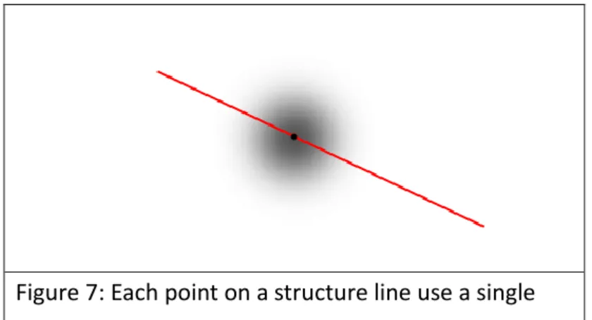
We obtain a strong structure line set 𝐿 = * 𝑙₁ , 𝑙₂ , … + . Each structure line subsequently casts probabilistic votes for possible vanishing point positions, where the hypothesis score is obtained as a sum over all votes. The score function S is defined as a probability density over the vanishing point position x = (x, y) in the image I:

(x|𝐼) ∑_𝑙∈𝐿 (x|𝑙) (𝑙|𝐼) (11) The functions P( l | I ) specifies strong structure line l found in the image I, which then votes for the vanishing point position x by P( x | l ). By analyzing this voting space, vanishing point can be predicted.

Figure 7: Each point on a structure line use a single Gaussian to vote for the position of vanishing point.

Each structure line 𝑙 ∈ 𝐿 in the image is a potential vanishing line and votes for the vanishing point. Practically, we maintain an two dimension accumulator Iacc to record the

voting score. A 5x5 discrete Gaussian kernel is applied on every pixel that structure line l passing through on the accumulator space.

20 1 4 7 4 1 4 16 26 16 4 7 26 41 26 7 4 16 26 16 4 1 4 7 4 1

Figure 8: 5x5 discrete Gaussian kernel.

Note that Iacc has a greater size than image I since the vanishing point may be out of the

image.

We further suppress wrong vanishing point prediction by choosing Mth highest scored vanishing point candidates ̅ = * ₁… + from Iacc, and then check for the amount of

corresponding vanishing lines. Structure line 𝑙 ∈ 𝐿 is considered a corresponding

vanishing line of a vanishing point candidate _𝑚 ∈ ̅ if the distance between Vm and l is

less than a threshold σ. The candidate with most vanishing lines is marked as the vanishing point of the image, and the vanishing lines corresponding to the vanishing point is marked as the vanishing lines of the image. Thus we obtained vanishing points {VL , VR} and

horizontal vanishing line sets {VLL, VLR} for the stereo images.

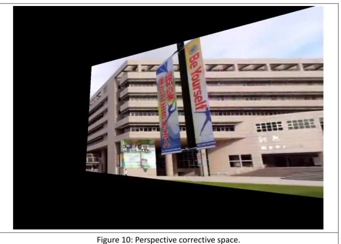
5.2 Perspective Correction

We want to define a 3x3 homographic transform A to map (X, Y), the coordinate of source image to (x, y), the coordinate of target image in which the building plane is aligned to the view plane:

21 [ 𝑤𝑥 𝑤𝑦 𝑤] = 𝐴 [ 𝑋 𝑌 1 ] (12)

A simple way is to provide two convex grids with endpoints correspondence, aligned the building plane and to the view plane. Here, we use two horizontal vanishing lines and two vertical lines that lie on the building plane to stretch the first grid. While {VLL, VLR}

provide the two horizontal vanishing lines, two vertical lines are chosen from the structure lines that are not marked as vanishing lines. Since structure lines at the linked edge of two walls are nearly perpendicular to the ground plane and the photo’s optical axis is usually parallel to the ground plane, structure lines with small orientation difference from the y-axis in the image space can be used as vertical lines. Since the mapping matrix is applied to all pixels in the source image, the size of the grids are not so important. We can pick any two horizontal vanishing lines and two vertical lines to form the grid aligned to the building plane. The grid aligned to the view plane is defined as a rectangular that is just enough to contain the first grid. In this manner, the correspondence of the endpoints is acquired intuitively.

Figure 9: Vanishing lines and vanishing point prediction. Purple lines are vanishing lines, and green spot is the predicted vanishing point. The yellow spots and blue lines obtain the

22

Note that the vertical lines in an image may not be so strong because of the obstacle in front of the building or bad framing. We can use the found vertical lines from the other view since the move of the camera between stereo images is horizontal. If there are no appropriate vertical lines in both images, y-axis can be used to derive an acceptable result. After the grids are defined, A can be computed using least square method. The perspective corrected images * 𝐼̂_𝐿𝑝 , 𝐼̂_𝑅𝑝 + and their correspond disparity maps * 𝐷̂_𝐿𝑝 , 𝐷̂_𝑅𝑝 + are obtained by applying A to * 𝐼̂_𝐿 , 𝐼̂_𝑅 + and * 𝐷̂_𝐿 , 𝐷̂_𝑅 +.

23

Chapter 6

Image Completion Through Exemplar-Based

Inpainting

In warping stage, the pixels, covered by the foreground object and visible in the other view, are already filled and removed from * Ω_𝐿 , Ω_𝑅 +. The rest pixels in * Ω_𝐿 , Ω_𝑅 + are invisible in both stereo images. Here, we extend an exemplar-based inpaintint algorithm [CPT03] to fill these pixels in each image independently. Since we have additional disparity maps, the energy function used to find optimal patch in [CPT03] can be improved for a more reasonable result as mentioned in [WAN08].

In chapter five, we use an automatic perspective correction scheme to further reduce the perspective artifacts caused by the patches which are not aligned to the image plane. After the perspective correction step, we obtained perspective corrected images * 𝐼̂_𝐿𝑝 , 𝐼̂_𝑅𝑝 + with corresponding disparity maps * 𝐷̂_𝐿𝑝 , 𝐷̂_𝑅𝑝 +, the removed foreground object regions to be filled are * Ω_𝐿𝑝 , Ω_𝑅𝑝 +. The inpainting step is performed on the perspective corrected space.

With per pixel correspondence through stereo images and disparity maps, we can cross verify the consistence of the two completed images for unreasonable results and re-inpaint the inappropriate pixels.

24

6.1 Exemplar-Based Inpainting

In the work of Criminisi et al. [CPT03], authors proposed an efficient algorithm that combines the advantages of “texture synthesis” and “inpainting” They determined the optimal order in filling unknown pixels and used an exemplar-based texture synthesis for propagating linear image structures.

We use Ψp to denote a square patch, of size m*m pixels, centered at pixel p, Φ as the

source region that provides samples, and Ω as the region need to be filled. The whole process can be split into a two-step iterative algorithm. First, we find the contour δΩ of the target region Ω and calculate the priority value of each patch Ψ = { Ψ_𝑝| 𝑝 ∈ 𝛿Ω }. The one with the highest priority value will be filled first. Once the target patch Ψt is determined, we

search for a source patch Ψs to fill the unknown pixels in Ψt. The process continues until

there are no pixels in Ω.

6.1.1 Determining the filling order

At the begining of each iteration, we decide the target patch Ψt that should be

filled first. Given a patch Ψp centered at the point p for some 𝑝 ∈ δΩ, we calculate a

priority value P(p) to decide the filling order. The concept of priority is to find patches that are on the continuation of strong edges and surrounded by reliable pixels. Filling these patches first preserves the structure of the image and leads to a reasonable result.

The priority P(p) is computed as:

25

where C(p) is the confidence term to measure the surrounded pixels of Ψp , and D(p) is

the data term to measure strong edges passing through Ψp.

C(p) is defined as :

𝐶(𝑝) =∑𝑞∈Ψ𝑝⋂Ω̅_|Ψ 𝐶(𝑞)

𝑝| (14)

where |Ψ_𝑝| is the area of Ψp. During initialization, the function C(p) is set to zero if

p ∈ Ω, and one for the others. After pixel 𝑟 ∈ Ψ𝑝⋂ Ω is filled, C(r) is updated as C(p).

The confidence term C(p) encourages filling those patches with more early filled pixels first.

D(p) is defined as:

𝐷(𝑝) =|∇𝐼𝑝⊥⋅𝑛𝑝|

𝛼 (15)

where α is a normalization factor and np is a unit vector orthogonal to the contour δΩ

in the point p. The data term D(p) is a function stands for the strength of isophotes crossing δΩ. This term encourages linear structure to be synthesized first, therefore broken lines tend to connect and preserve the structure of the image.

6.1.2 Finding the source patch

When all priorities on the contour δΩ are calculated, the target patch Ψt which has

the highest priority is found. We search for a source patch Ψs which is most similar to

26

three assumptions:

 A source patch has higher probability to be an adequate sample, if its color histogram is similar to that of filled pixels in the target patch.

 A source patch has higher probability to be an adequate sample, if its disparity values are similar to that of filled pixels in the target patch.

 The missing pixels in target patch are usually farther away from the removed foreground object. Therefore the missing region should be filled using target patch with smaller disparity values than the removed pixels.

Thus, we search in Φ for a patch Ψs that satisfies:

Ψ_𝑠 = 𝑎𝑟𝑔 min_Ψ𝑘∈Φ𝐹(Ψ_𝑘 , Ψ_𝑡) (16) where 𝐹(Ψ_𝑠 , Ψ_𝑡) measures the similarity of two patches and can be defined as:

𝐹(Ψ𝑠 , Ψ𝑡) = (𝑠, 𝑡) ∗ ,𝐹𝑐𝑙𝑟(Ψ𝑠 , Ψ𝑡) + 𝑘𝑑𝑖𝑠𝐹𝑑𝑖𝑠(Ψ𝑠 , Ψ𝑡) + 𝑘𝑣𝑖𝑤𝐹𝑣𝑖𝑤(Ψ𝑠 , Ψ𝑡)- (17)

𝐹_𝑐𝑙𝑟(Ψ_𝑠 , Ψ_𝑡) measures the color similarity between two patches and defined as the already filled colors’ sum of squared differences between the two patches. Here the color space of CIE Lab is used due to the non-uniformly sensitivity of human eyes.

𝐹𝑑𝑖𝑠(Ψ𝑠 , Ψ𝑡) measures the disparity similarity of the two patches. It is calculated

27

The last term 𝐹𝑣𝑖𝑤(Ψ𝑠 , Ψ𝑡) is the penalty of source patch which has larger

disparity values in the missing pixel positions and is defined as:

𝐹_𝑣𝑖𝑤(Ψ𝑠 , Ψ𝑡) = 𝑓( 𝐷̂𝑝(𝑠 + 𝑣) , 𝐷̂𝑝(𝑡 + 𝑣)) (18)

where 𝑣 ∈ * 𝑥 |(𝑡 + 𝑥) ∈ Ψ_𝑡⋂ Ω + and f(a, b) returns 0 if a<b, and 1 otherwise.

Since the vanishing lines have been perspective corrected to horizontal lines, we further utilize the horizontal structure of the building to find source patch. we multiply the energy function with V(s,t):

(𝑠, 𝑡) = 𝑘_ℎ𝑜𝑟+|𝑠𝑦−𝑡𝑦|

𝐼ℎ𝑒𝑖𝑔ℎ𝑡 (19)

where V(s,t) increases when s and t have larger vertical distance. This makes the process tend to find the source patch with the same y-coordinate. We call this a structure-enhanced patch searching algorithm. Figure 11 shows that our algorithm prefers Ψ_𝑠 than Ψ_𝑠′ during they both have same texture with Ψ_𝑡 at the right side of patch.

After a source patch is found, we copy the color of pixel 𝑝′ ∈ Ψ_𝑡∩ Ω to the Figure 11: Structure-enhanced patch searching algorithm.

28

corresponding position q’ in Ψ_𝑠. The disparity of p’ is computed from the disparity plane parameter of the segment where q’ belongs. Therefore, both color and disparity values of missing pixels in target patch are completed. The results of this step is represented as * 𝐼′_𝐿𝑝 , 𝐼′_𝑅𝑝 + and * 𝐷′_𝐿𝑝 , 𝐷′_𝑅𝑝 +

6.2 Consistency Check

For image completion using a single image, the inpainting results may not be further improved without prior information such as the geometry of background objects. Thanks to additional image information, per-pixel correspondence through disparity maps can help checking unreliable pixel fillings. We would like to emphasize that the inpainting step is performed on perspective corrected space, and the view plane orientations of stereo images have been rectified. We need to backward transform the results in section 6.1 to * 𝐼′_𝐿 , 𝐼′_𝑅 + and * 𝐷′_𝐿 , 𝐷′_𝑅 +.

Assuming the surfaces in the scene are close to Lanbertian, color consistency of corresponding pixels in two stereo views can be used to check consistency of the inpainting results. We use following constraints to detect inappropriate pixel fillings:

|𝐼′

𝐿(𝑥, 𝑦) − 𝐼′𝑅(𝑥 − 𝐷′𝐿(𝑥, 𝑦), 𝑦)| < 𝜀

|𝐼′

29

where ε is the error threshold of the color consistency.

Pixels in * Ω_𝐿 , Ω_𝑅 + failed to the consistency check are considered unreliable. We can restart the perspective correction and inpainting steps to re-fill these pixels for better results.

30

Chapter 7

Results and Discussion

In this chapter, we demonstrate the effectiveness of our perspective correction and structure enhanced inpainting algorithm on architectural images. We also compare the results of our method and original stereoscopic inpainting [WAN08].

The iterative inpainting and consistency-checking framework [WAN08] can reduce many of the inappropriate filled pixels. More iterations will recover a more coincident result pair. Practically, the progress converges to a visually consistent result after four or five iterations.

Without perspective correction, perspective artifacts may still remain after many iterations and are sensitive to human eyes. Inpainting on a perspective corrected space can recover a smoother result on the attachment where structures meet. The structure-enhanced patch searching algorithm can further maintain the architectural structure on under or over textured area.

31

7.1 Results

32

Figure 13: Four iterations of original stereoscopic inpainting. Top to bottom: iteration 1 to 4.

33

34

Figure 15: Four iterations of our method without structure enhancement. Top to bottom: iteration 1 to 4.

35

36

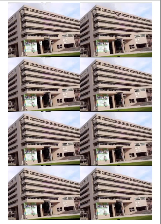
Figure 17: Four iterations of our method with structure enhancement. Top to bottom: iteration 1 to 4.

37

Figure 18: Fourth iteration of one view in Figure 17.

Figure 19: Comparison of three approaches.

Left to right: Original stereoscopic inpainting, our method without structure enhancement, our method with structure enhancement.

38

39

Figure 21: Four iterations of original stereoscopic inpainting. Top to bottom: iteration 1 to 4.

40

41

Figure 23: Four iterations of our method without structure enhancement. Top to bottom: iteration 1 to 4.

42

43

Figure 25: Four iterations of our method with structure enhancement. Top to bottom: iteration 1 to 4.

44

Figure 26: Fourth iteration of one view in Figure 25.

Figure 27: Comparison of three approaches.

Left to right: Original stereoscopic inpainting, our method without structure enhancement, our method with structure enhancement.

45

46

Figure 29: Four iterations of original stereoscopic inpainting. Top to bottom: iteration 1 to 4.

47

48

Figure 31: Four iterations of our method without structure enhancement. Top to bottom: iteration 1 to 4.

49

50

Figure 33: Four iterations of our method with structure enhancement. Top to bottom: iteration 1 to 4.

51

Figure 34: Fourth iteration of one view in Figure 33.

Figure 35: Comparison of three approaches .

Left to right: Original stereoscopic inpainting, our method without structure enhancement, our method with structure enhancement.

52

53

Figure 37: Four iterations of original stereoscopic inpainting. Top to bottom: iteration 1 to 4.

54

55

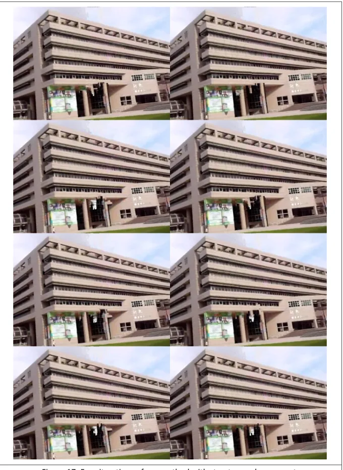
Figure 39: Four iterations of our method without structure enhancement. Top to bottom: iteration 1 to 4.

56

57

Figure 41: Four iterations of our method with structure enhancement. Top to bottom: iteration 1 to 4.

58

Figure 42: Fourth iteration of one view in Figure 41.

Figure 43: Comparison of three approaches.

Left to right: Original stereoscopic inpainting, our method without structure enhancement, our method with structure enhancement.

59

7.2 Discussion

We showed results of different input stereo images. The backgrounds of these images are structural artificiality. Different types of obstacle are marked by user and removed from the images. The image completion results of the original stereoscopic inpainting are showed in Figure 13, 21, 29, 37. We can see the perspective artifacts on the connection of structure line still remain after four iterations of inpainting. Using our method without structure enhancement leads to more reasonable results (Figure 15, 23, 31, 39). The perspective artifacts are effectively reduced but some ghost effects showed up in Figure 16 and Figure 32. Using structure enhanced patch searching in our method, the ghost effects are eliminated (Figure 18 and Figure 34) and the structure of the background is better preserved (Figure 19, 27, 35, 43).

60

Chapter 8

Conclusion

We proposed an automatic image completion method for architectural scene images. Our system takes stereo images and disparity maps as input. Foreground obstacles are defined by users. The stereoscopic inpainting scheme is used for reducing removed pixels from two-view information and detecting unreliable filling pixels. The unreliable pixels are re-inpainted to preserve parallax consistency of stereo images. Since human eyes are sensitive to the structure of artificiality, we improved the inpainting algorithm using vanishing point and vanishing line prediction to project the image to perspective corrected space. Exemplar-based inpainting is performed on the perspective corrected space, and the perspective artifacts are effectively alleviated. We also applied a structure-enhanced patch searching method to exemplar-based inpainting to better preserve the structure of buildings. The results of our method are reasonable and natural.

61

References

[ADV03] A. Almansa,A. Desolneux, S. Vamech. “Vanishing point detection without any a priori information,” IEEE Transactions on Pattern Analysis and Machine Intelligence, Vol. 25, Issue 4, pp. 502-507, 2003.

[ALC05] D. G. Aguilera, J. G. Lahoz, J. F. Codes, “A new method for vanishing points detection in 3d reconstruction from a single view,” Proceedings of the ISPRS Commission, 2005.

[BAR83] S. T. Barnard, “Interpreting perspective images,” Artificial Intelligence 21, pp.435-462, 1983.

[BAR02] W. A. Barrett and A. S. Cheney, “Object-based image editing,” ACM Transactions on Graphics, Vol. 21, Issue 3, pp. 777-784, 2002.

[BBS01] M. Bertalmio, A. L. Bertozzi, G. Sapiro, “Navier-stokes, fluid dynamics, and image and video inpainting,” Computer Vision and Pattern Recognition, Vol. 1, pp. 355-362, 2001.

[BCV01] C. Ballester, V. Caselles, J. Verdera, M. Bertalmi, G. Sapiro, “A Variational Model for Filling-In Gray Level and Color Images,” International Conference on Computer Vision, Vol. 1, pp.10, 2001.

62

[BHA07] P. Bhat, C. L. Zitnick, N. Snavely, A. Agarwala, M. Agrawala, M. Cohen, B. Curless, S. Bing, “Using Photographs to Enhance Videos of a Static Scene,” Symposium A Quarterly Journal In Modern Foreign Literatures, pp. 327–338, 2007.

[BSC00] M. Bertalmio, G. Sapiro, V. Caselles, C. Ballester, “Image inpainting,” SIGGRAPH, pp. 417-424, 2000.

[BVS03] M. Bertalmio, L. Vese, G. Sapiro, S. Osher, “Simultaneous structure and texture image inpainting,” IEEE Transactions on Image Processing, Vol. 12, no. 8, pp. 882-889, 2003.

[CAN86] J. Canny, “A computational approach to edge detection,” IEEE Trans. on Pattern Analysis and Machine Intelligence, Vol. 8, pp. 679–698, 1986.

[CHA01] T. F. Chan and J. Shen, “Nontexture Inpainting by Curvature-Driven Diffusions,” Journal of Visual Communication and Image Representation, Vol. 12, Issue 4, pp. 436-449, 2001.

[CHA02] T. F. Chan, S. Soatto, “Inpainting from Multiple Views,” Proceedings First International Symposium on 3D Data Processing Visualization and Transmission, Vol. 1, pp. 622-625, 2002.

[COM02] D. Comaniciu, P. Meer, “Mean shift: A robust approach toward feature space analysis.” Ieee Trans. On Pattern Analysis and Machine Imtelligence, Vol. 24, Issue 5, pp. 603-619, 2002

63

[CPT03] A. Criminisi, P. Pérez, K. Toyama, “Object removal by exemplar-based inpainting,” IEEE Computer Society Conference on Computer Vision and Pattern Recognition, Vol. 2, pp. II-721-II-728, 2003.

[CY99] J. M. Coughlan and A. L. Yuille, “Manhattan world : Compass direction from a single image by Bayesian inference,” In International Conference on Computer Vision, 1999

[CY03] J. M. Coughlan and A. L. Yuille, “Manhattan world :Orientation and outlier detection by Bayesian inference,” Neural Computation, Vol. 15, no. 5, pp. 1063-1088, 2003.

[DCY03] I. Drori, D. Cohen-Or, H. Yeshurun, “Fragment-based image completion,” ACM Transactions on Graphics, Vol. 22, Issue 3, pp. 303, 2003.

[DOH72] Duda, R. O. and P. E. Hart, “Use of the Hough Transformation to Detect Lines and Curves in Pictures,” Comm. ACM, Vol. 15, pp. 11–15, January, 1972

[DVL06] P. Darko, S. Volker and K. Leif, “Interactive image completion with perspective correction.” The Visual Computer, Vol. 22, Issue 9, pp. 671-681, 2006

[FIS81] M. A. Fischler, R. C. Bolles. “Random sample consensus: A paradigm for model fitting with applications to image analysis and automated cartography.” Communications of the ACM, Vol. 24, Issue 6, pp. 381-395, 1981

[GON03] M. Gong, Y. Yang, “Fast stereo matching using reliability-based dynamic programming and consistency constraints.” Int. Conf. on Computer Vision, pp. 610-617, 2003

64

[HAY07] J. Hays and A. A. Efros, “Scene completion using millions of photographs,” ACM Transactions on Graphics, Vol. 26, Issue 3, pp. 4, 2007.

[MAS98] S. Masnou and J. M. Morel, “Level lines based disocclusion,” Int. Conf. Image Processing, Vol. III, pp. 259-263, 1998.

[MMB97] W. R. Mark, L. McMillan, G. Bishop, “Post-Rendering 3D Warping.” Symp. On Interactive 3D Graphics, pp. 7-16, 1997

[PSK06] D. Pavić, V. Schönefeld, L. Kobbelt. “Interactive image completion with perspective correction,” The Visual Computer, Vol. 22, Issue 9, pp. 671-681, 2006.

[SYJ05] J. Sun, L. Yuan, J. Jia, H. Y. Shum. “Image completion with structure propagation,” ACM Transactions on Graphics, Vol. 24, Issue 3, pp. 861, 2005.

[WAN08] L. Wang, J. Hailin, Y. Ruigang, G. Minglun “Stereoscopic inpainting: Joint color and depth completion from stereo images,” IEEE Conference on Computer Vision and Pattern Recognition, pp. 1-8, 2008.

[WBT05] M. Wilczkowiak, G. J. Brostow, B. Tordoff, R. Cipolla, “Hole Filling Through Photomontage,” Proc British Machine Vision, pp. 492–501, 2005.