以貝氏一致性方法評估銜接性試驗

國

立

交

通

大

學

統計學研究所

碩

碩

碩

碩

士

士

士

士

論

論

論

論

文

文

文

文

以貝氏一致性方法評估銜接性試驗

A Bayesian Consistency Approach to Evaluation

of Bridging Studies

研 究 生：許為翔

指導教授：蕭金福 教授

中

中

中

中

華

華

華

華

民

民

民

民

國

國

國

國

一

一

一

一

百

百

百

百

年

年

年

年

六

六

六

六

月

月

月

月

以貝氏一致性方法評估銜接性試驗

A Bayesian Consistency Approach to Evaluation

of Bridging Studies

研 究 生：許為翔 Student：Wei-Hsiang Hsu

指導教授：蕭金福 Advisor：Chin-Fu Hsiao

國 立 交 通 大 學

統計學研究所

碩 士 論 文

A Thesis

Submitted to Institute of Statistics College of Science

National Chiao Tung University in partial Fulfillment of the Requirements

for the Degree of Master

in

Statistics

June 2011

Hsinchu, Taiwan, Republic of China

以貝氏一致性方法評估銜接性試驗

研究生: 許為翔 指導教授: 蕭金福 博士

國立交通大學統計學研究所 中文 中文中文 中文摘要摘要摘要 摘要 銜接性試驗(bridging study)是全球化藥物發展之一大重要臨床試驗設計，此概念 源自於 1998 年國際醫藥法規機構(International Conference on Harmonization)所建 立之 ICH E5 發展而來。E5 的主題為「Ethnic Factors in the Acceptability of Foreign

Clinical Data」，其目的主要是藉由評估種族因素於藥物效能上的衝擊，繼而協助 藥物於 ICH 區域上市。根據 ICH E5 的定義，當某種新藥已經在某一地區證實其 有效性、安全性且上市之後，此種新藥如要在另一地區註冊上市，而在當地所執 行新藥的臨床試驗，此種試驗便稱為銜接性試驗。由於政府對於國外新藥的引進， 自 2004 年開始，必須先執行銜接性臨床試驗的評估，由此可見銜接性臨床試驗 的研究之重要性。Tsou. et al.(2007)提出了一個貝氏方法合併銜接性試驗和國外臨 床數據來估計兩區域的相似性。然而，即使兩個區域皆具有正向的藥效反應，它 們兩者之間的藥效依舊有可能不相似。因此，在本文中，我們提出一個貝氏一致 性方法來評估兩區域藥效的相似性。另外我們也建立統計理論來計算銜接性試驗 所需要的樣本數。並用例子說明在不同的情況下，如何應用我們提出的方法。 關鍵字 關鍵字 關鍵字 關鍵字: 銜接性試驗,貝氏方法, 一致性, 相似性

A Bayesian Consistency Approach to Evaluation of Bridging Studies

Student: Wei-Hsiang Hsu Advisor: Dr. Chin-Fu Hsiao

Institute of Statistics National Chiao Tung University

Abstract

In 1998, the International Conference on Harmonization (ICH) published a guidance to facilitate the registration of medicines among ICH regions including European Union, the United States of America, and Japan by recommending a framework for evaluating the impact of ethnic factors on a medicine’s effect such as its efficacy and safety at a particular dosage and dose regimen (ICH E5, 1998). The purpose of ICH E5 is not only to evaluate the ethnic factor influence on safety, efficacy, dosage and dose regimen, but also more importantly to minimize duplication of clinical data allow extrapolation of foreign clinical data to a new region. Tsou et al. (2007) have proposed a Bayesian approach to synthesize the data generated by the bridging study and foreign clinical data generated in the original region for assessment of similarity based on superior efficacy of the test product over a placebo control. However, for Tsou et al. (2007), even if both regions have positive treatment effect, their effect sizes might in fact be different. That is, their approach could not truly assess the similarity between two regions. Therefore, in this article we develop a Bayesian consistency approach for assessment of similarity between a bridging study conducted in a new region and studies conducted in the original region. Methods for sample size determination for the bridging study are also proposed. Numerical examples illustrate applications of the proposed procedures in different scenarios.

誌謝

誌謝

誌謝

誌謝

經過研究所兩年的磨練與學習，並且順利完成這篇論文，首要感謝的是指導 教授蕭金福老師。感謝蕭金福老師在忙碌的工作中依舊能夠細心指導我，並帶領 我學習臨床領域的相關知識。同時感謝鄒小蕙老師經常給予協助和指導我研究的 方向，以及蕭老師的研究助理談得聖學長常提出不同的看法，使我更具有多方面 的思維。另外，亦要感謝口試委員陳鄰安老師、黃郁芬老師和林培生老師的指導 與修正，才能使這篇論文更加嚴謹與完善。 感謝交大統計所老師的指導，讓我能順利完成碩士學位。在統計所這兩年， 不僅從老師的課程中學到各種專業的知識，也在和同學討論的過程中，慢慢了解 如何思考與解決各種問題。系上的資源以及學長姐所分享的經歷，亦給予我未來 人生規畫的方向。 最後感謝父母親的辛苦，讓我沒有顧慮的修讀碩士學位，和各位同學、朋友 的陪伴，使我在研究所生涯裡留下許多深刻的回憶。在此，由衷感謝你們溫暖的 陪伴與鼓勵。 為翔 謹誌于 國立交通大學統計學研究所 中華民國一百年六月

Content

中文摘要... i Abstract ... ii 誌謝... iii Content ... iv List of Tables ... iv 1. Introduction ... 1

2. The Bayesian Consistency Approach ... 4

3. Determination of Sample Size ... 9

4. Examples ... 11 5. Discussion ... 14 References ... 16 Appendix ... 28

List of Tables

Table 1 ... 18 Table 2 ... 20 Table 3 ... 21

1. Introduction

In recent years, the possible influence of ethnic factors on clinical outcomes for evaluation of efficacy and safety of study medications under investigation has attracted much attention from both the pharmaceutical/biotechnology industry and the regulatory agencies such as the United States (US) Food and Drug Administration (FDA), especially when the sponsor is interested in bringing an approved drug product from the original region such as the US or European Union (EU) to a new region (e.g., Asian Pacific Region). However, the key issues lie on when and how to address the geographic variations of efficacy and safety for the product development. After a pharmaceutical product has been approved for commercial marketing in one region (e.g., the US or EU) based on its proven efficacy and safety, the pharmaceutical sponsor might seek registration of the product in a new region (Asian Pacific Region). However, the differences in race, diet, environment, culture, and medical practice among regions may have an impact on the extrapolation of the clinical outcomes from the original region to the new region. To address this issue, the International Conference on Harmonisation (ICH) published a guideline entitled “Ethnic Factors in the Acceptability of Foreign Clinical Data” in 1998. This guideline is known as ICH E5 (ICH, 1998). The ICH E5 guideline provides a general framework for evaluation of the impact of ethnic factors on the efficacy, safety, dosage, and dose regimen.

As indicated in the ICH E5 guideline, a bridging study is defined as a study performed in the new region to provide pharmacokinetic (PK), pharmacodynamic (PD), or clinical data on efficacy, safety, dosage, and dose regimen in the new region that will

allow extrapolation of the foreign clinical data to the population in the new region. The ICH E5 guideline suggests the regulatory authority of the new region to assess the ability to extrapolate foreign data based on the bridging data package, which consists of (1) information including PK data and any preliminary PD and dose-response data from the complete clinical data package (CCDP) that is relevant to the population of the new region and if needed, (2) bridging study to extrapolate the foreign efficacy data and/or safety data to the new region. The ICH E5 guideline indicates that bridging studies may not be necessary if the study medicines are insensitive to ethnic factors. For medicines characterized as insensitive to ethnic factors, the type of bridging studies (if needed) will depend upon experience with the drug class and upon the likelihood that extrinsic ethnic factors could affect the medicine’s safety, efficacy, and dose-response. On the other hand, for medicines that are ethnically sensitive, bridging study is usually needed since the populations in two regions are different. In the ICH E5 guideline, however, no criteria for assessment of the sensitivity to ethnic factors for determining whether a bridging study is needed are provided. Moreover, when a bridging study is conducted, the ICH guideline indicates that the study is readily interpreted as capable of bridging the foreign data if it shows that dose-response, safety, and efficacy in the new region are similar to those in the original region. However, the ICH does not clearly define the similarity.

Shih (2001) interpreted similarity as consistency among study centers by treating the new region as a new center of multicenter clinical trials. Under this definition, Shih (2001) proposed a method for assessment of consistency to determine whether the study is capable of bridging the foreign data to the new region. Alternatively, Shao and Chow (2002) proposed the concepts of reproducibility and generalizability

probabilities for assessment of bridging studies. If the influence of the ethnic factors is negligible, then we may consider the reproducibility probability to determine whether the clinical results observed in the original region are reproducible in the new region. If there is a notable ethnic difference, the generalizability probability can be assessed to determine whether the clinical results in the original region can be generalized in a similar but slightly different patient population due to the difference in ethnic factors. Lan et al. (2005) introduced the weighted Z-tests in which the weights may depend on the prior observed data for the design of bridging studies. Note that other methods such as based on similarity in terms of equivalence and non-inferiority have also been proposed in literature (Chow, Shao, and Hu, 2002; Hung, 2003).

One of the crucial reasons for the ICH E5 guideline to emphasize on minimizing unnecessary duplication of generating clinical data in the new region is that sufficient information on efficacy, safety, dosage and dose regimen has been already generated in the original region and is available in the CCDP. One should therefore borrow “strength” from the information on dose response, efficacy, and safety from the CCDP in the original region and incorporate them into the analysis of the additional data obtained from the bridging study. Liu, Hsiao, and Hsueh (2002) have proposed a Bayesian approach to synthesize the data generated by the bridging study and foreign clinical data generated in the original region for assessment of similarity based on superior efficacy of the test product over a placebo control. However, the results of the bridging studies using this approach will be overwhelmingly dominated by the results of the original region due to an imbalance of sample sizes between the regions. In other words, it is very difficult, if not impossible, to reverse the results observed in the original region even the result of the bridging study is not consistent with those of

the original region. However, this issue will occur for any methods for cross-study comparisons if the amount of information is seriously imbalanced between studies. To conquer this problem, Hsiao et al. (2007) then proposed a Bayesian approach with the use of a mixture prior for assessment of similarity between the new and original region based on the concept of positive treatment effect. For both approaches, even if both regions have positive treatment effect, their effect sizes might in fact be different. That is, their approach could not truly assess the similarity between two regions. Therefore, in this thesis we propose a Bayesian approach in which similarity between the new and original region will be concluded if the treatment effect for new region is more than a fraction of the treatment effect for original region trial.

This thesis is organized as follows. In Section 2, a Bayesian consistency approach for assessment of similarity is suggested. The method for sample size determination is given in Section 3. A numerical example is presented in Section 4 to illustrate the Bayesian approach. Discussion and final remarks are given in Section 5.

2. The Bayesian Consistency Approach

For simplicity, we only focus on the trials for comparing a test product and a placebo control. We consider the problem for assessment of similarity between the new and original region based on superior efficacy of the test product over a placebo control. Let X and _Oi Y_Ojbe some efficacy responses for patients i and j receiving the test product and the placebo control respectively in the original region. For simplicity, both XOi’s and YOj’s are normally distributed with variance σ2. We assume that σ2 is

known, although it can generally be estimated. Let µOT and µOP be the population

means of the test and placebo, respectively, and let ∆O = µOT –µOP. The subscript O in

µOT, µOP, and ∆O indicates the original region.

Similarly, let X and _Ni Y_Njbe some efficacy responses for patients i and j receiving the test product and the placebo control respectively in the new region. Again we assume that both XNi’s and YNj’s are normally distributed with known variance σ2. Let

µNT and µNP be the population means of the test and placebo, respectively, and let ∆N

= µNT –µNP. The subscript N in µNT, µNP,and ∆N indicates the new region.

Under the situation that the test product has been already approved in the original region due to its proven efficacy against placebo control, if the data collected from the bridging study show that the efficacy of the test product from the new region is more than a fraction of the efficacy of the test product from the original region, then the efficacy observed in the bridging study in the new region can be claimed to be similar to that of the original region. This concept of similarity is referred to as similarity between the treatment effects from both new and original regions.

Let π_O and π_N represent the priors of ∆O and ∆N respectively. Since the clinical

trial conducted in the original region has been completed, we assume that ∆O has a

non-informative prior. For convention, we assume that ∆O≡1. On the other hand, we

assume that π_N is a mixture normal model as given below

N( N) 1 O( O) (1 1) ( N)

π ∆ =γ π ∆ + −γ π ∆ , (1)

where 0≤ ≤γ₁ 1. In (1), π( )⋅ is a normal prior with mean µ₀ and variance 2 0

summarizing the foreign clinical data about the treatment difference provided in the CCDP. The proposed mixture model of the prior information for ∆N in (1) indicates

that a γ1 value of 0 indicates that the prior π is equivalent to the prior used in Liu,

Hsiao and Hsueh (2002), while γ1 being 1 indicates that no strength of the evidence

for the efficacy of the test product relative to placebo provided by the foreign clinical data in the CCDP from the original region would be borrowed. The choice of weight,

γ1, should reflect relative confidence of the regulatory authority on the evidence

provided by the bridging study conducted in the new region versus those provided by the original region. It should be determined by the regulatory authority of the new region by considering the difference in both intrinsic and extrinsic ethnical factors between the new and original regions. We further assume that π_O and π_N are independent.

Let nOT and nOP represent the numbers of patients studied for the test product and the

placebo respectively in original region, and nNT and nNP the numbers of patients

studied for the test product and the placebo respectively in new region. Based on the clinical responses from the clinical trial in the original region and the bridging study in the new region, ∆O and ∆N can be estimated by

O O O ˆ _{x y} ∆ = − , and N N N ˆ _{x y} ∆ = − , where OT O O 1 n i i x x = =

∑

, OP O O 1 n i i y y = =

∑

, NT N N 1 n i i x x = =

∑

, and NP N N 1 n i i y y = =

∑

. Subsequently, we can derive that

∆ˆ_O∼ N(∆_O, σ_O2) and ∆ˆ_N ∼N(∆_N, σ_N2), where _O2 2 OT OP 1 1 ( ) n n σ = + σ , _N2 2 NT NP 1 1 ( ) n n

σ = + σ , and N( , µ υ2)represents a normal distribution with mean µ and variance υ2

. The marginal density of ∆ˆ_O is

O(ˆO) 1.

m ∆ ≡

On the other hand, the marginal density of ∆ˆ_N can be expressed as

2 N 0 N N 1 1 _{2 2} 2 2 0 N 0 N ˆ ( ) 1 ˆ ( ) (1 ) exp 2( ) 2 ( ) m γ γ µ υ σ π υ σ  _{∆ −}    ∆ = + − −  +   +   (2)

The derivation of equation (2) is described in details in Appendix. Consequently, given the original data and prior information, the posterior distribution of ∆O is

2 O( O|ˆO) N(ˆO, O)

π ∆ ∆ ≡ ∆ σ .

Similarly, given the bridging data and prior information, the posterior distribution of

∆N is 2 N N N N N 1 ₂ 2 N N N N 2 2 N N N 0 1 _{2 2} 2 2 N 0 N 0 ˆ ( ) 1 1 ˆ ( | ) exp ˆ ₂ ( ) 2 ˆ ( ) ( ) 1 (1 ) exp 2 2 2 m π γ σ πσ µ γ σ υ π σ υ  _{ ∆ − ∆ }  ∆ ∆ ≡ _ −  ∆ _     _{∆ − ∆ ∆ −}   _ + − − −      _ (3)

Therefore, the posterior distribution of (∆ ∆_O, _N)is equal to

πO(∆ ∆O|ˆO)πN(∆ ∆N| ˆN). (4)

Given the original data, the data from the bridging study, and prior informations, similarity on efficacy between the new region and the original region can be

concluded if the posterior probability of similarity N 2 O SP N 2 O O O O N N N O N { }

P P( | original data, bridging data, and priors)

ˆ ˆ ( | ) ( | ) 1 , d d γ γ π π τ ∆ > ∆ = ∆ > ∆ = ∆ ∆ ∆ ∆ ∆ ∆ > −

∫

(5)

for some pre-specified 0 <τ< 0.5. However, τ is determined by the regulatory agency of the new region and should generally be smaller than 0.2 to ensure that posterior probability of similarity is at least 80%. Also γ₂ represents the magnitude of consistency trend. Selection of the magnitude, γ₂, of consistency trend should also reflect relative confidence of the regulatory authority on the evidence provided by the bridging study conducted in the new region versus those provided by the original region. Again it should be determined by the regulatory authority of the new region by considering the difference in both intrinsic and extrinsic ethnical factors between the new and original regions.

Since the test product has been already approved in the original region due to its proven efficacy against placebo control, the posterior probability of similarity in (5) can be expressed as N 2 O 2 0 SP O O O N N N O N { } N N N N O O O O ˆ ˆ P ( | ) ( | ) ˆ ˆ ( | ) ( | ) . d d d d γ γ π π π π ∆ > ∆ ∞ ∞ −∞ ∆ = ∆ ∆ ∆ ∆ ∆ ∆   = _ ∆ ∆ ∆ _ ∆ ∆ ∆

∫

∫ ∫

3. Determination of Sample Size

Let nN represent the numbers of patients studied per treatment in the new region.

Based on the discussion in the previous section, the marginal density of ∆ˆ_N in (2) can be re-expressed as 2 N 0 N N 1 1 ₂ 2 2 2 0 0 N N ˆ ( ) 1 ˆ ( ) (1 ) exp 2 2 _{2( )} 2 ( ) m n n µ γ γ σ σ _υ π υ    _{∆ −}    ∆ = + − −   ₊  + _{ }   . (6)

The posterior distribution of∆_N, is therefore, given by

2 N N N N N 1 ₂ 2 N N N N 2 2 N N N 0 1 ₂ 2 2 0 2 0 N N ˆ ( ) 1 1 ˆ ( | ) exp ˆ ₂ ( ) ₂ 2( ) 2 ( ) ˆ ( ) ( ) 1 (1 ) exp 2 2 2 _{2( )} 2 ( ) m n n n n π γ σ σ π µ γ σ υ σ π υ  _{ }  _{ } ∆ − ∆    ∆ ∆ ≡ _ −  ∆ _    _ _       _{∆ − ∆ ∆ −}    + − − − _  _     _ (7)

Given τ, γ₁, γ₂, µ₀, υ₀2, σ2, and the estimate∆ˆ_N, we can determine the sample size nN by finding the smallest nN such that the equation

SP

P > −1 τ, is satisfied.

One approach to determination of ∆N for sample size estimation of the bridging study

is to adopt the “worst outcome criteria” approach suggested by Lawrence and Belisle (1997). Assume that nO represents the numbers of patients studied per treatment in the

that both efficacy endpoints of test drug and the placebo group in the original region have the same variance σ2. Consequently, µ₀ can be estimated by the difference in sample means of the original region and 2 2

0 2 / nO

υ = σ can be estimated by the pooled sample variance of mean difference. Hence, once µ₀ and 2

0

υ are determined,

σ2 in (6) can be obtained by 2 O 0 / 2

n υ . Because the test product has been already approved in the original region due to its proven efficacy against placebo control, the ratio of µ₀ to υ₀ is usually greater than 1.96. Following the “worst outcome criteria” approach by Lawrence and Belisle (1997), the estimate of the treatment difference,

N

ˆ

∆ , is chosen to be the lower bound of a 95% confidence interval for ∆N constructed

from µ₀ and 2 0

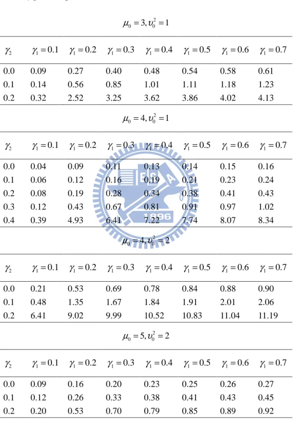
υ . Table 1 provides the ratio of the sample size per treatment group for the bridging study to that of the CCDP ( nN/nO ) for various combination of µ₀

and variance 2 0

υ with τ= 0.2.

From Table 1, the sample size required for the bridging study in the new region decreases as the ratio of µ₀ to υ₀ increase, γ₁ decreases and γ₂ decrease. Therefore, for a given value of µ υ₀/ ₀ , with proper selection of γ₁ and γ₂, reduction of the total sample size for the bridging study is possible when a statistically significant evidence of efficacy for the test product against placebo is provided in the original region.

sample size for the new region is always smaller than that of the original region. This makes intuitive sense since the consistency trend require is not rigid. Also the required sample size per treatment for the bridging study in the new region increases as γ1 increases. For instance, when θ0 = 4, σ02 = 2 (that is, two-side p-value = 0.0455

for the original region), γ2 = 0.1, and τ = 0.2, the sample size required per treatment

for the bridging study increases from 48% of that required in the original region at γ1

=0.1 up to 206% at γ1 = 0.7 with ∆ˆN= 1.23 (the lower bound of a 95% confidence

interval for ∆N constructed given that θ0 = 4 and σ02 = 2). In other words, when less

information borrowed from the original region is incorporated into the prior information, it would require a larger sample size of the bridging study in the new region.

4. Examples

Hypothetical datasets modified from our review experience of bridging studies are used to illustrate the proposed procedure. The CCDP provides the results of three randomized, placebo controlled trials for a new antidepressant (test drug) conducted in the original region. The design, inclusion, exclusion criteria, dose, and duration of these three trials are similar, and hence the three trials constituted as the pivotal trials for approval in the original region. The primary endpoint is the change from baseline of sitting diastolic blood pressure (mmHg) at week 12. Because the regulatory agency in the new region still has some concerns in ethnic differences, both intrinsically and extrinsically, a bridging study was conducted in the new region to compare the difference in efficacy between the new and original region. Two cases with various

probabilities, which is described in the previous section, are considered in this example. For each case, there are three scenarios to be considered. The first scenario presents the situation where no statistically significant difference in the primary endpoint exists between the test drug and placebo. The second situation is that the mean reduction of sitting diastolic blood pressure at week 12 of the test drug is statistically significantly greater than the placebo group. The third scenario is the situation where duo to the insufficient sample size of the bridging study, no statistical significance is found between the test drug and placebo although the magnitude of the difference between the test drug and placebo observed in the original region is preserved in the new region. The number of patients and mean reduction and standard deviations of sitting diastolic blood pressure are provided in Table 2. The Three scenarios are denoted as New 1(Example 1), New 2(Example 2), and New 3(Example 3), respectively.

Using the technique of meta-analysis in Pettiti (2000) to integrate the results from the original regions, we derived that µ0= −13.86 and

2

0 0.58

υ = . For the first two scenarios of the bridging studies considered here, σˆN2 =3.75 for estimation of

2 N

σ ,

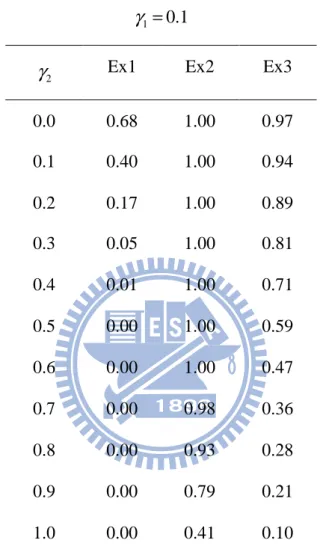
while σˆN2 =14.39 for estimation of 2 N

σ in the last scenario. Table 3 provides the values of PSP with various values of γ1 and γ2 for all three scenarios.

For Example 1, the difference in mean reduction of sitting blood pressure between the test drug and placebo is 0.9 mmHg which is strikingly different from those obtained from three trials conducted in the original region. Hence, when γ1 is not zero (for

example,γ1=0.1), PSP is always less than 80% regardless of the choice of γ2.

Accordingly, we can not conclude that the results of the new region are similar to those of original region. With proper selection of γ1, our proposed procedure reaches a

conclusion that is more consistent with the evidence provided by the new region.

For Example 2, the difference in the mean reduction of sitting blood pressure between the test drug and placebo is 13 mmHg which is quite consistent with those obtained from the three trials conducted in the original region. Hence, as expected, regardless of the choice of γ1, the posterior probabilities are larger than 0.8 unless γ2 is close to

1. Therefore, we can conclude similarity between the new and original regions while

2

γ is chosen appropriately.

For Example 3, the magnitude of the mean difference is 7, is that, the similar situation in the original region. However, the difference is not statistically significant due to its small sample size and the large variability in the new region. As seen from Table 3, the posterior probability PSP decreases as γ2 increases. The values of PSP are greater

than 0.80 when γ2 is chosen to be less than 0.3 regardless of the choice of γ1. That is,

with the strength of the substantial evidence of efficacy borrowed from the CCDP of the original region, our procedure can prove the similarity of efficacy between the new and the original region when a non-significant efficacy result but with a similar magnitude is observed in the bridging study.

Overall, this example demonstrates that with proper selection of γ1 and γ2 by the

conclusion which is much more in line with the results of the bridging study in the new region.

5. Discussion

In this thesis, a Bayesian consistency method has been suggested to synthesize the data from both the bridging study and the original region for assessment of bridging evidence. In this article, the prior information used is a weighted average of a non-informative prior and a normal prior. With an appropriate choice of weight γ1, the

evaluation of similarity based on the integrated results of the bridging studies in the new region and those from the original region will no longer be overwhelmingly dominated by the results of the original region due to an imbalance of sample sizes between the regions. Also, the similarity criterion is established if the treatment effect for new region is more than a fraction of γ₂ of the treatment effect for original region trial with γ₂>0. With an appropriate selection of γ2 , our approach could truly

assess the similarity of effect sizes between two regions. As demonstrated in Example, similarity between the new and original region will be concluded when the difference in primary endpoint between the test drug and placebo observed in the bridging study is of the same magnitude of that obtained from the original region although it is not statistically significant due to the small sample size of the bridging study. As a result, our proposed procedure not only can reach a conclusion that is more consistent with the results obtained from the bridging study but also can achieve the objective of minimizing duplication of clinical evaluation in the new region as specified in the ICH E5 guidance.

Selection of weight γ1 by the regulatory agency in the new region should consider all

differences in both intrinsic and extrinsic ethnical factors between the new and original regions and at the same time should also reflect their belief on the evidence of efficacy provided in the CCDP of the original region. As mentioned before, a bridging study is conducted in the new region because of concerns on ethnic differences between the new and original regions, therefore, it is suggested that weight γ1 be

greater than 0.

Selection of the magnitude, γ2, of consistency trend may be critical. It may be

determined by the regulatory agency in the specific region. All differences in ethnic factors between the specific region and other regions should be taken into account. However, the determination of γ2 will be and should be different from product to

product, from therapeutic area to therapeutic area and from region to region.

In this thesis, it is assumed that σ2 is known for the sample size calculation. In actual practice, σ2 is not known and should be estimated from some data. In fact, extensive literature of results of similar trials may exist, and thus the variability associated with the primary endpoints can also be found in literature. If the data set used is sufficiently large, the estimate of σ2 can be used in place of the true σ2. On the other hand, when the ethnic difference is notable, we can assume that in the second clinical trial conducted in the new region, the population variance is changed to 2 2

C σ , where 0

C> . In practice, the value of C is usually unknown. We may either consider a maximum possible value of C or a set of C -values to carry out our approach.

References

Chow S. C., Shao J., Hu O. Y. P. (2002). Assessing sensitivity and similarity in bridging studies. Journal of Biopharmaceutical Statistics 12:385-400.

Hsiao C. F., Hsu Y. Y., Tsou H. H. (2007). Use of prior information for Bayesian evaluation of bridging studies. Journal of Biopharmaceutical Statistics 17:109-121.

Hung, H. M. J. (2003). Statistical issues with design and analysis of bridging clinical trial. Presented at the 2003 Symposium on Statistical Methodology for Evaluation of Bridging Evidence, Taipei, Taiwan.

ICH, International Conference on Harmonisation. (1998). Tripartite guidance E5 ethic factors in the acceptability of foreign data. The U.S. Federal Register 83:31790-31796.

Lan K. K. G., Soo Y., (2005). The use of weighted z-tests in medical research. Journal

of Biopharmaceutical Statistics 15:625-639.

Lawrence J., Belisle P. (1997). Bayesian sample size determination for normal means and differences between normal means. The statistician 46:209-226.

Liu J. P., Hsiao C. F., Hsueh H. (2002). Bayesian approach to evaluation of bridging studies. Journal of Biopharmaceutical Statistics 12:401-408.

Pettiti D.B. (2000). Meta-Analysis, Decision Analysis, and Cost-Effectiveness

Analysis. New York: Oxford University Press, pp.119-123.

Shao J., Chow S. C., (2002). Reproducibility probability in clinical trials. Stat Med 21:1727-1742.

Shih W. J. (2001). Clinical trials for drug registrations in Asia-Pacific countries: proposal for a new paradigm from a statistical perspective. Controlled Clinical Trials 22:357-366.

Table 1. The ratio of the sample size per treatment of the bridging study to that of the

clinical trials in the CCDP at τ =0.2 with P for different combinations of _SP

0 µ and 2 0 υ 2 0 3, 0 1 µ = υ = 2 γ γ1=0.1 γ1 =0.2 γ1=0.3 γ1 =0.4 γ1=0.5 γ1=0.6 γ1 =0.7 0.0 0.09 0.27 0.40 0.48 0.54 0.58 0.61 0.1 0.14 0.56 0.85 1.01 1.11 1.18 1.23 0.2 0.32 2.52 3.25 3.62 3.86 4.02 4.13 2 0 4, 0 1 µ = υ = 2 γ γ1=0.1 γ1 =0.2 γ1=0.3 γ1 =0.4 γ1=0.5 γ1=0.6 γ1 =0.7 0.0 0.04 0.09 0.11 0.13 0.14 0.15 0.16 0.1 0.06 0.12 0.16 0.19 0.21 0.23 0.24 0.2 0.08 0.19 0.28 0.34 0.38 0.41 0.43 0.3 0.12 0.43 0.67 0.81 0.91 0.97 1.02 0.4 0.39 4.93 6.41 7.22 7.74 8.07 8.34 2 0 4, 0 2 µ = υ = 2 γ γ1=0.1 γ1 =0.2 γ1=0.3 γ1 =0.4 γ1=0.5 γ1=0.6 γ1 =0.7 0.0 0.21 0.53 0.69 0.78 0.84 0.88 0.90 0.1 0.48 1.35 1.67 1.84 1.91 2.01 2.06 0.2 6.41 9.02 9.99 10.52 10.83 11.04 11.19 2 0 5, 0 2 µ = υ = 2 γ γ1=0.1 γ1 =0.2 γ1=0.3 γ1 =0.4 γ1=0.5 γ1=0.6 γ1 =0.7 0.0 0.09 0.16 0.20 0.23 0.25 0.26 0.27 0.1 0.12 0.26 0.33 0.38 0.41 0.43 0.45 0.2 0.20 0.53 0.70 0.79 0.85 0.89 0.92

2 0 6, 0 2 µ = υ = 2 γ γ1=0.1 γ1 =0.2 γ1=0.3 γ1 =0.4 γ1=0.5 γ1=0.6 γ1 =0.7 0.0 0.05 0.09 0.10 0.11 0.12 0.13 0.13 0.1 0.07 0.12 0.15 0.17 0.18 0.19 0.19 0.2 0.10 0.19 0.25 0.28 0.30 0.32 0.33 0.3 0.16 0.39 0.52 0.59 0.64 0.67 0.70 0.4 0.56 1.84 2.33 2.59 2.75 2.86 2.94 2 0 6, 0 3 µ = υ = 2 γ γ1=0.1 γ1 =0.2 γ1=0.3 γ1 =0.4 γ1=0.5 γ1=0.6 γ1 =0.7 0.0 0.11 0.19 0.24 0.26 0.28 0.29 0.30 0.1 0.17 0.32 0.40 0.44 0.47 0.49 0.51 0.2 0.32 0.70 0.87 0.96 1.01 1.05 1.08 0.3 1.97 3.40 3.90 4.17 4.33 4.43 4.52 2 0 7, 0 3 µ = υ = 2 γ γ1=0.1 γ1 =0.2 γ1=0.3 γ1 =0.4 γ1=0.5 γ1=0.6 γ1 =0.7 0.0 0.07 0.11 0.13 0.14 0.15 0.15 0.16 0.1 0.10 0.16 0.19 0.21 0.22 0.23 0.24 0.2 0.14 0.27 0.33 0.37 0.39 0.41 0.42 0.3 0.28 0.62 0.78 0.86 0.91 0.95 0.98 0.4 2.87 4.94 5.71 6.12 6.37 6.54 6.67 2 0 8, 0 3 µ = υ = 2 γ γ1=0.1 γ1 =0.2 γ1=0.3 γ1 =0.4 γ1=0.5 γ1=0.6 γ1 =0.7 0.0 0.05 0.07 0.08 0.09 0.09 0.09 0.10 0.1 0.06 0.10 0.12 0.13 0.13 0.14 0.14 0.2 0.09 0.15 0.18 0.20 0.21 0.22 0.23 0.3 0.15 0.27 0.34 0.38 0.40 0.42 0.43 0.4 0.34 0.78 0.98 1.09 1.16 1.21 1.24

Table 2. Descriptive statistics of reduction from baseline in sitting diastolic blood

pressure (mmHg)

Treatment group

Region Statistics Drug Placebo

Original 1 N 138 132 Mean -18 -3 Standard deviation 11 12 Original 2 N 185 179 Mean -17 -2 Standard deviation 10 11 Original 3 N 141 143 Mean -15 -5 Standard deviation 13 14 New 1 (Example 1) N 64 65 Mean -4.7 -3.8 Standard deviation 11 11 New 2 (Example 2) N 64 65 Mean -15 -2 Standard deviation 11 11 New 3 (Example 3) N 24 23 Mean -11 -4 Standard deviation 13 13

Table 3 Values of P derived from examples 1,2, and 3 with various values of _SP γ₁

and γ₂

1 0.1

γ =

2

γ Ex1 Ex2 Ex3

0.0 0.68 1.00 0.97 0.1 0.40 1.00 0.94 0.2 0.17 1.00 0.89 0.3 0.05 1.00 0.81 0.4 0.01 1.00 0.71 0.5 0.00 1.00 0.59 0.6 0.00 1.00 0.47 0.7 0.00 0.98 0.36 0.8 0.00 0.93 0.28 0.9 0.00 0.79 0.21 1.0 0.00 0.41 0.10

1 0.2

γ =

2

γ Ex1 Ex2 Ex3

0.0 0.68 1.00 0.97 0.1 0.40 1.00 0.94 0.2 0.17 1.00 0.88 0.3 0.05 1.00 0.79 0.4 0.01 1.00 0.68 0.5 0.00 1.00 0.55 0.6 0.00 0.99 0.42 0.7 0.00 0.97 0.30 0.8 0.00 0.90 0.21 0.9 0.00 0.73 0.14 1.0 0.00 0.39 0.07

1 0.3

γ =

2

γ Ex1 Ex2 Ex3

0.0 0.68 1.00 0.97 0.1 0.40 1.00 0.93 0.2 0.17 1.00 0.87 0.3 0.05 1.00 0.78 0.4 0.01 1.00 0.67 0.5 0.00 1.00 0.53 0.6 0.00 0.99 0.40 0.7 0.00 0.96 0.28 0.8 0.00 0.88 0.18 0.9 0.00 0.69 0.12 1.0 0.00 0.37 0.06

1 0.4

γ =

2

γ Ex1 Ex2 Ex3

0.0 0.68 1.00 0.97 0.1 0.40 1.00 0.93 0.2 0.17 1.00 0.87 0.3 0.05 1.00 0.78 0.4 0.01 1.00 0.66 0.5 0.00 1.00 0.52 0.6 0.00 0.99 0.39 0.7 0.00 0.96 0.26 0.8 0.00 0.86 0.17 0.9 0.00 0.66 0.10 1.0 0.00 0.36 0.05

1 0.5

γ =

2

γ Ex1 Ex2 Ex3

0.0 0.68 1.00 0.97 0.1 0.40 1.00 0.93 0.2 0.17 1.00 0.87 0.3 0.05 1.00 0.78 0.4 0.01 1.00 0.66 0.5 0.00 1.00 0.52 0.6 0.00 0.99 0.38 0.7 0.00 0.96 0.26 0.8 0.00 0.85 0.16 0.9 0.00 0.65 0.09 1.0 0.00 0.36 0.05

1 0.6

γ =

2

γ Ex1 Ex2 Ex3

0.0 0.68 1.00 0.97 0.1 0.40 1.00 0.93 0.2 0.17 1.00 0.87 0.3 0.05 1.00 0.78 0.4 0.01 1.00 0.65 0.5 0.00 1.00 0.51 0.6 0.00 0.99 0.37 0.7 0.00 0.95 0.25 0.8 0.00 0.84 0.16 0.9 0.00 0.63 0.09 1.0 0.00 0.35 0.04

1 0.7

γ =

2

γ Ex1 Ex2 Ex3

0.0 0.68 1.00 0.97 0.1 0.40 1.00 0.93 0.2 0.17 1.00 0.87 0.3 0.05 1.00 0.77 0.4 0.01 1.00 0.65 0.5 0.00 1.00 0.51 0.6 0.00 0.99 0.37 0.7 0.00 0.95 0.25 0.8 0.00 0.84 0.15 0.9 0.00 0.62 0.08 1.0 0.00 0.35 0.04

Appendix

We can derive that

( )

(

)

(

)

(

)

(

)

(

)

(

)

(

)( )

2 N N N N ₂ 2 N N 2 N 0 1 1 ₂ 2 N 0 0 2 2 N N _{N 0} 1 1 ₂ 2 ₂ 2 N N 0 N 0 1 1 1 ˆ 1 ˆ _exp 2 2 1 1 exp 2 2 ˆ 1 1 1 exp exp 2 2 2 2 1 A m d d σ πσ µ γ γ υ πυ µ γ γ σ υ πσ πυ γ γ ∞ −∞ ∞ −∞  _{∆ − ∆}    ∆ = ⋅ _− _⋅       _{∆ −}   _{+ − ⋅} ₋  _∆    _{ }    _{∆ − ∆}  _{ } ∆ −   = + − ⋅ _− _⋅ ⋅ −  ∆     _{ }   = + −

∫

∫

In addition,

( )

(

)

(

)

(

)

(

)

(

)

(

)

2 2 N N _{N 0} 1 ₂ 2 ₂ 2 N N 0 N 0 2 ₂ 2 2 0 N N N N 0 N 2 2 2 2 N 0 N 0 2 2 2 2 2 2 2 2 2 0 N N 0 N 0 N N 0 N N 0 2 2 2 2 N 0 N 0 ˆ 1 1 A exp exp 2 2 2 2 ˆ 1 exp 2 2 ˆ ˆ 2 1 exp 2 2 d d µ σ υ πσ πυ υ σ µ σ υ π σ υ υ σ υ µ σ υ σ µ σ υ π σ υ ∞ −∞ ∞ −∞  _{∆ − ∆}  _{ } ∆ −   = ⋅ _− _⋅ ⋅ −  ∆     _{ }    _{∆ − ∆ + ∆ −}    = _− _ ∆      _{+ ∆ − ∆ + ∆ + ∆ +}    = _−  

∫

∫

(

)

(

)

(

)

N 2 2 2 2 2 2 2 0 N 0 N 0 N N 0 2 2 2 2 2 2 2 2 N 0 N 0 0 N N 0 2 2 2 2 2 2 2 2 0 N 0 N 0 N 0 N 0 N N 2 2 N 2 2 0 N 0 N N 2 2 N 0 ˆ ˆ 1 exp 2 2 2 ˆ ˆ 2 exp 2 d d υ µ σ υ σ µ σ υ σ υ υ σ π σ υ υ µ σ υ µ σ υ σ υ σ υ σ σ υ ∞ −∞ ∞ −∞ ∆   _{∆ +}  ∆ +   = ⋅ _− + _⋅ +       _{∆ +  ∆ + }   ₊ _{∆ − ∆ + }   _{+ +}   _{   } ₋  _∆        

∫

∫

(

)

(

)

(

)

(

)

(

)

(

)

2 2 2 2 2 2 2 2 2 0 N 0 N 0 N 0 N N 0 2 2 2 2 2 2 N 0 0 N N 0 2 2 2 0 N 0 N N 2 2 0 N N 2 2 N 0 2 2 0 N 2 2 2 N 0 _{N 0} 2 2 2 2 2 0 N 0 N N 0 ˆ ˆ 1 exp 2 2 ˆ exp 2 ˆ 2 1 exp 2 2 d υ µ σ υ σ υ σ µ σ υ υ σ π σ υ υ µ σ υ σ σ υ υ σ µ _{πσ υ} υ σ υ σ π σ υ ∞ −∞  _{∆ + − + ∆ +}    = ⋅ _{ }⋅ +      _{ ∆ + }   _{∆ − }  + ₋   _∆     +     _{− ∆ −}    = ⋅ _{ }⋅ + +    

∫

(

)

(

)

(

(

)

)

2 2 N 0 2 2 2 2 0 N 0 N ˆ 1 exp 2 2 µ υ σ π υ σ _{− ∆ −}    = _{ } +   + _{ } Hence,

( )

(

)

(

)

(

(

)

)

2 N 0 N N 1 1 _{2 2} 2 2 0 N 0 N ˆ 1 1 exp 2 2 m γ γ µ υ σ π υ σ _{− ∆ −}    ∆ = + − _{ } +   + _  .