A Hybrid Forecasting Model for Foreign Exchange Rate Based on a Multi-neural Network

(1)

A Hybrid Forecasting Model for Foreign Exchange Rate Based on a Multi-neural

Network

An-Pin Chen

1

, Yu-Chia Hsu

1 2

, Ko-Fei Hu

1

_{Institute of Information Management, National Chiao Tung University, Taiwan,}

2

_{Mackay Medicine, Nursing and Management College, Taiwan}

apc@iim.nctu.edu.tw, hyc0212@gmail.com, coffeehu1212@gmail.com

Abstract

In this work, a multi-neural network model consisting of three sub-networks and one master network is proposed to combine the fundamental theorem and technical analysis in TWD/USD exchange rate forecasting. The long-term, mid-term, and short-term tendencies of exchange rate are forecasted separately by different sub-networks. Five macro economics factors of price level, interest rates, money supply, imports/exports, and productivity, and seven practical technical indicators of fifteen-day and one-day intervals are selected as the input variables of the three sub-networks. The master network then provides the integrated forecasting according to the three sub-networks. To increase forecasting accuracy, a threshold filtering mechanism was applied in this work. The experiment result shows that the multi-neural network is more effective than the random walk model and single-neural network model, and with the threshold filtering, can achieve high accuracy.

1. Introduction

Foreign exchange is one of the most important financial markets for investors. However, since the exchange rate rapidly changes over short time periods and has high volatility, the investor or hedger desires for an effective method to evaluate the dynamic tendency of change and reduce the risk. Although, there are many financial models that have been provided to explain and analyze the behavior of exchange rate, the accuracy of exchange rate forecasting is still an important issue and needs improvement. Many research studies indicate that the non-linear property is observed in exchange rate. Thus, using conventional methodology based on statistics and economics can hardly forecast the exchange rate [1][2][3].

Artificial intelligence is an emerging approach to forecast exchange rate and can achieve acceptable results. Most researchers apply a genetic algorithm or neural network on technical analysis or on fundamental analysis to develop forecasting models. However, only a few studies consider technical and fundamental analysis at the same time.

In this study, a hybrid model which combines fundamental and technical analysis in multi-neural network (MNN) is proposed to forecast exchange rate. In fundamental analysis, the key factors that influence the change tendency of exchange rate were derived from previous literature and economic models. On the other hand, in technical analysis, some commonly used indices and indicators were selected. After data transforming, pre-processing, and filtering, these factors and indicators were fed into the multi-neural network. Compared with the random walk model and three stand-alone neural network models of fundamental and technical analysis, the proposed MNN model is more accurate than others.

This study provides a valuable insight using macro economic time series and technical indicators for MNN. Furthermore, the proposed model can provide the foreign exchange investor with a useful tool to make trading decisions.

The rest of the paper is organized as follows: Section 2 illustrates the methodologies for exchange rate analysis; Section 3 describes the proposed hybrid model and experiment design; Section 4 details the experiment results; and lastly, conclusions drawn from the study will be discussed in Section 5.

2. Methodologies for Foreign Exchange Rate

Analysis

To construct a hybrid forecasting model, the perspectives on fundamental analysis and technical analysis are both considered and discussed, as follows.

2.1. Fundamental Analysis Based on the

Financial Model

Traditionally, classic financial models for foreign exchange analysis are Purchasing Power Parity, Interest Rate Parity, Monetary Approach, Balance of International Payment, and Balassa-Samuelson hypothesis.

Purchasing Power Parity (PPP) was firstly proposed by Gustav Cassel in 1916 to illustrate the relation of price level and exchange rate between two different countries. PPP was wildly evidenced in many empirical studies [4] and indicated that the change of exchange rate is not a Fourth International Conference on Natural Computation

293

Fourth International Conference on Natural Computation

293

(2)

stochastic process [5]. PPP was also used with other theories to forecast exchange rate and obtained better results than the random walk model [6]. Consequently, exchange rate is affected by price level.

Interest Rate Parity was first proposed by John Keynes in 1923, wherein the interest rate of different countries and exchange rate were discussed. If the interest rates of two countries are different and no risk of exchange rate change exists, the arbitrage opportunity would occur. The relative interest rate between two countries is an important factor that will influence the exchange rate.

Monetary Approach was proposed by Mundel in 1963 and suggested that the variation of exchange rate comes from the international capital move. Further, Frankel and Dornbusch proposed the Flexible-price Monetary Model and Sticky-price Monetary Model in 1976 to modify the Monetary Approach. The Flexible-price Monetary Model suggested that the exchange rate is determined by the supply and demand of the currency in two markets, and Sticky-price Monetary Model enhanced the explanation ability of exchange rate volatility in a short period. Hence, currency supply is one of the factors that will influence exchange rate.

Balance of International Payment is the first theorem to explain the variation of exchange rate, which was proposed by Goschen in 1861. The theorem suggested that international payment influences exchange rate. In macro-economics, international payment can be divided into current account and capital account. Capital account is calculated by import value and export value. As a result, exchange rate is affected by import and export values.

The Balassa-Samuelson hypothesis was proposed by Balassa in 1964 and suggested that if productivity is increasing, the wages of the tradable sector is increasing and the wages of the non-tradable sector is also increasing almost immediately. However, the price of the tradable sector is determined by the international market. Thus, the speed of increase in the tradable sector will be slower than that in the non-tradable sector. This will lead to exchange rate increase.

Summarizing the theorems described above, the variation of exchange rate is affected by five factors: price level, interest rate, currency supply, import/export value, and productivity. These five factors are used to construct the forecasting model in this study.

2.2. Technical Analysis in the Financial Market

Technical analysis has been used in practice for forecasting the tendency of the financial market since the 1980s. Many economists, however, challenged the use of technical analysis for market prediction as it cannot make profit due to the Efficient Market hypothesis. On the other hand, some believed that technical analysis can help predict market trend and make profit.

Technical analysis is based on the processing trading price and volume by computing the summation, average, moving average, and smooth into various indicators and index. The most popular technical indicators used in practice and in academic empirical research are Moving Average (MA), Momentum (MTM), Williams Overbought/Oversold Index (%R), Relative Strength Indicator (RSI), Stochastic Indicator (KD), Moving Average Convergence-Divergence (MACD), and Directional Movement Index (DMI).

Some researchers applied these indicators in empirical studies and verified the effectiveness on stick price forecasting with MA [7] [8], exceed return by momentum strategy [9] [10], exceed return in foreign exchange futures market with MA [11], exceed return in USD-JPY and USD-DEM exchange rate with MA [12], and exceed return in foreign exchange market with several technical indicators selected by the Genetic Algorithm [13].

Therefore, technical analysis has the ability to forecast the foreign exchange market and is applied to develop a more accurate and ease-for-practical-use hybrid model in this study.

3. Hybrid Forecasting Model

MNN consists of a master network and several single sub-networks. Each sub-network is linked with the master network with the same weight, but the number of input variables, nodes, and hidden layers in each sub-network are defined independently. Some MNNs have different types of sub-networks and others have the same type. In general, the back-propagation network (BPN) is commonly used in MNNs with the same sub-networks due to its rapid learning speed.

After training, the outcomes of each sub-network according to the inputted values are then fed into the master as the input value. The master network is used for synthesizing the outcomes of sub-networks, which brings the benefits of considering different perspectives when designing sub-networks and inheriting the optimal forecasting results of each sub-network to retrieve more accurate and stable forecasting results.

Therefore, we use MNN to synthesize the fundamental and technical analysis with different time intervals in foreign exchange rate forecasting. The details of MNN components, operation, and the experiment design are described in the following sections.

3.1. Model Architecture Design

In order to consider the fundamental and technical analysis simultaneously, one master network and three sub-networks are used to construct MNN, which is shown in Figure 1. In general, the fundamental analysis uses the macro economics data reported every month to analyze

294 294 294 294

(3)

exchange rate tendency, but technical analysis uses the daily calculated indicators according to the closing price and trading volume. Therefore, we design the three sub-networks to represent the long-term, mid-term, and short-term predictions, respectively.

Master Networks Sub Networks Data bank Data Pre-processing Historical macro economic monthly data Historical exchange rate Data transform

Technique indicators calculation Highest, lowest,

closing price of 15 day interval

Daily closing price

First order differential

Input dataset for sub network III sub-network III (BPN-T1) output dataset of sub network II Integrated forecasting results Input dataset for sub network I Input dataset for sub network II Sub-network II (BPN-T15) Sub-network I (BPN-F) master network (MNN) output dataset of sub network III output dataset of sub network I normalization Identify the change tendency of exchange rate by financial model

split to training data and testing data randomly

Figure 1. Structure design of the forecasting model The long-term prediction which applies the fundamental analysis is performed by sub-network I (BPN-F) in Figure 1. The mid-term and short-term predictions are performed by sub-networks II (BPN-T15) and III (BPN-T1) in Figure 1 by using fifteen-day and one-day data technical indicators, respectively.

The operation of MNN involves the following four processes: (1) data bank, (2) data pre-processing, (3) sub-networks, and (4) master network. First, the macro economics monthly data and the highest, lowest, and closing price of foreign exchange in fifteen-day and one-day intervals are retrieved from the historic data bank. Second, the data are filtered, transformed, or computed in the data pre-processing process and then considered as the input dataset for the three sub-networks. The data are then

split into two groups, training dataset and testing dataset, and then fed to the sub-networks. After the sub-networks are well trained, each one can forecast the long-term, mid-term, and short term tendencies of exchange rate. Finally, the values of long-term, mid-term, and short term tendencies predicted by the sub-networks are taken as the input data of the master network for training and testing. The master network synthesizes the sub-network forecasting to obtain the final exchange rate forecast of the next day.

3.2. Input Variables Selection

In this study, the three sub-networks are used to learn the historical macro economics data and foreign exchange market data. The input variables of the three sub-networks are selected from various economics statistics indicators and foreign exchange trading data in the data bank.

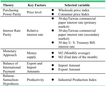
Based on earlier literature described in Section 2.1, five key factors of macro economics (i.e. price level, relative interest rate, money supply, export/ import amount, and productivity), which influence foreign exchange are concluded. We choose 10 indicators, which are appropriate to represent the five key factors as the input variables of BPN-F. These are listed in Table 1.

Table 1. Sub-network I (BPN-F) input variables derived from basic theory

Theory Key Factors Selected variable

Purchasing

Power Parity Price level

z Wholesale price index z Consumer price Index

Interest Rate Parity

Relative interest rate

z 30-dayTaiwan commercial paper interest rate (primary market)

z 30-dayTaiwan commercial paper interest rate (secondary market)

z 30 day U. S. Treasury Bill interest rate

Monetary

Approach Money _supply z M2 (Monthly average) _{z M2 (End date of the month)} Balance of International Payment Export and Import Amounts z Import Amount z Export Amount Balassa-Samuelson

Hypothesis Productivity z Industrial Production Index

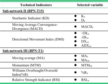
Another two sub-networks are used for technical analysis to forecast the fifteen-day and one-day tendencies. For the fifteen-day forecast, the change properties of exchange rate (i.e. the highest and lowest closing prices) should be considered. Hence, three technical indicators, KD, MACD, and DMI, which are calculated based on the change properties, are adopted for BPN-T15, and four technical indicators, MA, MTM, %R,

295 295 295 295

(4)

and RSI, which are calculated only based on the daily closing price, are adopted for BPN-T1.

The technical indicators selected as input variables for BPN-T15 and BPN-T1 are listed in Table 2. The sampling intervals for indicators calculation are defined based on practical experience. For example, MACD9 means calculate the MACD according to the past nine periods, in other words, use the highest and lowest closing prices during the past nine days and the closing price on current day to calculate MACD.

Table 2. Sub-networks II and III (T15 and BPN-T1) input variables derived from technical analysis

Technical Indicators Selected variable Sub-network II (BPN-T15)

Stochastic Indicator (KD) z K9

z D9

Moving Average

Convergence-Divergence (MACD) z MACD9

Directional Movement Index (DMI)

z +DI14

z -DI14

z DX14

z ADX14

Sub-network III (BPN-T1)

Moving average (MA) z MA5

z MA10

Momentum (MTM) z MTM20

Williams Overbought/Oversold

Index(%R) z %R9

Relative Strength Indicator (RSI) z RSI14

3.3. Data Pre-processing

Besides the input variables for the sub-networks described above, the dynamic behavior of variable change is applied to increase the learning reliability of the neural network. We use the first-order differential expressed in Formula 1 to represent the dynamic behavior, which is commonly used in time series analysis to transform a non-stationary series into a non-stationary one. Consequently, the numbers of total input variables for the three sub-networks are 20, 14, and 10 for BPN-F, BPN-T15, and BPN-T1, respectively. 1 1 ˆ t t t t x x x x − − − = (1) t

xˆ

: First-order differential of input variable at time t

t

x

: Input variable at time t

1 − t

x

: Input variable at time t-1

Moreover, considering the cause and effect relationship between the fundamental macro economics indicators and exchange rate, we suggest to add a binary variable in BPN-F, which represents the stability of the indicator and exchange rate change. If the change

tendencies are the same, the binary variable is 1, else is 0. For example, when the price level is increasing but the exchange rate is decreasing simultaneously, the binary variable is 0. The number of input variables for BPN-F then becomes 30.

Finally, when the data are entered in the sub-networks, the values are normalized between 0 and 1 using the linear function.

3.4. Data and Experiment Design

The data source of the macro economic indicators and TWD/USD exchange rate in this study is the Taiwan Economic Journal Data Bank. Considering the completeness of each economic indicator, the data used for BPN-F is from Jan. 1996 to Dec. 2005 with a total of 121 records. The original data of exchange rate is from 6 Jun. 1988 to 12 Feb. 2007. After sampling and technical indicators calculation, the daily closing price of exchange rate used for BPN-T1 has 5137 records from 30 Jun. 1988 to 24 Jan. 2007, and the fifteen-day sampling data for BPN-T15 has 309 records from 2 Apr. 1990 to 10 Jan. 2007.

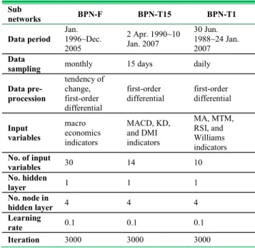
The parameters used in the neural network in this study are determined by referencing from previous research works. We use one hidden layer for all BPN in this study referring to Zhang’s (1998) [14] research, which indicates one hidden layer BPN can satisfy the accuracy and reliability in common use. The number of nodes in the hidden layer is determined by trial and error which is referred from Davies’s (1994) [15] research. We used one to 10 nodes in the hidden layer to test the network and concluded that when the number of nodes is less than three, the error function of the network converges slowly and the when the number of nodes is increased, the learning time will increase but the forecasting result will not be visibly affected. Consequently, we adopt one hidden layer with four nodes in this study.

The learning rate and iteration of the network were also determined by trail and error. After several tests, we find that when the learning rate is one and iteration is 300, the mean square error of the network is less than 0.0000001 in an acceptable learning time. The parameters used for BPN in this study are summarized and listed in Table 3.

The data used in each model were separated randomly into two groups, 80 % of data in the train set and 20 % in the testing set [16]. The random walk model is considered as the control group to compare neural network approaches in this study. A random value between 0 and 1 simulated the output value of the neural network. If the random value is greater than 0.5, the forecasting exchange rate has an uptrend, otherwise a downtrend. The experiments were performed 10 times for each model and

296 296 296 296

(5)

then the average and standard deviation of forecasting accuracy were calculated.

Table 3. Parameters of the BPNs

Sub networks BPN-F BPN-T15 BPN-T1 Data period Jan. 1996~Dec. 2005 2 Apr. 1990~10 Jan. 2007 30 Jun. 1988~24 Jan. 2007 Data

sampling monthly 15 days daily Data pre-procession tendency of change, first-order differential first-order

differential first-order differential

Input variables macro economics indicators MACD, KD, and DMI indicators MA, MTM, RSI, and Williams indicators No. of input variables 30 14 10 No. hidden layer 1 1 1 No. node in hidden layer 4 4 4 Learning rate 0.1 0.1 0.1 Iteration 3000 3000 3000

3.5. Threshold Filtering

In order to eliminate the slight change on exchange rate forecasting to increase the accuracy, a threshold filtering algorithm is proposed in this study:

I. (in training period) Calculate the increase/decrease value of the forecasting exchange rate.

II. Sort the absolute value from I.

III. Set threshold = 10% percentile smallest value from II.

IV. (in testing period) If the absolute value of exchange rate increase/decrease < threshold, then abandon the prediction.

Only the change values greater than the threshold are meaningful and adopted for accuracy calculation.

3.6. Evaluating Scheme

Performance measurement of the proposed model is performed by the accuracy rate of forecasting. If the forecasting exchange rate is increased and the actual exchange rate is also increased, then the forecasting is correct. The accuracy rate is defined, as follows:

g forecastin of number total direction tendency g forecastin of s correctnes rate accuracy ₌ (2)

4. Experiment Results

The experiments were carried out 10 times on the data described in Section 3.4 to calculate the average and standard deviation of the forecasting accuracy (Table 4). All the neural network models can obtain higher accuracy rates than the random walk model. In addition, comparing BPN-F, BPN-T15, and BPN-T1, the fundamental analysis model with monthly indicators (BPN-F) is more accurate than the technical analysis model (BPN-T15, BPN-T1), and the fifteen-day technical indicators (BPN-T15) are more suitable for the BPN model which can attain higher accuracy than one-day indicators (BPN-T1). In order words, the dynamic behavior of exchange rate is appropriate to modeling using long-term indicators by neural networks. The combination forecasting strategy that uses MNN to synthesis the short-term, mid-term, long-term forecasting was also evidenced in Table 4. MNN can increase the forecasting accuracy rate from 59.58 % predictability by BPN-F to 66.82 %.

In our research, we proposed the threshold filtering mechanism to increase forecasting accuracy and Table 4 shows it is effective. The forecasting accuracy rate can be improved about 5.5 % on the average by using threshold filtering, especially 6.9 % in MNN.

Table 4. Accuracy comparison of the forecasting models Forecasting Models Without threshold filtering With threshold filtering Ave. Std. Ave. Std. BPN-F 59.58 % 6.23 % 62.27 % 8.58 % BPN-T15 54.78 % 4.26 % 57.74 % 4.29 % BPN-T1 49.26 % 1.47 % 51.89 % 1.94 % MNN 66.82 % 4.21 % 71.44 % 5.88 % Random walk 47.25 4.97 % N.A. N.A.

5. Conclusion

In this study, we proposed a foreign exchange rate forecasting model based on MNN to predict TWD/USD exchange rate. The basic concept of the proposed model is to integrate fundamental analysis and technical analysis, and consider the long-term, mid-term, and short-term tendencies at the same time. Consequently, MNN consists of a fundamental analysis BPN and two technical analysis BPNs with different time intervals. After empirically studying nearly 19 years of real data, MNN can obtain the highest accuracy rate of 66.82± 4.21% when compared with a single BPN and the random walk model. Furthermore, the threshold filtering mechanism proposed in this study, which can improve forecasting accuracy, can also be evidenced from the experiments.

This research provides a foreign forecasting model which can simulate the dynamic behavior of exchange rate with high accuracy and is valuable for investment and academic research. This computational model can be used not only for developing investment decision support

297 297 297 297

(6)

systems, but also for investigating the key factors that influence the exchange rate by the analysis of the weight of the neural network.

6. References

[1] Pippenger, M.K. and Geppert, J.M., “Testing purchasing power parity in the presence of transactions costs”, Applied

Economics Letters 4 (10), 1997, pp.611–614.

[2] Chen, S. and Wu, J., ”A Re-Examination of Purchasing Power Parity in Japan and Taiwan”, Journal of

Macroeconomics, Vol.22, 2000, pp.271-284.

[3] Ma, Y. and Kanas, A., “Testing for a nonlinear relationship among fundamentals and exchange rates in the ERM”, Journal

of International Money and Finance, Vol.19, 2000, pp.135-152.

[4] Bernhard Heitger,” Purchasing Power Parity under Flexible Exchange Rate – The Impact of Structure Change”, Review of

World Economics, Vol. 123, Issu. 1, 1987, pp.149-156.

[5] Froot, K.A. and Rogoff.K, ”Perspective on PPP and Long-Run Real Exchange Rates”, Handbook of International Economics, Amsterdam, North Holland, 1995, pp. 1647-88. [6] MacDonald, R. & Marsh I.W., “On Fundamentals and Exchange Rate: A Casselian Perspective,” The Review of

Economics and Statistics, Vol.79, 1997, pp.655-664.

[7] Brock, W., Lakonishok, J. and LeBaron, B., ”Simple Technical Trading Rules and the Stochastic Properties of Stock Returns”, Journal of Finance, Vol.47, 1992, pp.1731-1764. [8] Bessembinder, H. and Chan, K, “The Profitability of Technical Trading Rules in the Asian Stock Markets”,

Pacific-Basin Finance Journal, Vol.3, 1995, pp.257-284.

[9] Jegadeesh, N. and Titman, S., “Returns to buying winners and selling losers: Implicatiofor stock market efficiency”,

Journal of Finance, Vol.48, 1993, pp.65-91.

[10] Chan, L. K. C., Jegadeesh, N. and Lakonishok, L., “Momentum strategies”, Journal of Finance, Vol.51, 1996, pp.1681-1713.

[11] Levich, R, and Thomas, L., “The Significance of Technical Trading-Rule Profits in the Foreign Exchange Market: A Bootstrap Approach,” Journal of International Money and

Finance, Vol.12, 1993, pp.563-586.

[12] LeBaron, B., “Technical Trading Rule Profitability and Foreign Exchange Intervention”, Journal of International

Economics, Vol. 49, No. 1, 1999 , pp. 125-143.

[13] Christopher Neely, Paul Weller, and Rob Dittmar, “Is Technical Analysis in the Foreign Exchange Market Profitable? A Genetic Programming Approach”, The Journal of Financial

and Quantitative Analysis, Vol. 32, No. 4. (Dec., 1997), pp.

405-426.

[14] Zhang, G., Patuwo, B. E., & Hu, M. Y., “Forecasting with Artificial Neural Netwroks: The State of the Art”, International

Journal of Forecasting, Vo.14, 1998, pp.35-62.

[15] Davies, P. C., “Design Issues in Neural Network Development”, NEUROVEST Journal, Vol.5, pp.21-25, 1994. [16] Kerns M., ”A bound on the error of cross validation using the approximation and estimation rates, with consequences for the training-test split”, Advance in Neural Information

Processing System, Vol.8, 1996, pp.183-189.

298 298 298 298