Grid-based heuristic method for multifactor landfill siting

Grid-Based Heuristic Method for Multifactor Landfill Siting

Hung-Yueh Lin

and Jehng-Jung Kao, M.ASCE

Abstract: Siting a landfill requires the processing of a large amount of spatial data. However, the manual processing of spatial data is tedious. A geographical information system 共GIS兲, although capable of handling spatial data in siting analyses, generally lacks an optimization function. Optimization models are available for use with a GIS, but they usually have difficulties finding the optimal site from a large area within an acceptable computational time, and not easily directly available with a raster-based GIS. To overcome this difficulty, this study developed a two stage heuristic method. Multiple factors for landfill siting are considered and a weighted sum is computed for evaluating the suitability of a candidate site. The method first finds areas with significantly high potentialities and then applies a previously developed mixed-integer programming model to locate the optimal site within the potential areas, and can signifi-cantly reduce the computational time required for resolving a large siting problem. A case study was implemented to demonstrate the effectiveness of the proposed method, and a comparison with the previously developed model was provided and discussed.

DOI: 10.1061/共ASCE兲0887-3801共2005兲19:4共369兲

CE Database subject headings: Landfills; Optimization; Algorithms; Site selection; Geographic information systems; Data processing.

Introduction

The disposal of municipal solid waste 共MSW兲 is a critical envi-ronmental issue in the Republic of China. Construction of new landfills is still unavoidable, even though numerous incinerators have been built. Siting a landfill is however a difficult task because of increasing quantities of MSW, a strong sense of “not in my back yard” among the public共Lindquist 1991兲, rigid regulations, limited land resources, and the requirement for the processing of a massive amount of spatial data. With the assistance of a modern geographic information system 共GIS兲, a computer can be used to process spatial data in an efficient way. The GIS has been successfully applied to many environmental problems 共Goodchild et al. 1993兲 including landfill siting 共e.g., Michaels 1988兲. In these studies, a GIS overlay procedure was used to screen out unsuitable areas. However, for a large area, a significant amount of data may still be left after the overlay procedure, and a GIS without optimization capability is unable to rapidly find the optimal solution.

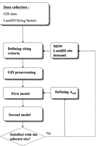
As illustrated in Fig. 1, a typical landfill siting procedure can be implemented as follows. Spatial data and siting factors are collected first. Siting criteria are then determined by the MSW authority taking into consideration the opinions of the general

public and experts. For different local authorities, the consider-ations may be different. The land cost factor will be dominated in an authority with a tight budget but may not for the others. Factors commonly considered will be described later. Obviously inappropriate areas are then excluded based on selected siting factors and criteria after GIS prescreening. Finally, a method to evaluate the suitability of candidate landfill sites is applied to locate the optimal site. The two stage heuristic method proposed in the present study is designed for use in the final step. A size, Asub, which is greater than or equal to the landfill size, is defined

to set the size of subarea. The first model will then find the subarea whose size is smaller than or equal to Asub. After the

subarea is solved, the second model is applied to find the optimal landfill site. The modifications of A_suband siting criteria will be an interactive process if the landfill site is not satisfied.

Several MIP models 共e.g., Wright et al. 1983; Minor and Jacobs 1994; Kao and Lin 1996兲 are available for use with a GIS, but an MIP model generally has difficulties in finding the optimal solution for a large area within an acceptable computational time, especially for a problem considering multiple siting factors. Several heuristic methods have been proposed to overcome this difficulty. Gilbert et al. 共1985兲 applied a heuristic algorithm for solving a grid-based MIP model for a facility siting problem. In each iteration of their approach, multiple objectives were simplified into a single objective with other objectives being set as constraints whose values were restricted to a range not worse than the solution obtained from the previous iteration. The objective applied in each iteration was selected based on decisionmakers’ preferences. This interactive process with decisionmakers’ setting the objective in each iteration is tedious and is not practical for application to a siting problem. Moreover, such a procedure for a large problem may not easily obtain an appropriate solution in a reasonable time because decisionmakers’ choices may not be effective in locating a good solution. Diamond and Wright 共1989兲 proposed an MIP model to solve land allocation problems, with an efficient two-objective method minimizing the cost and using max–min on the other objectives. 1

Assistant Professor, Dept. of Environmental Engineering and Management, Chaoyang Univ. of Technology, Taichung, Taiwan, Republic of China.

2

Professor, Institute of Environmental Engineering, National Chiao Tung Univ., 75 Po-Ai St., Hsinchu, Taiwan 30039, Republic of China 共corresponding author兲. E-mail: jjkao@mail.nctu.edu.tw

Note. Discussion open until March 1, 2006. Separate discussions must be submitted for individual papers. To extend the closing date by one month, a written request must be filed with the ASCE Managing Editor. The manuscript for this paper was submitted for review and possible publication on August 22, 2003; approved on January 26, 2005. This paper is part of the Journal of Computing in Civil Engineering, Vol. 19, No. 4, October 1, 2005. ©ASCE, ISSN 0887-3801/2005/4-369–376/ $25.00.

Several pseudocases, of which the largest is 950 cells, are dem-onstrated in their paper. Recognizing the limitations in solving performance of the model, further research was recommended for exploring improved algorithms or heuristic approaches.

Modern raster- 共or grid-兲 based GIS are frequently used in landfill siting共e.g., Michaels 1988; Kao et al. 1996; Siddiqui et al. 1996兲. For a large grid-based problem, tremendous similar con-straints and variables are required for all grids, and this is an obvious burden that significantly affects solution time. Although heuristic approaches共Ramu and Kennedy 1994; Welch and Salhi 1997兲 are available in many research areas, few are designated for a grid-based problem and, to our knowledge, no existing approach is suitable for solving a grid-based siting problem. An appropriate method should consider multiple objectives and/or factors and solve a problem within an acceptable computational time, and such were the goals of the development of the method present in the present study.

Siting Factors

Multiple decision factors must be analyzed for evaluating the suitability of candidate sites during a landfill siting process 共Zyma 1990; Ramu and Kennedy 1994; Kao et al. 1996兲. Factors such as related regulations/laws 共e.g., distance from a body of water兲, engineering, construction, or budget constraints 共e.g., land slope percent, road accessibility, land cost, etc.兲, and socio-cultural impacts共e.g., distance from a historic/cultural site or a residential area兲 are frequently evaluated in landfill siting. Furthermore, site-specific factors are frequently raised and must

be included due to concerns from the general public or local characteristics. A group decision-making process, which is beyond the scope of this study, is generally applied to determine the set of factors to be evaluated in siting a landfill.

Prescreening

After siting factors are defined, a spatial data processing is generally implemented to screen out unsuitable areas. For instance, Michaels 共1988兲 applied a map-layer overlay approach for a preliminary screen-out of unsuitable areas in a landfill siting problem. The exclusion of obviously unsuitable areas can significantly reduce burden in further analyses. This prescreening can be rapidly accomplished using a GIS. In the present study, GRASS 共1993兲, a public domain raster-based GIS, was used for prescreening. Raster-based data are arranged in cells 共or grids兲 with attribute scores. Each cell represents a land grid and the associated attribute scores express features of the land grid. In this study, all cells are square and of the same size, although varied sizes can also be used. If the area remaining after this prescreening is small, the MIP model previously developed 共Kao and Lin 1996兲 can be applied to find the optimal solution. On the other hand, if the area remaining is large, then the MIP model is impracticable. A heuristic method is therefore proposed as follows.

Heuristic Method

The proposed heuristic method includes two models. The first model is used to find one rectangular subarea with high potential for landfill siting. The level of potentiality is defined as the total score of cell attributes in a subarea. The second model is applied to find the optimal site within the high-potential subarea obtained from the first model. Since the first model is used to find a rectangular area which likely includes the optimal solution and the second model to do the detail optimization, there is no need to use a detailed land grid resolution in the first model. A coarser resolution, with several land grids 共e.g., 2⫻2, 3⫻3,... etc.兲 grouped into a cell, can be applied to save time in solving the first model. The two models are listed and described as follows:

Max

兺

兺

兺

兺

兺

兺

兺

兺

Fig. 1. Proposed prcedure for landfill siting analysis

兺

兺

i=0 M

共ui,j−vi,j兲 = 0 ∀ j 苸 兵0, ... ,N其 共1g兲

兺

兺

兺

兺

兺

兺

j=0 N

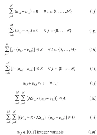
关共Pi,j− R · ASi,j兲 · 共ui,j−vi,j兲兴 艌 0 共1l兲 ui,j苸 关0,1兴 integer variable 共1m兲 where i , j = grid coordinate indices of a land cell for i columns and j rows; M and N = maximum numbers of column and row cells of the siting area, respectively; and CSi,j= lump sum of the total suitability score of cells indexed from 1 to i for the column index and 1 to j for the row index. For convenience in calculation, one column共with i=0兲 and one row 共with j=0兲 of pseudocells, with attribute values set to be zero, are added. Variables ui,jandvi,jare used to determine whether cell i , j is the corner cell of a subarea or not; ui,jis equal to 1 if cell i , j is at the upper-left or lower-right corner andv_i,jis equal to 1 for cell i , j located at the upper right or lower left. Variable ui,j= binary integer variable. It should be noted, as shown in Fig. 2, that only the lower-right corner is exactly in the subarea, and the other three corners are not included. S = limit 共in number of cells兲 for the maximal width 共or height兲 of a subarea; A=maximal size limit 共in number of

cells兲 for a potential subarea; ASi,j= size of the subarea of cells indexed from 1 to i for the column index and 1 to j for the row index; the area of pseudocells are excluded. Therefore, the value of ASi,j is equal to ij, the width multiplied by height. Pi,j= total suitability score of all qualified cells indexed from 1 to i for the column index and 1 to j for the row index. R = lower limit ratio which is the number of qualified cells over the total number of cells in a subarea.

Eq.共1a兲 is the objective function of the first model, it is used to find the selected rectangle subarea whose sum of the total suitability scores is maximum. Eqs. 共1b兲 and 共1c兲 ensure that at most one cell per column or row can be the corner of the desired potential subarea共a rectangular area, as illustrated in Fig. 2兲, and Eq.共1d兲 limits the entire area to two such corners marked by ui,j. Eq. 共1e兲 limits the area to two corners marked byvi,j. There are four corners for a rectangle: two are for ui,j, and the others are for v_i,j. Based on the definition of maximal objective function, the model will be marked in the upper-left or lower-right corners with ui,j= 1, and the upper-right and lower-left ones will be marked withvi,j= 1. Eqs.共1f兲 and 共1g兲 ensure either no corner or pairs of corners共actually, only one pair can be present兲 can be presented in any column or row. With Eqs.共1f兲 and 共1g兲 and the definition of ui,j, binary variablesvi,jneed not be claimed as a binary integer variable, although its values are confined as binary ones. Eqs.共1h兲 and共1i兲 ensure that the width 共height兲 of a subarea is less than the given limits. Since a pair of ui,j= 1 and vi,j= 1 corners must be presented in the same column or row, the difference of the position indices of nonzero ui,jandvi,jis the height or width of the desired subarea. Eq.共1j兲 ensures a cell can be at most one of

Fig. 2. Subarea and its four corners, as defined and used in first

model of proposed two stage method

Fig. 3. Sample共a兲 suitability and 共b兲 accumulative score map layers

Fig. 4. Illustration of how to calculate area/score of subarea

four corners. Eq.共1k兲 limits the size 共in number of cells兲 of the desired subarea. Because some cells are excluded during the prescreening and too many exclusions will make the cells in the subarea too sparse, Eq.共1l兲 is added to ensure the located subarea must have at least a specified ratio共R兲 of qualified cells.

Fig. 3 illustrates the relationship between a suitability map layer and the accumulative score map layer. Each number in a cell of the accumulative map layer represents the accumulated scores of the cells whose index numbers共i, j兲 are less than or equal to 共top/left兲 the accumulated one. As shown in Fig. 4, the total score of the indicated subarea can be computed based on four subareas. The total score of the subarea is equal to the sum of subareas C1 and C4 minus subareas C2 and C3. The accumulated score for a subarea is equal to the sum of the scores of the upper-left共C1兲 and lower-right共C4兲 corner cells minus those of upper-right 共C2兲 and lower-left 共C3兲 cells. Please note that only the lower-left corner cell is located inside the subarea and the three other corner cells are outside but adjacent to the subarea.

After a subarea with high potentiality is obtained from the first model, the second model is applied to find the optimal site. This model is modified from a model developed in our previous study 共Kao and Lin 1996兲. It ensures that the cells of the selected site are tightly integrated 共compact兲 and not discrete or discontinuous. Detailed discussions regarding compactness and our previous model can be seen in Kao and Lin共1996兲. To ensure that each cell in the subarea has adjacent cells, a pseudorow of cells共for j=n+1兲 on the bottom and a pseudocolumn 共for i=0兲 of cells on the left are added before setting up the model

Max

兺

兺

j=n+1

C_i,j· s_i,j 共2a兲

Subject to

2si,j− si,j−1− si+1,j+ ti,j艌 0

∀i 苸 兵0, ... ,m其; ∀ j 苸 兵1, ... ,n + 1其 共2b兲

兺

兺

兺

兺

where Ci,j= attribute score of cell i , j; Si,j= integer variable; if cell i , j is part of the landfill site, then si,j is equal to 1; m and n = numbers of columns and rows of cells in the high potential subarea; Ar= required size 共in numbers of cells兲 of the desired site; ti,j= pseudovariable used for computing the perimeter共in numbers of cell sides兲 of the desired site, the sum of

ti,j= half the total perimeter of the desired site; and P = limit for half the perimeter of the desired site.

Eq. 共2a兲 is the objective function of the model, maximizing the total attribute score of the selected site. Eq. 共2b兲 is used to determine the valid side in the perimeter of the desired site. Eq. 共2c兲 limits the perimeter and therefore assures the compact-ness of the desired site. Eq. 共2d兲 limits the size of the desired site. In comparison with other MIP models, as listed in Table 1, the second model 共Kao and Lin 1996兲 is with less variables and constraints which will save the solving time. The numbers of variables and constraints were calculated for each cell in establishing the model.

Before applying the first model, a limitation on the size of the subarea, A, should be set. If A is set to the size of the entire siting area, then there is no need to apply the first model. On the other hand, if A was set to Ar, the size of the desired site, there is no need to apply the second model. If A is set too large, a solution takes too much computational time. If A is set too small, little computational time will be needed to solve the second model, but the probability of locating the true optimal site will be reduced. A siting process may start with a small value of A, requiring a short computational time; the value may be increased if the solution is not likely to be close to the true optimal site.

This heuristic method saves solving time because the model size is significantly reduced. Assuming the numbers of required variables and constraints for each land cell in a model are denoted by V and C, respectively, and the model is applied to a case with N cells, variables and constraints not directly related to each cell can be neglected because they are usually trivial when compared with those required for cells. In such a case, the total numbers of variables and constraints would be approximately VN and CN, respectively. For example, if a model requires three variables and two constraints per cell, then for a case of 10,000 cells, the model needs at least 30,000 variables and 20,000 constraints. However, for the first model of the proposed method with the resolution of 2⫻2, only about 5,000 variables and 2,500 constraints are required, while two共V=2兲 variables and one 共C=1兲 constraint are required for each grouped cell. Further reduction can be observed if a coarser resolution is used. Table 1 lists the numbers of constraints/variables required for each cell for three different MIP siting models. Even for the model with the least constraints/variables共Kao and Lin 1996兲, some 20,000 variables and 10,000 constraints are required for a case of 10,000 cells 共V=2 and C=1兲. Required solving time for the second model in the proposed method is trivial when compared with that for solving the first model because the number of cells remaining in stage 2 is much less than that in stage 1. Siting problems are NP hard problems and reduction of the number of constraints/ variables by half will save more than half of the time required to solve the original model.

In the following section, a case study is described to demon-strate the effectiveness of the proposed method.

Case Study

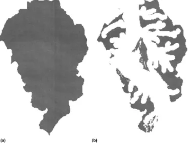
The proposed method was applied to a landfill siting problem in Shihu County in central Taiwan, Republic of China. Fig. 5共a兲 shows the entire siting area, with an area of about 41 km2_{. At a}

resolution of 40 m⫻40 m, the area can be divided into about 25,700 cells. A preliminary screening procedure was applied to exclude obviously inappropriate areas before the two stage method was utilized. Various rules for landfill siting were adopted

Table 1. Comparison of Three Mixed Integer Programming Models Based on Required Numbers of Variables and Constraints for Each Cella Model

Number of integer

共noninteger兲 variables Number ofconstraints

Minor and Jacobs共1994兲 3共0兲 8

Wright et al.共1983兲 5共0兲 2

Kao and Lin共1996兲 1共1兲 1

a

Kao and Lin共1996兲.

to define siting criteria. According to the criteria, those cells not satisfying any of the criteria were excluded by map-layer analysis functions provided by GRASS共1993兲. Subsequently, the proposed two-stage models were applied to obtain a high potential subarea and the optimal site in the subarea, respectively.

Siting Criteria

Similar to the criteria used in former research共Lin 1985; Lin and Kao 1999兲, environmental, socio-culture, and engineering-economic siting criteria were considered herein, as described below.

Environmental Criteria

1. Surface water: a landfill should be placed away from rivers, lakes, or other surface water bodies. A buffer zone of 180 m is used for this example.

2. Ground water and drinking water resources: a landfill should not be placed in the proximity of ground water or drinking water resources protection areas.

3. Floodplain: a landfill should not be placed within a flood-plain, to reduce the risk of overland drainage pollution. Socio-Cultural Criteria

1. Urban development: a landfill should not be placed on a site close to a residential or urban area to avoid negative impact on future development, and to protect the general public from possible risks caused by environmental hazards from a landfill site. A buffer zone of 150 m between a landfill site and a residential or urban area was used for this example. 2. Historical or cultural sites: a landfill site should not be placed

on a site close to historic/cultural/scenic sites. A buffer zone of 500 m from such sites was used.

Engineering-Economic Issues

1. Fault zones: fault zones can lead to instability in construc-tion. Siting must be done at distance from existing fault zones. Here, the distance is set to 80 m.

2. Land slope: an area with a large land slope may be unstable, thereby increasing construction and maintenance difficulty.

Areas with a land slope in excess of 40% were ruled out in this case study.

3. Land cost: there is no need to use a site with a high land cost for placing a landfill. In this work, land cells costing more than 50% of the highest price were ruled out.

4. Road network accessibility: a landfill should not be placed too far away from the transportation system, so that MSW

Fig. 5. Entire siting area and accepted subareas:共a兲 the entire siting

area and共b兲 the accepted sub-areas for further analysess

Fig. 6. Suitability scores for:共a兲 land slope percent; 共b兲 land cost;

and共c兲 road network accessibility

Fig. 7. Total scores for acceptable cells in siting area

collection and transportation costs can be reduced. In this example, the landfill had to be placed within 1 km of existing roads.

The entire siting area was prescreened using GRASS 共1993兲 and 9,055 cells, distributed in 266 columns and 190 rows, were left after this prescreening, as illustrated in Fig. 5共b兲.

Siting Factors

Three siting factors 共land slope, land cost and road network accessibility兲 were selected for the following analyses. Depending on the value of each factor of a cell, a score is assigned to express its appropriateness for becoming a portion of a landfill site. Suitability scores for the three siting factors of each cell were assigned according to the figures in Fig. 6, modified from Lin and Kao 共1999兲. For use with the heuristic model, a higher score implies a higher suitability. These factors are briefly described below.

1. Land slope percent共S兲: a land slope percent between 8 and 12% is regarded as an appropriate slope for constructing a landfill. Too steep a slope would make the landfill difficult to construct and maintain, and too flat a slope would make the runoff difficult to drain. Fig. 6共a兲 shows the suitability scores assigned for various land slopes.

2. Land cost共C兲: only cells with a unit land cost less than half of the maximum are assigned scores. The higher the land cost, the lower the suitability score, as illustrated in Fig. 6共b兲. 3. Road network accessibility 共R兲: placing a landfill site far away from the existing road network would increase the cost for constructing the necessary connection road. Therefore, cells closer to an existing road network are assigned higher scores, as shown in Fig. 6共c兲.

Each cell surviving the prescreening is assigned suitability scores for the factors and the total score of a cell is determined by summing each factor score multiplied by its associated weight. As used in Lin and Kao共1999兲, weights for the three factors were set to 3.8 共land slope兲, 3.2 共land cost兲, and 3.4 共road network accessibility兲, respectively. Fig. 7 shows the total suitability score map. Blank cells indicate excluded area, and brighter cells indicate higher scores.

Heuristic Analysis

After the suitability score map was prepared, the proposed heuristic models were applied. Map layers with varied resolutions were analyzed using the first model. A lower resolution generates fewer cells, thereby the computational time can be significantly shortened; in contrast, a higher resolution requires more computational time to solve the models. A low resolution for the first model and a high resolution for the second model are recommended. The original map layer was composed of cells with a resolution of 40 m⫻40 m and was transformed into three resolutions of 80 m⫻80 m 共12,672 cells for the entire siting area兲, 120 m⫻120 m 共5,632 cells兲, and 160 m⫻160 m 共3,168 cells兲 for the application of the first model for finding a high potential subarea. The score for each cell at various resolutions is determined by the average of scores of the original 40 m⫻40 m cells within it.

The landfill currently operating in Shihu County is about

Table 2. Scenarios for Case Studied Resolution

Landfill area: 2.56 ha Subarea number of cells

Landfill area: 5.76 ha Subarea number of cells 80 m⫻80 m 4共16兲a 6共24兲 9共36兲 9共36兲 12共48兲 16共64兲 120 m⫻120 m 2共18兲 4共36兲 9共81兲 4共36兲 9共81兲 12共108兲 160 m⫻160 m 1共16兲 4共64兲 9共144兲 4共64兲 9共144兲 16共256兲 a

The number of the cells of a subarea in the corresponding resolution where the number in the parentheses is the number cells in the original resolution共40 m⫻40 m兲.

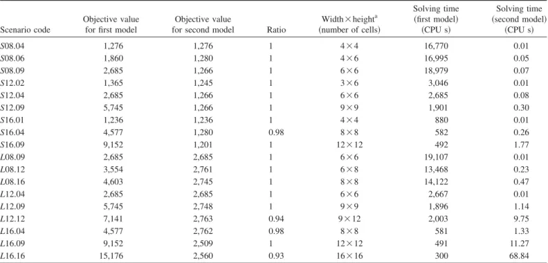
Table 3. Results Obtained for Varied Scenarios

Scenario code

Objective value for first model

Objective value

for second model Ratio

Width⫻heighta 共number of cells兲 Solving time 共first model兲 共CPU s兲 Solving time 共second model兲 共CPU s兲 S08.04 1,276 1,276 1 4⫻4 16,770 0.01 S08.06 1,860 1,280 1 4⫻6 16,995 0.05 S08.09 2,685 1,266 1 6⫻6 18,979 0.07 S12.02 1,365 1,245 1 3⫻6 3,046 0.01 S12.04 2,685 1,266 1 6⫻6 2,685 0.08 S12.09 5,745 1,266 1 9⫻9 1,901 0.30 S16.01 1,236 1,236 1 4⫻4 880 0.01 S16.04 4,577 1,280 0.98 8⫻8 582 0.26 S16.09 9,152 1,201 1 12⫻12 492 1.77 L08.09 2,685 2,685 1 6⫻6 19,107 0.01 L08.12 3,554 2,761 1 6⫻8 13,468 0.23 L08.16 4,603 2,745 1 8⫻8 14,122 0.47 L12.04 2,685 2,685 1 6⫻6 2,667 0.01 L12.09 5,745 2,748 1 9⫻9 1,896 1.14 L12.12 7,141 2,763 0.94 9⫻12 2,003 9.75 L16.04 4,577 2,762 0.98 8⫻8 581 1.33 L16.09 9,152 2,509 1 12⫻12 491 11.27 L16.16 15,176 2,560 0.93 16⫻16 300 68.84 a

In the original resolution, 40 m⫻40 m.

3.9 ha in area and will be closed soon. It has been in use for more than 15 years. The desired new landfill size is 2.56 or 5.76 ha. Various size limits for the potential subarea were analyzed. Table 2 lists 18 different scenarios with various potential subarea size limits, landfill sizes, and resolutions. There are nine scenarios for both desired landfill sizes. For instance, the first row of last column of 2.56 ha is 9共36兲, it means the size of subarea is set to nine cells 共A in first model兲 in the modified resolution 共80 m⫻80 m兲 or 36 cells in the original resolution 共40 m⫻40 m兲, note that the landfill size is only 2.56 ha, four modified cells or 16 original cells, which will be solved after

applying the second model. Except for the one exactly equal to the desired landfill size, the ratio of remaining cells after prescreening in the subarea was set to 0.75. For convenience, to distinguish the scenarios in the following description, each scenario is named using S共L兲RR.NN, where S or L indicates a scenario for a small共2.56 ha兲 or large 共5.76 ha兲 desired landfill size, respectively; RR indicates the resolution of the scenario, 08共80 m⫻80 m兲, 12 共120 m⫻120 m兲 and 16 共160 m⫻160 m兲; and NN indicates the number of cells of the desired subarea. For instance, L16.09 refers the scenario with a 160 m⫻160 m resolution and a subarea with at most nine cells. Models for these scenarios were solved by CPLEX共ILOG Inc. 1997兲 on a Pentium Pro PC with 128 MB RAM.

Results

Table 3 lists the results for all scenarios, including the objective value of the first model, the objective value of the second model, the actual ratio of qualified cells in the subarea, the scale of the subarea, and the computational time to solution for the first and second models. The objective values of the two models are different because the first objective value is the total scores of the subarea, and the second is of the landfill site. In the table, “width⫻height” indicates the size of the obtained subarea in the original resolution of 40 m⫻40 m. The solving time for the first model decreases when the resolution of map layer decreases because a low resolution has fewer cells, and vice versa. For scenarios S共L兲08.x, average computational time is about 16,574 s, a figure much greater than the 2,136 s for S共L兲12.x and 554 s for S共L兲16.x. Compared with the computational time spent solving the first model, solving time for the second model is insignificant.

The average total attribute score of the selected site in S08. x is

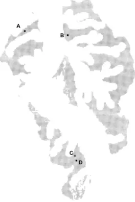
Fig. 8. Shape of selected sites in all scenarios

Fig. 9. Locations of selected sites

1,274 and 2,730 for L08. x, 1,259 for S12. x, and 2,732 for L12. x, and 1,239 for S16. x and 2,610 for L16. x. Attribute scores for several small cells in a high resolution are averaged to yield the score of a new large cell in a low resolution. Small cells with “excellent” scores can be averaged and reduced to a “good” value if they are surrounded by several cells with marginal “qualified” scores. Therefore, a higher average total attribute score for the selected site likely occurs at a higher resolution. However, with a higher resolution, solution time is often unacceptable for a real case. We suggest that the analyst should start with a low resolu-tion that can be solved quickly and then, based on the quality of the selected site, decide whether to apply the proposed method further for a higher resolution. The score of the true optimal solution for the desired landfill size of 2.56 ha is 1,301, and scores of most solutions 共Sx.x兲 obtained from the proposed heuristic method are close to it. The optimal solution for Lx . x is 2,869 and takes a long CPU time of 59,423 s: significantly longer than that required for applying the proposed heuristic method. Most solutions obtained by applying the proposed heuristic method for Lx . x cases are close to the optimal solution. In all scenarios, varied size limits of the potential subarea were tested, including one equal to the desired landfill size. Most heuristic solutions are compatible with the optimal solutions except in a very few scenarios. Although “equal size” solutions are not good, a large subarea did not always promise a site with a better total score in the second model. The reason is that the score of final solutions varies with the distribution of cells with good attribute values. If many cells with good scores are grouped together in a few subareas of the siting area, a large size limit may be desirable. However, if good cells are sparsely distributed, a large limit may not always give a good result, as demonstrated in this case. The shape and location of each selected site are presented in Figs. 8 and 9, respectively. All selected sites are compact enough to be placed at a landfill. Most of the sites are located close to point B, but a few other sites are found in other locations close to A, C, and D.

Conclusions

The two-stage heuristic approach proposed in this study can be applied to resolve a raster-based landfill siting problem. The approach can facilitate siting analysis and reduce solution time to locate an appropriate site from a large area. Solution time increases with the number of cells, so setting a suitable resolution is important. A low resolution is strongly recommended for the first application because a solution can be quickly obtained. Then, according to the quality of the result, the analyst can decide whether to spend more computational time to solve the problem further at a higher resolution. The size limit of the potential subarea to be located is not the dominating factor for the required solving time; a large size limit can produce good results if good cells are grouped together in the siting area. However, as demon-strated, a large size limit may not locate a better solution in comparison with a small size limit when good cells are sparsely distributed. If the quality of the solution is not acceptable, various size limits may be applied to explore a better solution. In comparison with a MIP model for solving the landfill siting problem, the maximal number of possible solutions is 2X_, increasing exponentially with the number共X兲 of total cells, and solution time would become impractical. The first model proposed in this study selects two cells from all cells, which are

the upper-left and lower-right corners of the subarea. Hence, the exact number of combinations in the solution space is _XC₂ which is fewer than X2 _{and significantly smaller than 2}X_, especially for a large X. With the proposed approach, a large siting problem that cannot be solved practically using a MIP model can now be resolved.

The method is currently applicable for a raster-based problem. It would be useful to develop a similar approach for vector-based data. Ongoing research has been implemented to develop such a vector-based approach. Finally, although the heuristic approach was demonstrated for a landfill siting problem, it is also applicable for other land siting problems for facilities such as incinerators, recycling facilities, and transfer stations.

Acknowledgment

The writers would like to thank the National Science Council, Taiwan, for providing partial financial support of this work under Grant No. NSC-91-2211-E324-004.

References

Diamond, J. T., and Wright, J. R. 共1989兲. “Efficient land allocation.” J. Urban Plann. Dev., 115共2兲, 81–96.

Gilbert, K. C., Holmes, D. D., and Rosenthal, R. E. 共1985兲. “A multi-objective discrete optimization model for land allocation.” Manage. Sci., 31共12兲, 1509–1523.

Goodchild, M. F., Parks, B. O., and Steyaert, L. T.共1993兲. Environmental modeling with GIS, Oxford University Press, New York.

GRASS4.1 user’s reference manual.共1993兲. United States Army Corps of Engineers, Construction Engineering Research Laboratory, Champaign, Ill.

ILOG Inc. 共1997兲. Using the CPLEX callable library, Incline Villiage, Nev.

Kao, J. J., Chen, W. Y., Lin, H. Y., and Guo, S.-J. 共1996兲. “Network expert geographic information system for landfill siting.” J. Comput. Civ. Eng., 10共4兲, 307–317.

Kao, J. J., and Lin, H. Y.共1996兲. “Multifactor spatial analysis for landfill siting.” J. Environ. Eng., 122共10兲, 902–908.

Lin, H. Y., and Kao, J. J. 共1999兲. “Enhanced spatial model for landfill siting analysis.” J. Environ. Eng., 125共9兲, 845–851.

Lin, S. J.共1985兲. The analysis of criteria of waste processing facilities and landfill siting, Economics and Construction Committee, Taiwan Provincial Government, Taiwan共in Chinese兲.

Lindquist, R. C.共1991兲. “Illinois cleans up: Using GIS for landfill siting.” Geo. Info. Systems, February, 30–35.

Michaels, M. 共1988兲. “GIS expected to make landfill siting easier.” World Wastes, December, 32–36.

Minor, S. D., and Jacobs, T. L. 共1994兲. “Optimal land allocation for solid- and hazardous-waste landfill siting.” J. Environ. Eng., 120共5兲, 1095–1108.

Ramu, N. V., and Kennedy, W. J.共1994兲. “Heuristic algorithm to locate solid-waste disposal site.” J. Urban Plann. Dev., 120共1兲, 14–21. Siddiqui, M. Z., Everett, J. W., and Vieux, B. E.共1996兲. “Landfill siting

using geographic information systems: A demonstration.” J. Environ. Eng., 122共6兲, 515–523.

Welch, S. B., and Salhi, S. 共1997兲. “The obnoxious p facility network location problem with facility interaction.” Eur. J. Oper. Res., 102, 302–319.

Wright, J., ReVelle, C., and Cohon, J.共1983兲. “A multiobjective integer programming model for the land acquisition problem.” Region. Sci. Urban Econ., 13, 31–53.

Zyma, R.共1990兲. “Siting considerations for resource recovery facilities.” Public Works, September, 84–86.