具I/O裝置的弱即時性系統之省電排程演算法

全文

(1)國立高雄大學資訊工程學系碩士論文. 具 I/O 裝置的弱即時性系統之省電排程演算法 Energy-Aware Scheduling for Weakly-Hard Real-Time System with I/O Device. 研究生：陳再興撰指導教授：郭錦福. 中華民國一百零一年七月.

(2) 具 I/O 裝置的弱即時性系統之省電排程演算法指導教授：郭錦福博士國立高雄大學資訊工程學系. 學生：陳再興國立高雄大學資訊工程學系. 摘要. 在嵌入式系統當中，除了處理器之外，還具有一些周邊裝置（例如記憶體，快閃記憶體，無線網路介面等）這些裝置都會消耗電量。動態電源管理技術（DPM）常以超時機制，在特定的時間範圍，將裝置切換成閒置狀態，以最小化周邊裝置的能源損耗。在某些即時系統中要求的是，必須滿足某個決定性的 QOS 等級，而非 100%都滿足，亦非達到某個 QOS 機率。所以該系統須要支援靜態且滿足最小限度的 QOS 等級。正如同 (m,k) 限制，連續 k 個工作中至少要有 m 個必須在時限之前完成。我們提出以搜尋樹為基礎的省電排程演算法，來解決具有 IO 裝置的弱即時系統的排程問題。針對提出的演算法，我們會進行分析及研究，並以一系列的模擬實驗，驗證分析的結果，以及展現演算法的各種效能。關鍵字：弱即時性系統、I/O 裝置、省電排程、搜尋樹、(m,k) 模型.

(3) Energy-Aware Scheduling for Weakly-Hard Real-Time System with I/O Device Advisor: Dr. Chin-Fu Kuo Department of Computer Science and Information Engineering National University of Kaohsiung. Student: Tsai-Hsiung Chen Department of Computer Science and Information Engineering National University of Kaohsiung. ABSTRACT. In addition to processors, embedded systems also have some peripheral devices (such as: memory, flash memory, wireless interface). These devices will also consume energy. Dynamic power management (DPM) technology is often used to minimize the energy consumption of peripheral devices with the timeout mechanism in which the device is switched to the idle state for a specific time interval. Because the requirement of some systems is to support deterministic QoS for real-time systems, rather than 100% guarantees or the probabilistic QoS, the system must support the statistical and the lowest limit of QoS, such as (m, k) constraints, which require that at least m out of any k consecutive jobs of a task meet their deadlines. We proposed search-tree-based energy-efficient algorithm to solve the scheduling problem of weakly-hard real-time system with an I/O device. An analytic study on the proposed algorithms is presented, and a series of simulation experiments are conducted to verify the analytic results and to show the capability of the proposed algorithm. Keywords: Weakly-hard real-time systems, I/O device, Energy aware scheduling, Search tree, (m, k) model..

(4) Contents 1. Introduction. 4. 2. System Model. 6. 3. Motivation Example. 8. 4. Energy-Efficient Algorithm for Weakly-Hard Real-Time System With I/O Device 12. 5. 6. 4.1. Basic Search-Tree-based Energy-Efficient Algorithm . . . . . . . . . . . . .. 12. 4.2. Advance Search-Tree-based Energy-Efficient Algorithm . . . . . . . . . . .. 17. Performance Evaluation. 23. 5.1. Experiment Setup and Performance Metrics . . . . . . . . . . . . . . . . . .. 23. 5.2. Experimental Results . . . . . . . . . . . . . . . . . . . . . . . . . . . . . .. 24. Conclusion. 31. Bibliography. 31. 1.

(5) List of Figures 3.1. Motivation Example. . . . . . . . . . . . . . . . . . . . . . . . . . . . . . .. 9. 4.1. The parent node and the oldest child node. . . . . . . . . . . . . . . . . . . .. 13. 4.2. Append the second child node. . . . . . . . . . . . . . . . . . . . . . . . . .. 13. 4.3. The coordinate of the search tree example. . . . . . . . . . . . . . . . . . . .. 14. 4.4. The BSTEE search tree of depth 1. . . . . . . . . . . . . . . . . . . . . . . .. 16. 4.5. The BSTEE search tree of depth 2. . . . . . . . . . . . . . . . . . . . . . . .. 17. 4.6. The BSTEE search tree of depth 3. . . . . . . . . . . . . . . . . . . . . . . .. 18. 4.7. The BSTEE completed schedule tree. . . . . . . . . . . . . . . . . . . . . .. 20. 4.8. The ASTEE search tree of depth 1. . . . . . . . . . . . . . . . . . . . . . . .. 21. 4.9. The ASTEE search tree of depth 2. . . . . . . . . . . . . . . . . . . . . . . .. 21. 4.10 The ASTEE search tree of depth 3. . . . . . . . . . . . . . . . . . . . . . . .. 21. 4.11 The ASTEE completed schedule tree. . . . . . . . . . . . . . . . . . . . . .. 22. 5.1. The normalized energy consumption when (m,k) = (3,10) . . . . . . . . . . .. 25. 5.2. The normalized energy consumption when (m,k) = (6,10) . . . . . . . . . . .. 26. 5.3. The normalized energy consumption when (m,k) = (9,10) . . . . . . . . . . .. 27. 5.4. The number of generated nodes when (m,k) = (3,10) . . . . . . . . . . . . .. 27. 5.5. The number of generated nodes when (m,k) = (6,10) . . . . . . . . . . . . .. 28. 5.6. The number of generated nodes when (m,k) = (9,10) . . . . . . . . . . . . .. 28. 5.7. The number of physicaly required nodes when (m,k) = (3,10) . . . . . . . . .. 29. 5.8. The number of physically required nodes when (m,k) = (6,10) . . . . . . . .. 29. 5.9. The number of physically required nodes when (m,k) = (9,10) . . . . . . . .. 30. 2.

(6) List of Tables 3.1. Task parameters of an example task set . . . . . . . . . . . . . . . . . . . . .. 8. 3.2. Power consumption parameters of an example device . . . . . . . . . . . . .. 8. 3.3. Task parameters of the task set with (m, k)-constraints . . . . . . . . . . . .. 10. 3.4. Job list ordered by arrival time . . . . . . . . . . . . . . . . . . . . . . . . .. 10. 3.5. Job list after partition . . . . . . . . . . . . . . . . . . . . . . . . . . . . . .. 11. 4.1. Definitions of Notations . . . . . . . . . . . . . . . . . . . . . . . . . . . . .. 16. 5.1. Power consumption parameters of experiment . . . . . . . . . . . . . . . . .. 24. 3.

(7) Chapter 1 Introduction Power-saving technology has been a very important issue, especially in embedded systems or in a variety of battery-powered devices. Power on behalf of life, to save more power consumption can extend longer system lifetime. Power-saving technologies can be classified to two levels: hardware (static) and software (dynamic). Static power management (SPM) techniques, such as synthesis and compilation for low power, are applied at design time (off-line)[1]. Dynamic power management (DPM) refers to collect and analyze system information at run time, such like current system loading or remaining energy, and then adjust the system works in order to achieve energy saving [5]. DPM is more flexible to be applied into different hardware platforms. Real-time application such as VoIP and video stream may use I/O resources during run time and may have soft deadlines. Much relevant research literature of DPM has been proposed, one of the most popular and effective technology is dynamic voltage scaling (DVS), and much research have been proposed, e.g., [2, 7, 15]. The rationale behind DVS is to reduce the speed and voltage of the processor to achieve energy saving if possible. The energy consumption of a processor is quadratically proportional to its operating voltage [13]. However, slower processor speed means that the execution time of tasks will be longer. In modern systems, processors and I/O subsystems are two major energy consumers. If I/O resources is included into the system model, then serval important issues need to be solved: 1. Longer I/O blocking time may lead other tasks missing their deadlines. 2. I/O resources have multiple power states and their own context switch overhead. 3. Longer I/O resources allocation time may lead system energy increased. (In other words, the added energy consumption by resources may be larger than the reduced energy consumptions from the processor).. 4.

(8) From the above issues, we can observe that a DVS mechanism may not be efficient to deal with a system with I/O resources. Unlike hard real-time systems, real-time application such as VoIP and video stream, may use I/O resources during run time and may have soft deadlines, where tasks which do not finish by their deadlines can still be completed with a reduced value[9], or they can simply be dropped with-out compromising the desired quality of service (QoS)[8]. The QoS level refers to several related aspects of telephony and computer networks that allow the transport of traffic with special requirements. To provide a deterministic QoS to a real-time system, [3]presented (m, k) model, out of k consecutive task instance any m instance must meet their respective deadlines, where m and k are two positive integers with m ≤ k . If m = k, the application is a hard real-time application. To guarantee the(m, k)-constraints, [12] proposed a strategy to partition the jobs into mandatory and optional jobs. The mandatory jobs are the jobs that must meet their deadlines in order to satisfy the (m, k)-constraints, while the optional jobs can be executed to further improve the quality of the service or simply be dropped to save the computing resources. The partitioning problem is NP-hard. [11] This paper aims to find out the jobs execution orders with a minimal energy consumption for a weakly-hard real-time system with the (m, k) constrains based on three kinds of heuristic techniques: deeply red pattern (DR)[8], evenly distributed pattern (ED)[12] and reversed evenly distributed pattern (RED)[10]. We developed a energy-efficient algorithm for the scheduling problem and then analyze the output to find out the effect to the job list by the different (m, k) model heuristic techniques. The rest of this paper is as follows: chapter 2 defines the system model and give the concepts of DR, ED, and RED. chapter 3 proposes a motivational example for our proposed algorithm. chapter 4 presents an search-tree based energy-efficient algorithm for a weakly-hard real-time system with an I/O device. In chapter 5, a series of simulation experiments are done for evaluating the performance of the proposed algorithm. chapter 6 is the conclusion.. 5.

(9) Chapter 2 System Model We focus on the system with a single non-DVS processor. In the system, there are a set of N periodic and independent tasks Γ = {T0 , T1 , ..., TN −1 }. Let Ti,j is the j-th job instance of task Ti . Each task Ti is associated with five parameters : (Pi , Di , Ci , (mi , ki )). Pi is the period of the task and Ci is the worst-case execution time (WCET). Di is the relative deadline (Pi ≤ Di ), and we assume that the deadline of each task is equal to it’s period. mi and ki (0 < mi ≤ ki ) define the (m, k) constraints for Ti . The hyperperiod H of a task set is calculated based on the least common multiple (LCM) of all tasks’ periods and (m, k) patterns of tasks, H = LCM {Pi ∗ ki }, where i = 0, 1, ..., N − 1. Each task Ti will access one I/O device A. We assume that the device is used in a nonpreemptible fashion, such as a printer. The processor and the device have two states : active andsleep, Pa denotes the power consumed per unit time when the device(or processor) is on the active state and Ps is the power consumed per unit time when the device(or processor) is on the sleep state. Pwu is the power consumed per unit time when the device is switched to the active state from the sleep state and Psd is the power consumed per unit time when the device is switched to the sleep state from the active state. Twu is the device transition time from the sleep state to the active state and Tsd is the transition time from the active state to the sleep state. Then we have to consider how to meet the (m, k)-constraints. Much works has been conducted in scheduling (m, k) model. A common approach is to statically partition the jobs of each task into two groups: mandatory and optional, and that all mandatory jobs meet their deadline can ensure (m, k)-constraints. Then we will introduce three kinds of heuristic techniques. [Deeply-Red Pattern] This pattern was proposed by [8]. The j-th job Ti,j of a task Ti is. 6.

(10) mandatory if j mod ki < mi , j = 0, 1, 2, ...,. (2.1). and otherwise is optional. [Evenly-Distributed Pattern] The second static partitioning policy was proposed by [12]. Job Ti,j is mandatory if j = ⌊⌈j ×. ki mi ⌉× ⌋, j = 0, 1, 2, ..., ki mi. (2.2). and otherwise is optional. [Reverse-Evenly-Distributed Pattern] The third pattern was proposed by [10]. This patter is a reverse of Evenly-Distributed Pattern. Job Ti,j is optional if j = ⌊⌈. j × (ki − mi ) ki ⌉× ⌋, j = 0, 1, 2, ..., ki (ki − mi ). (2.3). and otherwise it is mandatory. Using these partition polices, all jobs of each task can be marked to be a mandatory or optional job.. 7.

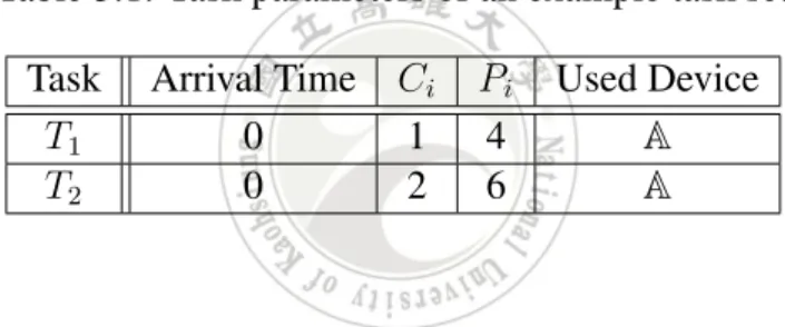
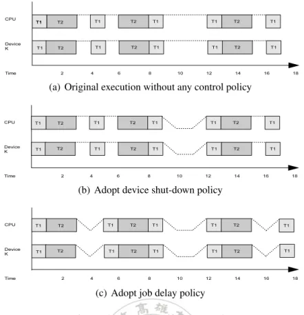
(11) Chapter 3 Motivation Example In this chapter we consider an example to present our motivation. The parameters of task set are shown in Table 3.1, T1 and T2 are both arrival at time 0 and use the same I/O device A. The period and the execution time of T1 (/T2 ) are 4(/6) and 1(/2), respectively. The power consumption parameters of device A are shown in Table 3.2 [14]. Table 3.1: Task parameters of an example task set Task T1 T2. Arrival Time 0 0. Ci 1 2. Pi 4 6. Used Device A A. Table 3.2: Power consumption parameters of an example device Device A Processor. Pa 3 6. Ps 1 2. Psd =Pwu 2 4. Tsd =Twu 1 1. Figure 3.1(a) shows that no energy-efficient control policy is applied to the system. The processor and the device always keep on the active state. At t = 17, the total energy consumption from t = 0 to t = 17 is equal to ((Pa of the processor )*(the active time of the processor)) + ((Pa of the device)*(the active time of the device)) = (6*17) + (3*17) = 153. We can observe that the system is idle in the following intervals: (1)from t =3 to t = 4, (2)from t = 5 to t =6, (3)from t = 9 to t = 12, and (4)from t = 15 to t = 16. If an idle time interval is larger than the break-even time [4], then we can shut down the processor and the. 8.

(12) (a) Original execution without any control policy. (b) Adopt device shut-down policy. (c) Adopt job delay policy. Figure 3.1: Motivation Example I/O device to reduce the energy consumption. Figure 3.1(b) shows that the processor and the device A are shut down at t = 9, and then is switched to the active state at t = 11 for ready to work. So the total active time of the processor is 14. During the interval from t = 9 to t = 12, the processor is switched to the sleep state at t = 9 then is switched to the active state at t = 11. The total energy consumptions of the processor from t = 9 to t = 12 is ((Psd of the processor) * (Tsd of the processor)) + ((Ps of the processor) * (sleep time)) + ((Pwu of the processor) * (Twu of the processor))= 4*1 + 2*2 + 4*1 = 12. The total energy consumptions of the the processor from t = 0 to t = 17 is ((Pa of the processor) * (active time)) + 12 = 6*14 + 12 = 96. We can derive the total energy consumptions of the device with the similar way : ((Pa of device) * (active time)) + 6 = 48. Finally, we get the total energy of the system (including the processor and the device) is 96 + 48 = 144. Figure 3.1(c) shows that the execution of the second job of task T1 is not started until t = 5. Such execution delay does not cause any deadline missing and generates an idle interval from t = 3 to t = 5. Therefore, the processor and the device can be shut down in the time interval. Besides, the execution of the third job instance of task T1 can be delayed to t = 17 and then the finished time is at t = 18. The energy consumptions of the processor from the interval from t=0 to t =18 is equal to 94(=6* 3 + 4*1 + 4*1 + 6*4 + 4*1 + 2*2 + 4*1 + 6*3 + 4*1 + 4*1 + 6*1).. 9.

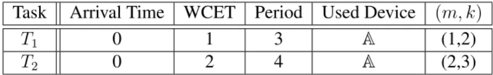
(13) We can derive the total energy consumption 47 of the device with the similar way. Finally, the total energy consumption of the system is 141(=94 + 47). Although the whole system is active in the time interval from t = 17 to t = 18, the total energy consumption of the system becomes smaller. Next, we will consider a task set with (m, k)- constraints as shown at Table 3.3. The control policies, i.e., the device shut-down policy and the job delay policy, will be applied to the (m, k) task set. Table 3.3: Task parameters of the task set with (m, k)-constraints Task T1 T2. Arrival Time 0 0. WCET 1 2. Period 3 4. Used Device A A. (m, k) (1,2) (2,3). We generate a job list for the task set in the hyper-period 12 of the tasks and then adopt the Deeply-Red Partition policy to partition these jobs as mandatory and optional jobs, then sort jobs by arrival time, as shown in Table 3.4. The notations “M” and “O” means a mandatory job and an optional job, respectively. Table 3.4: Job list ordered by arrival time Job Arrival Time WCET Task Instances Use Device Type. job1 0 1 T1,1 A M. job2 0 2 T2,1 A M. job3 3 1 T1,2 A O. job4 4 2 T2,2 A M. job5 6 1 T1,3 A M. job6 8 2 T2,3 A O. job7 9 1 T1,4 A O. All mandatory jobs meeting their deadlines can ensure that (m, k)-constraints are guaranteed. Besides, in order to minimize energy consumptions, optional jobs are ignored directly and not executed. Finally we get a new job list, as shown in Table 3.5. In the next chapter, we will apply the proposed basic search-tree-based energy-efficient algorithm (OSTEE) and advance search-tree-based energy-efficient algorithm (ASTEE) to this job list.. 10.

(14) Table 3.5: Job list after partition Job instances Arrival Time WCET Task Instances Deadline Use Device. job1 0 1 T1,1 3 A. 11. job2 0 2 T2,1 4 A. job3 4 2 T2,2 8 A. job4 6 1 T1,3 9 A.

(15) Chapter 4 Energy-Efficient Algorithm for Weakly-Hard Real-Time System With I/O Device In this chapter we propose the basic search-tree-based energy-efficient algorithm (BSTEE) for the scheduling problem of weakly-hard real-time system with an I/O device. We will present how a search tree for energy-efficient is built. Because the complete search tree is too big, then we propose the advance search-tree-based energy-efficient algorithm (ASTEE) to reduce the tree size with several pruning conditions. Finally, the proposed mechanism is applied to the job list in chapter 3.. 4.1 Basic Search-Tree-based Energy-Efficient Algorithm The core conception of our basic search-tree-based energy-efficient (BSTEE) algorithm is base on the algorithm proposed at [14], but we propose a different way to calculate the energy consumptions. And the concept of the Linux process tree [6] is referred to build the search tree. This algorithm can generate a tree to present all kind of feasible schedules of processing a job set and then find out which job execution order is most energy efficient. The proposed algorithm generates non-preemptive minimum energy schedule for the given job list. Next we explain how the tree is built based on the job list and the feasible starting times of each job. 1. Find out all possible execution orders for a job list. First we use a ready queue to record all un-scheduled jobs, and then sequentially choose each one of them to schedule.. 12.

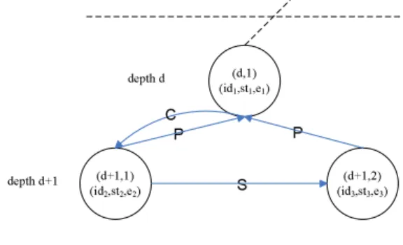
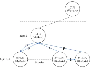
(16) 2. Find out all feasible starting times for each job instance. Once we choose a job to schedule it first, we might delay the starting time of it’s execution without missing it’s deadline. Each node of the tree is represented by a three-tuple: (id, st, e), where id is the identity (ID) of the job jobi , st is the valid start execution time for this job instance without missing it’s deadline, and e is the total energy consumption of the whole system until the complete time of the execution of this job instance (i.e., the total energy consumption of the interval from time 0 to the finish time of this job). Each node will be labelled by the coordinate (x, y) which means this node is the y-th node of depth x.. (d,1) (id 1,st1,e 1). depth d. P depth d+1. C. (d+1,1) (id 2,st2,e2). Figure 4.1: The parent node and the oldest child node. As shown in Figure 4.1, an edge P links two nodes node1 (id1 ,st1 ,e1 ) and node2 (id2 ,st2 ,e2 ) if the job with ID id2 can be successfully scheduled at time st2 after the job with ID id1 already scheduled at time st1 . The first child node of those nodes linked from the current parent node is the oldest child node and an edge C links to the first child node from the parent node.. (d,1) (id 1,st1,e 1). depth d. C P depth d+1. P. (d+1,1) (id2,st2,e 2). S. (d+1,2) (id 3,st3,e 3). Figure 4.2: Append the second child node. As shown in Figure 4.2, the second child node node3 (id3 ,st3 ,e3 ), which can successfully scheduled at time st3 after job id1 already scheduled at time st1 , is the younger sibling node of the first child node, an edge S links from older sibling node to the younger sibling node, and so on.. 13.

(17) (0,0) (id 1,st1,e 1). (d,1) depth d. C. depth d+1. (id 2,st2,e2). P. P. P. (d+1,1). (d+1,M+1). (id 3,st3,e 3). (id 4,st4,e 4). M nodes. S. (d+1,M+2) (id 5,st5,e 5). Figure 4.3: The coordinate of the search tree example. Figure 4.3 presents the coordinate of the search tree example. The first node on depth d was labelled with node(d, 1), the first node on depth (d + 1) was labelled with node(d + 1, 1), the M -th younger sibling node of node(d + 1, 1) was labelled with node(d + 1, M + 1), and so on. The procedure code of our BSTEE algorithm is shown in Algorithm 1. Algorithm 1 describes the main BSTEE algorithm scheme which can derive the completed schedule tree with the minimal energy consumption. Table 4.1 shows the definitions of notations which are used in Algorithm 1. At first, in lines 2 and 3, we generate a sorted job list which are partitioned by the (m, k)-firm pattern e.g., DR, ED or RED, and then initial a special node ROOT with coordinate (0,0). In lines 8-43, the main while loop is repeated until the depth of search tree is equal to the numbers of jobs, which means all jobs in the job list was scheduled. In lines 9, a temporarily un-scheduled job list was created which copy from the un-scheduled job list of the parent node. In lines 10-32, we try to find out all possible execution order from the job list and all feasible start execution time for each job instance, and then create a node to record relative information. In lines 44-45, finally we can identify the whole system schedule order and which job should be executed at what time. Next we will demonstrate the generation of the tree by using the job set shown in Table 3.5, and the device power consumption parameter was shown in Table 3.2. job1 and job2 are both released at time 0, job1 can be scheduled at t = 0, t = 1, or t = 2, and job2 can be also scheduled at t = 0, t = 1, or t = 2 without missing their deadlines. job3 and job4 were released at time 4 and 8. job3 can be scheduled at t = 4, t = 5, or t = 6 without missing it’s deadline while job4 can be scheduled at t = 6, t = 7, or t = 8 without missing it’s deadline. So, we can find 12 kinds of different execution orders from the ROOT node. After the energy consumptions were. 14.

(18) Algorithm 1 BASIC S EARCH T REE BASED E NERGY E FFICIENT A LGORITHM (task set T ) 1: Set y = 1, d = 1; 2: Use an (m,k)-firm partition policy to generate a job list for the task set T in the Hyper-Period; 3: Let the original un-scheduled job list lorg be the sorted job list by an ascending order of arrival time; 4: Initialize a special node as the tree root node ROOT , fill the attribute tuple as (0,0,0) and labelled with coordinate(0, 0); 5: Set the current parent node nodecp as the node ROOT ; 6: Let the un-scheduled job list l of the node ROOT be the original un-scheduled job list lorg ; 7: Set the link from the older sibling node to the younger sibling node S of the node ROOT as N U LL; 8: while d ≤ n do 9: Let the temporarily un-scheduled job list ltemp be the un-scheduled job list l of the current parent node nodecp; 10: for Each job ji ∈ the temporarily un-scheduled job list ltemp do 11: Find all feasible starting time set STi of job ji ; 12: if Can’t find any feasible starting time set STi of job ji then 13: Go to Lines 33; 14: end if 15: for Each time instance st ∈ set STi do 16: Create a node which labelled with coordinate(d, y); 17: Create the link from the child node to the parent node P from the node(d, y) to the current parent node nodecp; 18: if y == 1 then 19: Create the link from the parent to the oldest child node C from the current parent node nodecp to the node node(d, y); 20: Let the node node(d, y) be the current older sibling node nodecb; 21: Set the link from the older sibling node to the younger sibling node S of the node(d, y) as N U LL; 22: else 23: Create the link from the older sibling node to the younger sibling node S from the node nodecb to the node node(d, y); 24: Set the current older sibling node nodecb as the node node(d, y); 25: Set the link from the older sibling node to the younger sibling node S of the node(d, y) as NULL; 26: end if 27: Calculate the total energy consumptions e; 28: Fill up the tree-tuple (Ji , st, e) of the node(d, y); 29: Set the un-scheduled job list l of the node(d, y) as the temporarily un-scheduled job list ltemp exclude the job ji ; 30: y++; 31: end for 32: end for 33: if The link from the older sibling node to the younger sibling node S of the nodecp ̸= N U LL then 34: Set the current parent node nodecp as the link S of the current parent node nodecp; 35: else 36: if The link from the parent to the oldest child node C of the nodecp == NULL then 37: exit(0); (job list un-schedulable) 38: else 39: Set the current parent node nodecp as the link from the parent to the oldest child node C of the nodecp; 40: d++; 41: end if 42: end if 43: end while 44: Find the node noded, y in depth n with the minimal energy consumption emin ; 45: Record the path which is traced back to ROOT node from noded, y; and reverse the information of nodes in the path as the starting times of the corresponding job in the job list.. 15.

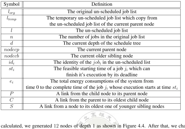
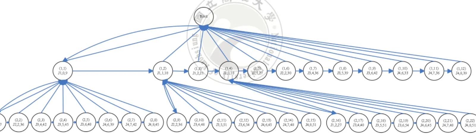
(19) Table 4.1: Definitions of Notations Symbol lorg ltemp l n d nodecp nodecb idi sti ei P C S. Definition The original un-scheduled job list The temporary un-scheduled job list which copy from the un-scheduled job list of the current parent node The un-scheduled job list The number of jobs in the original job list The current depth of the schedule tree The current parent node The current older sibling node The identity of the jobi in the un-scheduled list The feasible starting time of a job ji which can finish it’s execution by its deadline The total energy consumptions of the system from time 0 to the complete time of the job ji whose execution starts at time sti A link from the child node to its parent node A link from the parent to its oldest child node A link from a node to its oldest one of younger sibling nodes. calculated, we generated 12 nodes of depth 1 as shown in Figure 4.4. After that, we change the first child node of the current parent node ROOT : node(1, 1) as the current parent node because the node ROOT has no sibling nodes. Root. (1,1) J1,0,9. (1,2) J1,1,18. (1,3) J1,2,21. (1,4) J2,0,18. (1,5) J2,1,27. (1,6) J2,2,30. (1,7) J3,4,36. (1,8) J3,5,39. (1,9) J3,6,42. (1,10) J4,6,33. (1,11) J4,7,36. Figure 4.4: The BSTEE search tree of depth 1. Next we are going to process the depth 2 of the search tree. The first un-scheduled job in the un-scheduled job list l of node(1, 1) is job2 . job2 can be scheduled at t = 1 or t = 2 after job1 has been scheduled at t = 0 without missing it’s deadline. The second un-scheduled job in the un-scheduled job list l of node(1, 1) is job3 . job3 can scheduled at t = 4, t = 5, or t=6 after job1 has been scheduled at t = 0, and so on, 8 feasible child nodes of the node(1, 1) are generated.. 16. (1,12) J4,8,39.

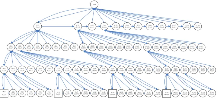
(20) Then we set the younger sibling node node(1, 2) of the node node(1, 1) as the current parent node nodecp . The first un-scheduled job in the un-scheduled job list l of node(1, 2) is job2 , and job2 can be scheduled at t = 2, and so on, 7 feasible child nodes of the node(1, 2) are created. The first un-scheduled job in the l of the node(1, 3) is also job2 , but we can’t find any feasible starting time for job2 because the deadline of job2 is 4. If any job in the unschedule job list will miss deadline, we can ignored this job execute order. We can’t generate any feasible child node for the other nodes except the node node(1, 4). Finally, we generated 22 nodes for depth 2 as shown in Figure 4.5. Figure 4.6 shows the search tree of depth 3. After the generation of the complete tree as shown in Figure 4.7, we can observe that node(4, 1), node(4, 7), node(4, 13) and node(4, 10) have the minimal energy consumptions 84. Then we can trace the tree link back from these node’s parent node to the ROOT node, and then reverse the path as a information to identify the whole system schedule order and which job should be executed at what time. For example, if we trace a path from the node(4, 19) to the ROOT node, we can get an execution schedule (j2 , 0) - (j1 , 2) - (j3 , 4) - (j4 , 6) with minimal energy consumptions 84. The execution schedule represents that j2 will be executed at time 0, j1 will be executed at time 2, j3 will be executed at time 4, and j4 will be executed at time 6. Root. (1,1) J1,0,9. (2,1) J2,1,27. (2,2) J2,2,36. (2,3) J3,4,42. (2,4) J3,5,45. (1,2) J1,1,18. (2,5) J3,6,48. (2,6) J4,6,39. (2,7) J4,7,42. (2,8) J4,8,45. (1,3) J1,2,21. (2,9) J2,2,36. (2,10) J3,4,48. (1,4) J2,0,18. (2,11) J3,5,51. (1,5) J2,1,27. (2,12) J3,6,54. (2,13) J4,6,45. (1,6) J2,2,30. (2,14) J4,7,48. (1,7) J3,4,36. (2,15) J4,8,51. (1,8) J3,5,39. (2,16) J1,2,27. (1,9) J3,6,42. (2,17) J3,4,48. (2,18) J3,5,51. (1,10) J4,6,33. (2,19) J3,6,54. (1,11) J4,7,36. (2,20) J4,6,45. Figure 4.5: The BSTEE search tree of depth 2.. 4.2 Advance Search-Tree-based Energy-Efficient Algorithm Next we will propose the advance search-tree-based energy-efficient algorithm (ASTEE) to reduce the tree size by adding two pruning constraints into the algorithm BSTEE : DeadlinePrune and Energy-Prune. The procedure code of our ASTEE algorithm is similar with the BSTEE algorithm as show in Algorithm 2. The pseudocode of pruning ideas are shown in Algorithm 3, and Algorithm 4. Algorithm 2 describes the main scheme of the ASTEE algorithm.. 17. (1,12) J4,8,39. (2,21) J4,7,48. (2,22) J4,8,51.

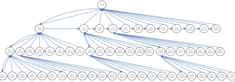
(21) Root. (1,1) J1,0,9. (2,1) J2,1,27. (3,1) J3,4,54. (3,2) J3,5,57. (2,2) J2,2,36. (2,3) J3,4,42. (3,3) J3,6,60. (3,4) J4,6,51. (2,4) J3,5,45. (3,5) J4,7,54. (1,2) J1,1,18. (2,5) J3,6,48. (3,6) J4,8,57. (2,6) J4,6,39. (3,7) J3,4,54. (2,7) J4,7,42. (3,8) J3,5,63. (2,8) J4,8,45. (3,9) J3,6,66. (1,3) J1,2,21. (2,9) J2,2,36. (3,10) J4,6,57. (2,10) J3,4,48. (3,11) J4,7,60. (1,4) J2,0,18. (2,11) J3,5,51. (1,5) J2,1,27. (2,12) J3,6,54. (3,12) J4,8,63. (3,13) J3,4,54. (1,6) J2,2,30. (2,13) J4,6,45. (3,14) J3,5,63. (2,14) J4,7,48. (3,15) J3,6,66. (1,7) J3,4,36. (2,15) J4,8,51. (3,16) J4,6,57. (1,8) J3,5,39. (2,16) J1,2,27. (3,17) J4,7,60. (1,9) J3,6,42. (2,17) (3,4,48. (3,18) J4,8,63. (1,10) J4,6,33. (2,18) J3,5,51. (3,19) J3,4,54. (2,19) J3,6,54. (3,20) J3,5,57. (1,11) J4,7,36. (2,20) J4,6,45. (3,21) J3,6,60. (1,12) J4,8,39. (2,21) J4,7,48. (2,22) J4,8,51. (3,22) J4,6,51. (3,23) J4,7,54. (3,24) J4,8,57. Figure 4.6: The BSTEE search tree of depth 3. At lines 40 and 41, after the node generation of a depth d in the schedule tree was completed, the deadline-prune procedure and the energy-prune procedure are performed to eliminate the non-necessary nodes. Algorithm 3 is the deadline-prune function. We check every job in the un-scheduled job list of each node of depth d. If any one of them will miss it’s deadline, then we can delete the node. Algorithm 4 describes the energy prune function. If there are two nodes have the same id and the same start time st in the depth d, and the domain of the previous scheduled jobs along these two node are the same too, then we can delete the node with higher energy consumption. We apply the ASTEE algorithm to the scheduling of the same job set as shown in Table 3.5. After the generation of the depth 1 in the search tree was finished, only three nodes, i.e., node(1, 1), node(1, 2), and node(1, 4), will not be pruned because any job in the un-scheduled job lists will miss it’s deadline, as shown in Figure 4.8. Next, 22 feasible nodes of the depth 2 in the search tree are generated. However, the deadline-prune function prunes 19 nodes, i.e., node(2, 3), node(2, 4), node(2, 5), node(2, 6), node(2, 7), node(2, 8), node(2, 10), node(2, 11), node(2, 12), node(2, 13), node(2, 14), node(2, 15), node(2, 17), node(2, 18), node(2, 19), node(2, 20), node(2, 21) and node(2, 22). node(2, 2) and node(2, 9) represent that j2 can start to be executed at t = 2 after j1 is scheduled. So we can delete node(2, 9) with a higher coordinate index, as shown in Figure 4.9. Figure 4.10 shows that, after the node generation of depth 3, node(3, 4), node(3, 5), node(3, 6), node(3, 10), node(3, 11), node(3, 12), node(3, 22), node(3, 23) and node(3, 24) will be pruned by the deadline-prune function. node(3, 7), node(3, 8), node(3, 9), node(3, 19), node(3, 20) and node(3, 21) will be pruned by the energy-prune algorithm. After the generation of the. 18.

(22) Algorithm 2 A DVANCE S EARCH T REE BASED E NERGY E FFICIENT A LGORITHM (task set T ) 1: Set y = 1, d = 1; 2: Use an (m,k)-firm partition policy to generate a job list for the task set T in the Hyper-Period; 3: Let the original un-scheduled job list lorg be the sorted job list by an ascending order of arrival time; 4: Initialize a special node as the tree root node ROOT , fill the attribute tuple as (0,0,0) and labelled with coordinate(0, 0); 5: Set the current parent node nodecp as the node ROOT ; 6: Let the un-scheduled job list l of the node ROOT be the original un-scheduled job list lorg ; 7: Set the link from the older sibling node to the younger sibling node S of the node ROOT as N U LL; 8: while d ≤ n do 9: Let the temporarily un-scheduled job list ltemp be the un-scheduled job list l of the current parent node nodecp; 10: for Each job ji ∈ the temporarily un-scheduled job list ltemp do 11: Find all feasible starting time set STi of job ji ; 12: if Can’t find any feasible starting time set STi of job ji then 13: Go to Lines 33; 14: end if 15: for Each time instance st ∈ set STi do 16: Create a node which labelled with coordinate(d, y); 17: Create the link from the child node to the parent node P from the node(d, y) to the current parent node nodecp; 18: if y == 1 then 19: Create the link from the parent to the oldest child node C from the current parent node nodecp to the node node(d, y); 20: Let the node node(d, y) be the current older sibling node nodecb; 21: Set the link from the older sibling node to the younger sibling node S of the node(d, y) as N U LL; 22: else 23: Create the link from the older sibling node to the younger sibling node S from the node nodecb to the node node(d, y); 24: Set the current older sibling node nodecb as the node node(d, y); 25: Set the link from the older sibling node to the younger sibling node S of the node(d, y) as NULL; 26: end if 27: Calculate the total energy consumptions e; 28: Fill up the tree-tuple (Ji , st, e) of the node(d, y); 29: Set the un-scheduled job list l of the node(d, y) as the temporarily un-scheduled job list ltemp exclude the job ji ; 30: y++; 31: end for 32: end for 33: if The link from the older sibling node to the younger sibling node S of the nodecp ̸= N U LL then 34: Set the current parent node nodecp as the link S of the current parent node nodecp; 35: else 36: if The link from the parent to the oldest child node C of the nodecp == NULL then 37: exit(0); (job list un-schedulable) 38: else 39: Set the current parent node nodecp as the link from the parent to the oldest child node C of the nodecp; 40: Deadline-Prune(d); 41: Energy-Prune(d); 42: d++; 43: end if 44: end if 45: end while 46: Find the node noded, y in depth n with the minimal energy consumption emin ; 47: Record the path which is traced back to ROOT node from noded, y; and reverse the path as the starting times of the corresponding job in the job list;. Algorithm 3 D EADLINE -P RUNE (depth d) 1: 2: 3: 4: 5: 6: 7:. for Every node n1 in depth d do for Each un-scheduled job ji in the un-scheduled job list l of the node n1 do if Any one of the un-scheduled job ji will miss deadline then Delete the node n1 ; end if end for end for. 19.

(23) Root. (1,1) J1,0,9. (2,1) J2,1,27. (2,2) J2,2,36. (2,3) J3,4,42. (2,4) J3,5,45. (1,2) J1,1,18. (2,5) J3,6,48. (2,6) J4,6,39. (2,7) J4,7,42. (2,8) J4,8,45. (1,3) J1,2,21. (2,9) J2,2,36. (2,10) J3,4,48. (1,4) J2,0,18. (2,11) J3,5,51. (1,5) J2,1,27. (2,12) J3,6,54. (1,6) J2,2,30. (2,13) J4,6,45. (2,14) J4,7,48. (1,7) J3,4,36. (2,15) J4,8,51. (1,8) J3,5,39. (2,16) J1,2,27. (1,9) J3,6,42. (2,17) (3,4,48. (1,10) J4,6,33. (2,18) J3,5,51. (2,19) J3,6,54. (1,11) J4,7,36. (2,20) J4,6,45. (1,12) J4,8,39. (2,21) J4,7,48. (2,22) J4,8,51. (3,1) J3,4,54. (3,2) J3,5,57. (3,3) J3,6,60. (3,4) J4,6,51. (3,5) J4,7,54. (3,6) J4,8,57. (3,7) J3,4,54. (3,8) J3,5,63. (3,9) J3,6,66. (3,10) J4,6,57. (3,11) J4,7,60. (3,12) J4,8,63. (3,13) J3,4,54. (3,14) J3,5,63. (3,15) J3,6,66. (3,16) J4,6,57. (3,17) J4,7,60. (3,18) J4,8,63. (3,19) J3,4,54. (3,20) J3,5,57. (3,21) J3,6,60. (3,22) J4,6,51. (3,23) J4,7,54. (3,24) J4,8,57. (4,1). (4,2) J4,7,72. (4,3) J4,8,75. (4,4) J4,7,66. (4,5) J4,8,75. (4,6) J4,8,69. (4,7) J4,6,63. (4,8) J4,7,72. (4,9) J4,8,74. (4,10) J4,7,72. (4,11) J4,8,81. (4,12) J4,8,75. (4,13) J4,6,63. (4,14) J4,7,72. (4,15) J4,8,75. (4,16) J4,7,72. (4,17) J4,8,81. (4,18) J4,8,75. (4,19) J4,6,63. (4,20) J4,7,72. (4,21) J4,8,75. (4,22) J4,7,63. (4,23) J4,8,75. (4,24) J4,8,69. J4,6,63. Figure 4.7: The BSTEE completed schedule tree. Algorithm 4 E NERGY-P RUNE (depth d) 1: for Any two nodes n1 and n2 in depth d do 2: if n1 ’s id == n2 ’s id and n1 ’s st == n2 ’s st then 3: if The domain of the previously scheduled jobs along the n1 and n2 are the same then 4: if n1 ’s e == n2 ’s e then 5: Delete the node with higher coordinate index (x, y); 6: else 7: Delete the node with higher e; 8: end if 9: end if 10: end if 11: end for. search tree is completed, we can find that node(4, 1) has the minimal energy consumption 63, then we can trace the path back from node(4, 1) to the ROOT node to identify the schedule order in which each job should be executed at what time, as shown in Figure 4.11.We can observe that the ASTEE algorithm is more efficient than the BSTEE algorithm and uses less space during the generation of the schedule tree.. 20.

(24) / Prune with deadline constraint \ Prune with energy constraint. Root. (1,1) J1,0,9. (1,2) J1,1,18. (1,4) J2,0,18. (1,3) J1,2,21. (1,5) J2,1,27. (1,6) J2,2,30. (1,7) J3,4,36. (1,8) J3,5,39. (1,9) J3,6,42. (1,10) J4,6,33. (1,11) J4,7,36. (1,12) J4,8,39. Figure 4.8: The ASTEE search tree of depth 1.. Root. (1,1) J1,0,9. (2,1) J2,1,27. (2,2) J2,2,36. (2,3) J3,4,42. (2,4) J3,5,45. / Prune with deadline constraint \ Prune with energy constraint. (1,2) J1,1,18. (2,5) J3,6,48. (2,6) J4,6,39. (2,7) J4,7,42. (2,8) J4,8,45. (2,9) J2,2,36. (2,10) J3,4,48. (1,4) J2,0,18. (2,11) J3,5,51. (2,12) J3,6,54. (2,13) J4,6,45. (2,14) J4,7,48. (2,15) J4,8,51. (2,16) J1,2,27. (2,17) J3,4,48. (2,18) J3,5,51. (2,19) J3,6,54. Figure 4.9: The ASTEE search tree of depth 2.. Root. / Prune with deadline constraint \ Prune with energy constraint. (3,1) J3,4,54. (3,2) J3,5,57. (3,3) J3,6,60. (3,4) J4,6,51. (3,5) J4,7,54. (3,6) J4,8,57. (3,7) J3,4,54. (1,1) J1,0,9. (1,2) J1,1,18. (1,4) J2,0,18. (2,1) J2,1,27. (2,2) J2,2,36. (2,16) J1,2,27. (3,8) J3,5,63. (3,9) J3,6,66. (3,10) J4,6,57. (3,11) J4,7,60. (3,12) J4,8,63. (3,19) J3,4,54. (3,20) J3,5,57. Figure 4.10: The ASTEE search tree of depth 3.. 21. (3,21) J3,6,60. (3,22) J4,6,51. (3,23) J4,7,54. (3,24) J4,8,57. (2,20) J4,6,45. (2,21) J4,7,48. (2,22) J4,8,51.

(25) Root. (4,1) J4,6,63. / Prune with deadline constraint \ Prune with energy constraint. (1,1) J1,0,9. (1,2) J1,1,18. (1,4) J2,0,18. (2,1) J2,1,27. (2,2) J2,2,36. (2,16) J1,2,27. (3,1) J3,4,54. (3,2) J3,5,57. (3,3) J3,6,60. (4,2) J4,7,72. (4,3) J4,8,75. (4,4) J4,7,66. (4,5) J4,8,75. (4,6) J4,8,69. Figure 4.11: The ASTEE completed schedule tree.. 22.

(26) Chapter 5 Performance Evaluation The purpose of this chapter is to evaluate the performance of the proposed BSTEE algorithm and the ASTEE algorithm. We develop a simulation model for the proposed BSTEE algorithm and the ASTEE algorithm, and use some numerical examples to show the capabilities of the proposed algorithms.. 5.1 Experiment Setup and Performance Metrics In our experiments, we compare the performance of the ASTEE algorithm and the BSTEE algorithm which does not adopt any conditions to prune the node generation. We design a task generator to produce periodic tasks and their workload for each experimental task set. The performance of our ASTEE algorithm is inspected on a large number of task sets by the energy consumption. Each set of parameters randomly generated 100 task sets. Therefore, each simulation result is an average value over these 100 independent task sets. In order to guarantee the (m, k) constraints, we adopt the DR, ED, and RED schemes. The numbers of tasks in a tested task set are 1, 2, 3, and 4. The deadline of each task is equal to it’s period. The period of each task is randomly selected from {2, 3, 4, 5, 6, 8, 9, 10, 12}. The worst-case execution time of each task in a task set is generated by a random variable with the range of 1 and the corresponding deadline. The original total task utilization of each experimental task set is 1.0, and we choose three different kinds of (m, k) settings, i.e., (3,10), (6,10), and (9,10). Table 5.1 shows our power consumption parameters of experiment which was based on [14]. The primary performance metrics are the normalized energy consumption, the number of generated nodes, and the number of physical required nodes. The normalized energy consumption is defined as the ratio of the energy consumption derived by the proposed ASTEE algorithm divided by the same execution order without device shutdown policy. The number. 23.

(27) Table 5.1: Power consumption parameters of experiment Device A Processor. Pa 0.3 0.63. Ps 0.1 0.25. Psd =Pwu 0.2 0.4. Tsd =Twu 1 1. of generated nodes is defined as the number of the nodes generated by the BSTEE algorithm. The number of physical required nodes is defined as the number of the generated nodes under the ASTEE algorithm.. 5.2 Experimental Results Figure 5.1 shows the normalized energy consumptions under of three different schemes, i.e., DR, ED, and RED when (m, k) = (3, 10). Note that the BSTEE algorithm and the ASTEE algorithm have the same experimental results. The difference between then is the size of the used memory space during the generation procedure of the schedule tree. This figure intuitively shows that the normalized energy consumption values for the DR and ED schemes, increase as the number of the tasks int a tested task set increases. However, the RED scheme has the similar results under different task numbers. The reason is that the number of mandatory jobs for a task set increases as the task number of the task set. Each job has it’s own arrival time and deadline, so the I/O device can not be used continuously by jobs, resulting in lower energy efficiency. The DR scheme has the better performance compared with the other schemes. The reason is that under the DR scheme, the first job of every task is always marked to be mandatory. So the mandatory jobs marked by the DR scheme are always more concentrated than the other schemes. The mandatory jobs marked by the RED scheme are more evenly distributed and the arrival time are later than those of the mandatory jobs marked by the ED and DR schemes. In other words, the system requires longer time to complete all of mandatory jobs, resulting in higher total energy consumption become larger. Figures 5.2 and 5.3 shows the normalized energy consumptions under of three different schemes, i.e., DR, ED, and RED when (m, k) = (6, 10) and (9, 10), respectively. Comparing Figures 5.1, 5.2, and 5.3, we can observe that when (m, k) = (9, 10), the normalized energy consumption is higher. The reason is that the task set under (m, k) = (9, 10) has more mandatory jobs needed to be executed. The system load is higher. Such a higher system load leads to fewer idle intervals for shutdowning the I/O device and most time of a system is used to. 24.

(28) execute jobs. Besides, the DR scheme and the ED scheme have very similar performance. This is because the mandatory jobs marked by the DR scheme and the ED scheme are exactly the same. 1. no it p m us no C yg re nE de zli a m ro N. 0.9 0.8 0.7 0.6 0.5 0.4 0.3. Deeply Red Evenly Distributed Reversed Evenly Distributed. 0.2 0.1 0 1. 2. 3. 4. Task numbers Figure 5.1: The normalized energy consumption when (m,k) = (3,10) Figure 5.4 shows the number of generated nodes of the DR, ED, and RED schemes when (m, k) = (3, 10). We can observe that that the number of generated nodes for the DR, ED and RED schemes, increase as the number of the tasks int a tested task set increases. The reason is that if a task set has more tasks, there are more combinations of execution order for the job list of the task set. Besides, the three schemes have similar performance. However, the numbers of generated nodes of the RED scheme and the ED scheme are a bit bigger than those of the DR scheme. The reason is that the mandatory jobs of the RED scheme and the ED scheme are more evenly distributed. Such the property makes that a job can have more feasible time instances to start execution. Note that the RED scheme has the better performance than the ED scheme. The reason is that the mandatory jobs of the RED scheme is more evenly distributed than the ED scheme. Figures 5.5 and 5.6 show the numbers of generated nodes under the three different schemes, i.e., DR, ED, and RED when (m, k) = (6, 10) and (9, 10), respectively. We can observe that the number of generated nodes when (m, k) = (6, 10) is larger than that when (m, k) = (9, 10). The reason of this phenomenon is that when the system load is higher, it is harder to find feasible time instances for a job. Figure 5.7 shows the number of physically required nodes of the DR, ED, and RED schemes when (m, k) = (3, 10). The trend of the numbers of physically required nodes under. 25.

(29) no it p m us no C yg re nE de zil a m ro N. 1 0.9 0.8 0.7 0.6 0.5 0.4. Deeply Red Evenly Distributed Reversed Evenly Distributed. 0.3 0.2 0.1 0 1. 2. 3. 4. Task numbers Figure 5.2: The normalized energy consumption when (m,k) = (6,10) each scheme is similar to that of generated nodes under the same scheme. Compared with Figure 5.7, we can conclude that the ASTEE algorithm successfully save a lot memory space during the generation of the search. Figures 5.8 and 5.9 show the numbers of physically required nodes under of three different schemes, i.e., DR, ED, and RED when (m, k) = (6, 10) and (9, 10), respectively. We also can observe that the ASTEE algorithm uses less memory space.. 26.

(30) 1 0.9. no 0.8 it p m us 0.7 no C 0.6 yg ern 0.5 E de 0.4 izl a 0.3 rm oN. Deeply Red Evenly Distributed Reversed Evenly Distributed. 0.2 0.1 0 1. 2. 3. 4. Task Numbers. Figure 5.3: The normalized energy consumption when (m,k) = (9,10). 60000. se do N de ta re ne G fo re b m u N. Deeply Red Evenly Distributed Reversed Evenly Distributed. 50000 40000 30000 20000 10000 0 1. 2. 3. 4. Task numbers Figure 5.4: The number of generated nodes when (m,k) = (3,10). 27.

(31) 60000. se do N de ta re ne G fo re b m u N. Deeply Red Evenly Distributed Reversed Evenly Distributed. 50000 40000 30000 20000 10000 0 1. 2. 3. 4. Task numbers Figure 5.5: The number of generated nodes when (m,k) = (6,10). se do N de ta re ne G fo re b m u N. 60000. Deeply Red Evenly Distributed Reversed Evenly Distributed. 50000 40000 30000 20000 10000 0 1. 2. 3. 4. Task numbers Figure 5.6: The number of generated nodes when (m,k) = (9,10). 28.

(32) se do N de ri uq eR la cis yh Pf or eb m u N. 500. Deeply Red Evenly Distributed Reversed Evenly Distributed. 450 400 350 300 250 200 150 100 50 0 1. 2. 3. 4. Task numbers Figure 5.7: The number of physicaly required nodes when (m,k) = (3,10). se do N de ri uq eR la cis yh Pf or eb m u N. 500. Deeply Red Evenly Distributed Reversed Evenly Distributed. 450 400 350 300 250 200 150 100 50 0 1. 2. 3. 4. Task numbers Figure 5.8: The number of physically required nodes when (m,k) = (6,10). 29.

(33) se do N de ri uq eR la cis yh Pf or eb m u N. 500. Deeply Red Evenly Distributed Reversed Evenly Distributed. 450 400 350 300 250 200 150 100 50 0 1. 2. 3. 4. Task numbers Figure 5.9: The number of physically required nodes when (m,k) = (9,10). 30.

(34) Chapter 6 Conclusion In order to solve the scheduling problem of a weakly-hard real-time system with an I/O device, the basic search-tree-based energy-efficient (BSTEE) algorithm and the advanced search-treebased energy-efficient (ASTEE) algorithm are proposed. In the ASTEE algorithm, we adopt two prune ideas to reduce the schedule tree size. The ASTEE algorithm uses less memory space during the generation of the schedule tree compared with the BSTEE algorithm. An analytic study was developed for the proposed algorithm and was verified against the experimental results. A series of simulation experiments were conducted to show the capability of the proposed algorithm, for which we have very encouraging results. For the future work, we will tune up our methodology for the systems with multiple I/O devices. We will also start designing a new mechanism considering the I/O device with multiple different-level sleep states.. 31.

(35) Bibliography [1] Mazhar Alidina, Jos´e Monteiro, Srubuvas Devadas, Abhijit Ghosh, and Marios Papaefthymiou. Precomputation-based sequential logic optimization for low power. In IEEE Transactions on Very Large Scale Integration (VLSI) Systems, December 1994. [2] Hakan Aydin, Rami Melhem, Hakan Aydin, Daniel Mosse, and Pedro Mejia-Alvarez. Determining optimal processor speeds for periodic real-time tasks with different power characteristics. In Euromicro Conference on Real-time Ssystems, 2001. [3] Moncef Hamdaoui and Parameswaran Ramanathan. A dynamic priority assignment technique for streams with (m,k)-firm deadlines. IEEE Transactions on Computers, 44:1443– 1451, 1994. [4] Chi-Hong Hwang and Allen C.-H. Wu. A predictive system shutdown method for energy saving of event-driven computation. pages 28–32, 1997. [5] Ravindra Jejurikar and Rajesh K. Gupta. Dynamic slack reclamation with procrastination scheduling in real-time embedded systems. In William H. Joyner Jr., Grant Martin, and Andrew B. Kahng, editors, DAC, pages 111–116. ACM, 2005. [6] M. Tim Jones. Anatomy of linux process management. http://www.ibm.com/ developerworks/linux/library/l-linux-process-management/. [7] Woonseok Kim, Jihong Kim, and Sang Lyul Min. A dynamic voltage scaling algorithm for dynamic-priority hard real-time systems using slack time analysis. In Design Automation and Test in Europe, 2002. [8] G. Koren and D. Shasha. Skip-over: Algorithms and complexity for overloaded systems that allow skips. New York, NY, USA, 1996. New York University. [9] Jane W. S. Liu. Real-Time Systems. Prentice Hall, 2000.. 32.

(36) [10] Linwei Niu and Gang Quan. Energy minimization for real-time systems with (m; k)guarantee. IEEE Trans. Very Large Scale Integr. Syst., 14(7):717–729, July 2006. [11] Gang Quan and Xiaobo (Sharon) Hu. Enhanced fixed-priority scheduling with (m,k)-firm guarantee. In IEEE Real-Time Systems Symposium, pages 79–88, 2000. [12] P. Ramanathan. Overload management in real-time control applications using (m,k)-firm guarantee. IEEE Trans. On Paral. and Dist. Sys., 10(6):549–559, Jun. 1999. [13] Vishnu Swaminathan and Krishnendu Chakrabarty. Energy-conscious, deterministic i/o device scheduling in hard real-time systems. IEEE Transactions on Computer-aided Design of Integrated Circuits and Systems, 22(7):858, 2003. [14] Vishnu Swaminathan and Krishnendu Chakrabarty. Pruning-based, energy-optimal, deterministic i/o device scheduling for hard real-time systems. ACM Transactions on Embedded Computing Systems, 4(1):141–167, 2005. [15] Frances Yao, Alan Demers, and Scott Shenker. A scheduling model for reduced cpu energy. In IEEE Syposium on Foundations of Computer Science, 1995.. 33.

(37)