南部科學園區地盤震動量測與衰減特性之研究

行政院國家科學委員會專題研究計畫 成果報告

南部科學園區地盤震動量測與衰減特性之研究

研究成果報告(精簡版)

計 畫 類 別 ： 個別型

計 畫 編 號 ： NSC 95-2221-E-002-106-

執 行 期 間 ： 95 年 08 月 01 日至 96 年 07 月 31 日

執 行 單 位 ： 國立臺灣大學土木工程學系暨研究所

計 畫 主 持 人 ： 陳正興

計畫參與人員： 博士班研究生-兼任助理：黃宗辰、張為光

碩士班研究生-兼任助理：曹碩修、陳于純

報 告 附 件 ： 出席國際會議研究心得報告及發表論文

處 理 方 式 ： 本計畫可公開查詢

中 華 民 國 96 年 10 月 30 日

行政院國家科學委員會專題研究計畫成果報告

南部科學園區地盤振動量測與衰減特性之研究

Ground Vibration and Attenuation Characteristics

at Southern Taiwan Science Park

計畫編號：NSC 95-2211-E-002-106

執行期限：95 年 8 月 1 日至 96 年 7 月 31 日

主持人：陳正興 國立臺灣大學土木工程學研究所

壹、中文摘要

穿越南部科學園區之台灣高速鐵路已

全面通車，其所引致之地盤振動，對周圍

高科技廠房具有一定之影響，而園區內地

盤振動特性與之有密切的關係。

本研究係針對南部科學園區內高鐵行

經區域，進行一系列現地振動量測與分

析，分析內容除了針對先前已於南科園區

內進行之重錘落擊振動試驗與起振器強迫

振動試驗進行分析外，再加入實際高鐵列

車以及園區內各類重車通過引致振動之量

測分析。藉由對不同振源形式所引致振動

之地盤進行分析，可更加有系統的對園區

內振動特性有所掌握，並確切比較出各類

振動形式對地盤動態反應以及振動衰減情

形之差異。

關鍵詞：高速鐵路、南科園區、地盤振動

特性、振動衰減係數

Abstract

The Taiwan High Speed Rail (THSR) passes through the Southern Taiwan Science Park (STSP). The ground vibration induced by trains

of THSR influence high-tech factories and

equipments inside the STSP and it will effects the ground vibration properties. Therefore, it is very important to deeply grasp the ground vibration properties.

In this study, we made a series of in-site

measurement and analyses of vibration. Analyzed content includes previous tests of drop hammer and shaker vibration, and also contains subsequent tests of the vibration induced by trains. We can catch the ground vibration properties more systematically by analyzing different vibrating sources, and difference dynamic responses and the attenuation of ground vibration from various sources.

Keywords:

High Speed Rail, STSP, Ground Vibration, Attenuation Coefficient.

貳、前言

「台南科學園區」之設置與「高速鐵

路」之興建均為政府重大公共建設計畫，

對於整體經濟景氣帶動與發展，具有相當

的正面效益；然而沿台灣西部走廊興建中

之台灣高速鐵路工程，其行車路線穿越設

置於台南縣新市附近之南部科學園區，園

區已設置有微電子精密機械、半導體與農

產生物技術等專業區，專業區內之高科技

產業對地盤振動之影響甚為敏感，高鐵列

車行經此地勢必引起一定之地盤振動，因

此對科學園區廠房造成之振動影響也成為

各界關心之焦點。

本計劃之目的在於探討南科園區地盤

之振動特性以及地盤之振動衰減特性，因

此在本研究中，除了於高鐵試車期間於南

科園區內進行不同車速之高鐵列車通過引

致地表振動之量測與分析，並整合以往在

南科園區內進行之一系列相關振動試驗資

料(包含重錘落擊落試驗、起振器強迫振動

試驗…等，相關試驗位置與內容如圖 1 與

表

1 所示)，將各種試驗所得地盤動態特性

及衰減特性進行差異探討。

另外影響南科園區內，致使地表振動

產生的另一個主要振動源，即為往來南北

的重車，其通過時所造成之振動量，不亞

於高鐵列車之影響，因此在本研究中特別

將之納入振動量測分析之範圍，除了可進

一步瞭解重車通過時所引致振動之特性

外，亦可更進一步探討其所引致振動對高

科技廠房可能產生之影響。

經由以上所提之各種分析，則可更精

確掌握南科園區內地盤受到不同形式振源

作用下，其動態反應以及波傳衰減之特

性，並可做為未來園區內高科技廠房進行

隔減振結構設計之參考。

參、振動之頻譜分析

量測所紀錄資料之處理方式與分析流

程如圖

2 所示，概述如下：

速度頻譜之計算以三分之一倍頻寬

(1/3 Octave) 速 度 平 方 之 平 均 方 根 值

RMS(Root Mean Square)為準，實際採用之

中 心 頻 率 與 其 上 下 限 係 根 據

ANSI S1.

6-1984 所訂之標準值。1/3 倍頻頻帶頻譜

(One-Third-Octave-Banded RMS Amplitude

Spectra)係以分貝(dB)表示 RMS 速度振動

量。茲將其計算步驟簡述如后。

若量測所得之速度反應歷時為

v(t)，先

將 其 經 由 傅 利 葉 轉 換 求 得 傅 氏 譜 振 幅

V(f)，則其單邊功率頻譜密度函數(Power

Spectrum Density Function)S(f)可由下式求

得：

T

f

V

f

S

2

)

(

2

)

(

=

(1)

其中

T 為速度歷時之等效穩態延時

T

eff

，需注意的是

T

eff

應包含實際有效振動之

延時，並不包含快速傅利葉轉換時所補之

零。對應中心頻率為

fi 之 1/3 倍頻頻帶內之

振動含量為：

=

∫

u i l i f f i

S

f

df

f

E

(

)

(

)

(2)

上式中

f

il

與

f

iu

為為對應於中心頻率為

f

i

之上下限頻率。在每一頻寬內，速度振動

量之均方根值(RMS)σ(f

i

)為

σ

(

f

_i

)

=

E

(

f

_i

)

(3)

再由下式可計算相對於參考速度

v

0

之

振動分貝(dB)值為 L(fi)：

0 10

)

(

log

20

)

(

v

f

f

L

i i

σ

⋅

=

(4)

上式中

v

0

為參考速度，本計劃所用之

v

0

=10

-6

in/sec，為晶圓廠振動規範常用之標

準參考值。

肆、振動衰減係數

本研究中依不同的振源形式進行振動

衰減係數分析，重錘落擊試驗、起振器

(Shaker)強迫振動試驗與重車引致之地盤振

動屬於點振源形式，而列車通過時所引致之

振動則屬於線振源的形式，其衰減係數之分

析方法分別說明如下：

A. 點振源之振動衰減係數

重錘落擊試驗、起振器(Shaker)強迫振

動試驗與重車引致地盤振動之情形，相當於

在地表面上施加一點振源，在不同距離處量

測所得之地表振動可視為點振源所造成之

Rayleigh wave，其振幅衰減關係可用下式表

示：

(5)

上式中，

V

1

為距振源

r

1

處之振幅，

V

2

為距

振源

r

2

處之振幅，α為地層材料之振動衰

減係數。

B. 線振源之振動衰減係數

列車在經過測線時所引致地盤振動情

形，相當於在地表面上施加一時間歷時之線

振源，在不同距離處量測所得之地表振動可

視為線振源所造成之

Rayleigh wave，其振幅

衰減關係可用下式表示：

) ( 1 2 2 1 r r

e

V

V

=

⋅

−α −

₍₆₎

上式中符號之定義與點振源振動衰減係數

公式之符號定義相同。

伍、振動量測分析結果

A. 重錘落擊試驗

1. 振幅情形

經過振動資料之處理，可得到各測點

振幅之1/3倍頻帶均方根速度值(dB)。如圖3

中所示，為試驗B(43t重錘，3m落距)在距

振源不同距離之水平徑向與垂直方向上反

應，由圖中顯示各頻率之振幅皆有明顯隨

距離衰減之情形。

2. 振動衰減係數

圖

4 為重錘落擊試驗所得衰減係數之

情形，結果整理如下：

(1) 當錘重愈重，落擊時產生之能量愈大，

其 所 得 到 之 振 動 衰 減 係 數 會 相 對 較

小，即表示所產生之地盤振動會愈不易

衰減。

(2) 在淺基礎上進行重錘落擊試驗所得之

地盤振動衰減係數與在素地上進行試

驗所得者非常接近；於單樁基礎上進行

重錘落擊試驗所得之地盤振動衰減係

數則相對較前述兩者小。

(3) 在較低頻率時 ( f < 10Hz)，振動之衰減

較慢(α≒0.002~0.01(1/m))；而在較高頻

率時(f > 10Hz)，振動之衰減則相對較快

速(α≒0.0035~0.02(1/m))。

B. 起振器振動試驗

1. 振幅情形

經過振動資料之處理，可得到各測點

之均方根速度振幅值(dB)。圖5與圖6所示

分別為在試驗F中進行水平橫向出力試驗

(HT試驗)與水平徑向出力試驗(HL試驗)

時，在距振源不同距離之水平方向與垂直

方向反應，由圖中顯示各頻率之振幅皆有

隨距離衰減之情形，其中又以水平方向之

情形較為明顯。

2. 振動衰減係數

a. 水平橫向出力試驗(HT-test)(如圖7所

示

)

(1) 在 HT-test 中各測點所量得之地盤振動

屬於

Love wave 之型式，因此主要係針

對水平橫向振動來進行分析。

(2) 就各種型式之基礎而言，在振動頻率小

於

6Hz 時，衰減係數主要介於 0.0006~

0.003(1/m)之間；而當振動頻率高於 6Hz

時，衰減係數會有隨振動頻率提高而增

加之情形。

b. 水平徑向出力試驗(HL試驗) (如圖8所

示)

(1) 在 HL-test 中各測點所量得之地盤振動

屬於

Rayleigh wave 之型式，因此主要

係針對水平徑向與鉛錘向振動來進行

分析。

(2) 在淺基礎上試驗或起振器出力方向平

行於群樁基礎樁帽的短向上時，水平方

) ( 2 1 1 2 2 1 r r e r r V V = ⋅ −α −

向之地盤振動衰減係數會有隨振動頻

率提高而略有增加之情形；但在單樁基

礎上試驗或起振器出力方向平行於群

樁基礎樁帽的長向上時，水平方向之振

動衰減係數則會有隨振動頻率提高而

有降低之情形。

(3) 不論是在何種型式之基礎上進行 HL 試

驗，鉛錘方向之地盤振動衰減係數皆會

有隨振動頻率提高而有增加之趨勢。

(4) 在淺基礎上進行起振器強迫振動試驗

所得到之衰減係數，不論在水平向上或

鉛錘向上，皆明顯較在樁基礎(包含單

樁與群樁基礎)上試驗所得到者要高。

(5) 在振動頻率低於 10Hz 時，水平向之衰

減係數皆較鉛錘向之衰減係數高。

C. 高鐵列車通過時引致振動量測

1. 振幅情形

採用與重錘落擊試驗相同之分析步

驟，可推求出高鐵列車通過時引致地盤振

動之1/3倍頻帶均方根速度值(dB)。圖9所示

為距離高鐵鐵道不同位置之測點下，三方

向(包括 X、Y與Z方向)之振動反應情形。

根據結果顯示，當振動頻率在2.5Hz以上

時，在各振動頻率下皆有較為明顯振幅隨

距離衰減之情形。

2. 振動衰減係數

衰減係數

α 可由式(6)推求出。圖 10~12

左側圖為各方向上不同車速下

α 值之情

形。分析結果簡述如下：

(1) 由高鐵列車通過引致地盤振動所求得

之衰減係數，有明顯隨頻率增加而提高

之情形。

(2) 在X、Y與Z三方向所得到之衰減係數皆

非常接近。

(3) 列車車速在240、270、290及300 km/hr

時，分析所得之衰減係數非常接近，可

以此趨勢線(如圖10~12右圖黑線表示)

來代表高鐵列車通過引致地盤振動之

衰減情形。

D. 重車通過引致振動量測

1. 振幅情形

同樣採用與重錘落擊試驗相同之分析

步驟，可推求出重車通過測線時，引致地

盤振動之1/3倍頻帶均方根速度值(dB)。如

圖13~圖15左側圖所示，為距重車振源不同

位置之測點，在三方向(X、Y與Z方向)各振

動頻率之振幅反應情形。

由分析結果顯示，重車之顯著振動頻

率主要集中在12.5Hz附近，而在低於10Hz

之振幅則相對較小，因此也較難以識別出

其振動衰減特性；而在振動頻率大於10Hz

時，在各方向則皆可明顯識別出振幅隨距

離衰減之情形。

2. 振動衰減係數

衰減係數 α 可由式(5)推求出。圖 13~

圖

15 中之右側圖為行駛於南科園區內重車

通過時所引致地盤振動，在各方向上

α 值

之情形。由分析之結果顯示，園區內重車

通過引致地盤振動之衰減係數，在振動頻

率

10Hz 以上時，各方向上皆略可識別屋其

隨頻率增加而提高之趨勢，尤其在

Y 方向

與

Z 方向上較為明顯。

陸、列車通過時引致地盤振動與其他振源

分析所得振動與衰減特性之比較

A. 重錘落擊試驗與高鐵列車通過時引致振

動分析結果之比較

圖

16 與圖 17 分別將重錘落擊試驗與

高鐵列車通過時引致地盤振動之振幅以及

衰減係數之比較結果整理如下：

(1) 如圖16所示，在大部份頻率下，高鐵列

車通過引致地盤振動幅度皆低於重錘

落擊試驗引致之地盤振動。

(2) 如圖17所示，高鐵列車通過引致地盤振

動在X向與Z向之衰減係數，皆有明顯低

於重鎚落擊試驗衰減係數之情形。

(3) 雖然兩者所得到之α值仍有差異，但兩

者衰減係數之回歸線則具有非常相近

之趨勢(如圖17所示)。

B. 起振器(shaker)試驗與高鐵列車通過時

引致振動分析結果之比較

圖

18~圖 20 分別將起振器強迫振動試

驗與高鐵列車通過時引致地盤振動之振幅

以及衰減係數之比較結果整理如下：

(1) 由圖18~圖20左側圖顯示，高鐵列車通

過時引致之地表振幅，在各方向上皆有

明顯小於起振器強迫振動試驗所產生

地表振幅之情形。

(2) 由圖18與圖20右側圖顯示，在大部份的

振動頻率下，高鐵列車通過時引致振動

之衰減係數，在X方向與Z方向上，皆有

明顯小於起振器強迫振動試驗所得振

動衰減係數之情形。

(3) 由圖19右側圖顯示在Y方向上，當振動

頻率低於10Hz時，高鐵列車通過時引致

振動之衰減係數，皆明顯高於起振器強

迫振動試驗所得振動衰減係數；而在振

動頻率高於10Hz時，則是低於起振器強

迫振動試驗所得振動衰減係數下之情

形，由此可見兩者引致地盤振動衰減特

性之差異。

(4) 由兩者之比較結果顯示，高鐵列車通過

引致地盤振動與衰減特性與起振器強

迫振動試驗所得到之結果，具有相當程

度的差異，因此起振器試驗之結果顯然

也較不適合用來模擬高鐵列車通過引

致地盤振動與衰減特性。

C. 重車通過與高鐵列車通過時引致振動分

析結果之比較

圖21與圖22所示分別為重車通過與高

鐵列車通過時引致地盤振動之振幅以及衰

減係數之比較結果整理如下：

(1) 如圖21所示，在相同振源位置條件下，

振動頻率大於2.5Hz之情形下，高鐵列

車通過引致地盤振動振幅皆高於重車

通過引致地盤振動之情形。但振動頻率

在12.5Hz~16Hz附近時，在局部仍有重

車通過時引致地盤振動振幅高於高鐵

列車通過時之情形。

(2) 如圖22所示，就振動頻率在10Hz以上部

份而言，重車通過時引致地盤振動衰減

係數，除了在X方向上，在振動頻率低

於25Hz時，會有略高於高鐵列車通過時

引致地盤振動之衰減係數外，在X方向

振動頻率高於25Hz的部份，以及Y方向

與Z方向上，皆為低於高鐵列車通過引

致地盤振動衰減係數之情形。顯示在較

高頻振動下，重車所引致之地盤振動會

有較高鐵列車引致之地盤振動難以衰

減之情形。

柒、結論

根據本研究之結果，可彙整得到以下

之結論：

1. 某一特定位置之地盤振動衰減係數並

非一定值，其通常會隨著頻率提高而增

加；而在不同的振源情形下，也會得到

不同的振動衰減特性；在較高能量之振

動源或者線振源情形者，會得到較小之

衰減係數。

2. 在重錘落擊試驗中，淺基礎落錘與地表

落錘會得到較相近之地盤振動衰減係

數，其值皆較單樁基礎落錘所得之衰減

係數要大。

3. 高鐵列車通過時所引致之振動，在車速

為240、270、290與300 km/hr時，可得

到非常接近之衰減係數。

4. 高鐵列車通過時所引致之地盤振動衰

減特性與起振器強迫振動試驗所得到

之 地 盤 振 動 衰 減 特 性 具 有 較 大 之 差

異，顯示起振器試驗似乎比較不適合用

來模擬高鐵列車通過時所引致之地盤

振動與衰減情形。

5. 雖然重錘落擊試驗會得到較大之衰減

係數，但其與高鐵列車通過所引致振動

之衰減係數仍具有相當一致之趨勢。因

此也顯示，未來可用重錘落擊試驗所得

到之地盤振動衰減係數，針對高鐵列車

通過引致地盤振動情形，進行衰減特性

模擬，並可得到較為接近之推估結果。

6. 由分析結果顯示，重車通過時所引致之

振動，在較高之振動頻率下，會相對較

高鐵列車引致之振動難以衰減；另外，

由於重車通常都會行駛於相對較靠近

科技廠房鄰近之位置上，因此顯示重車

對廠房產生之振動影響，在較高之振動

頻率(約在10Hz以上)時，並不亞於高鐵

列車造成之影響。

7. 由本研究所得之結果亦顯示，就南科園

區之地盤條件而言，未來在進行科技廠

房隔減振設計時，除了要考量高鐵列車

通過時所引致之振動外(振動頻率約集

中在10Hz以下)，尚需考量鄰近廠房區

域重車通過時所引致之較高頻振動(振

動頻率約集中在12.5Hz~16Hz附近)，方

能確保科技廠房在生產製程中能降低

此兩種振源之影響。

柒、參考文獻

【1】 Chen, C.H., Huang, T.C., Ko, Y.Y. (2007). "Characteristics of Ground

Vibrations in STSP Deduced from Falling

Weight Tests." The 7th _{International Symp.}

on Field Measurements in Geomechanics, ASCE, Boston, USA.

【2】 Huang, T.C., Chen, C.H., and Kuo, C.W. (2004). "Ground Vibrations Induced by Drop Hammer Tests in The Southern Taiwan Science Park." Proceedings of 17th KKCNN Symposium on Civil Engineering, Dec. 13-15, 2004, Ayutthaya, Thailand: 507-512.

【3】 Ko, Y.Y., Chu, H.C., and Chen, C.H. (2005). "Analysis for Forced Vibration Test on Proto-Type Pile Foundation in TSIP." Journal of Mechanics, Vol. 21 (4): 267-275.

【4】

Ni, S.H., (1999). Investigation on

Ground Vibration Characteristics and Design Parameters of Tainan Science-Based Industrial Park. Project

Report,National Science Council, Taipei

.

【5】 中鼎公司 (1998)，「台南科學園區

表面波速之量測」，台灣高速鐵路

公司。

【6】 中鼎公司 (1999)，「台灣高鐵計畫

南科振動影響評估及對策研擬工作

之第一階段工作成果報告」，中鼎

工程股份有限公司與美國ICE公司

報告。

【7】 中華顧問 (2001)，「台南科學園區

振動試驗用橋墩群樁基礎之設計與

施築」，專案計劃，中華顧問工程

司。

【8】 林聰悟、陳正興、李洋傑 (2000)，

「高鐵行經南科園區振動研究─高

架橋基礎與連續基礎之減振效果評

估」，國科會專題研究。

【9】 陳正興、朱惠君、林憲忠、朱毅倫、

王鴻基、蔡祈欽 (2001)，「南科園

區 地 盤 振 動 試 驗 與 土 壤 阻 尼 之 評

估」，國家地震工程研究中心。

【10】陳正興、李洋傑、朱惠君、林憲忠、

朱毅倫 (2002)，「南科園區橋梁基

礎實體模型強迫振動試驗報告」，

國家地震工程研究中心。

【11】陳正興、李洋傑、林憲忠、柯永彥

(2003a)，「永峻公司減振工法振動

試驗檢驗量測報告」，國家地震工

程研究中心。

【12】陳正興、李洋傑、林憲忠、黃國祥、

黃宗宸 (2003b)，「鴻華公司減振工

法振動試驗檢驗量測報告」，國家

地震工程研究中心。

【13】陳正興、林憲忠、曾駿杰、黃宗宸

(2006)，「高鐵行車引致地盤振動量

測工作」，研究報告，國家地震工

程研究中心。

表

1 歷年於南科園區進行現地振動試驗與量測列表

圖

1 南科園區現地振動試驗與量測位置

圖

2 資料處理方式與分析流程

Falling Weight Test - 43MT h=3.0m (Radial-horizontal)

20 30 40 50 60 70 80 90 100 1 10 100 1/3 Octave Frequency (Hz) R M S V el o ci ty (d B ) 40m 60m 80m 110m 160m 215m 270m 300m 330m 400m 440m 480m 520m

Falling Weight Test - 43MT h=3.0m (Vertical)

20 30 40 50 60 70 80 90 100 1 10 100 1/3 Octave Frequency (Hz) R M S V el o ci ty (d B ) 16m 40m 60m 80m 110m 160m 215m 270m 300m 330m 360m 400m 440m 480m 520m 4

圖3 重錘落擊試驗(試驗B)振幅之1/3倍頻譜

Attenuation Coeff. - Falling Weight Tests (Radial-horizontal)

0.001 0.01 0.1 1 10 100 Frequency (Hz) α (1 /m ) 12t-hm on Ft. 12t-hm on Gnd. 26t-hm on Gnd. 26t-hm on Ft. 43t-hm on Ft. 8t-hm on SP 22t-hm on Gnd.

Attenuation Coeff. - Falling Weight Tests (Vertical)

0.001 0.01 0.1 1 10 100 Frequency (Hz) α (1 /m ) 12t-hm on Ft. 12t-hm on Gnd. 26t-hm on Gnd. 26t-hm on Ft. 43t-hm on Ft. 8t-hm on SP 22t-hm on Gnd.

(a) 水平徑向 (b) 垂直方向

圖

4 重錘落擊試驗之衰減係數

0 10 20 30 40 50 60 70 80 90 1 10 100 1000 Distance (m) R M S Velo city (d B , re:1 µ in /sec) Measured Estimated Ambient

Vibration attenuation curve

0 10 20 30 40 50 60 70 80 90 100 1 10 100 1/3 Octave Frequency (Hz) R M S V elo city ( dB , r e:1 m in /s ec )

1/3 oct band RMS velocity Spectra

Time history recorded,v(t)

Fast Fourier Transform,V(f)

Shaking Test - HT by HUT (Horizontal) 0 20 40 60 80 100 120 0 1 2 3 4 5 6 7 8 9 10 Frequency (Hz) RM S Ve loc it y ( d B , Nor m aliz ed t o 1 50k N) FOUNDATION 10m 30m 50m 100m 150m 200m 390m 500m 圖5 起振器振動試驗(HT 試驗)之地表振幅情形

Shaking Test - HL by HUT (Horizontal)

0 20 40 60 80 100 120 0 1 2 3 4 5 6 7 8 9 10 Frequency (Hz) RMS Ve loc it y ( d B , Nor m a liz ed t o 150k N) FOUNDATION 10m 30m 50m 100m 150m 200m 390m 500m (a)水平向

Shaking Test - HL by HUT (Vertical)

0 20 40 60 80 100 120 0 1 2 3 4 5 6 7 8 9 10 Frequency (Hz) RMS Ve loc it y ( d B , Nor m aliz ed t o 150k N) 10m 30m 50m 100m 150m 200m 390m 500m (b)鉛錘向 圖6 起振器振動試驗(HL 試驗)之地表振幅情形

Attenuation Coeff. - Shaking Tests (HT_H)

0.0001 0.001 0.01 0.1 1 10 100 Frequency (Hz) α (1 /m ) Footing GP GP (E C E ) GP (HUT) Footing GP GP (E C E ) GP (HUT) 圖7 起振器振動試驗(HT 試驗)之振動衰減係數

Attenuation Coeff. - Shaking Tests (HL_H)

0.0001 0.001 0.01 0.1 1 10 100 Frequency (Hz) α ( 1/m ) Footing S P GP -A GP -B Footing S P GP -A GP -B (a)水平向

Attenuation Coeff. - Shaking Tests (HL_V)

0.0001 0.001 0.01 0.1 1 10 100 Frequency (Hz) α ( 1/m ) Footing S P GP -A GP -B Footing S P GP -A GP -B (b)鉛錘向 圖8 起振器振動試驗(HL 試驗)之振動衰減係數 THSR Measurement - 300km/hr (X-dir) 20 30 40 50 60 70 80 1 10 100 1/3 Octave frequency (Hz) RM S Ve lo ci ty ( d B) 24m 75m 100m 200m 600m Amb. (a) X 方向 THSR Measurement - 300km/hr (Y-dir) 20 30 40 50 60 70 80 1 10 100 1/3 Octave frequency (Hz) RM S Ve lo ci ty ( d B) 24m 75m 100m 200m 600m Amb. (b) Y 方向 THSR Measurement - 300km/hr (Z-dir) 20 30 40 50 60 70 80 1 10 100 1/3 Octave frequency (Hz) RM S Ve lo ci ty ( d B) 24m 75m 100m 200m 600m Amb. (c) Z 方向 圖9 高鐵列車通過引致地盤振動之 1/3 倍頻譜 (Vtrain=300 km/hr)

Attenuation Coefficient from THSR Measurement (X-dir) 0.0001 0.001 0.01 0.1 1 10 100 Frequency (Hz) α (1 /m ) 200km/hr 240km/hr 270km/hr 290km/hr 300km/hr exp. reg. 200kph exp. reg. 240kph exp. reg. 270kph exp. reg. 290kph exp. reg. 300kph

Attenuation Coefficient from THSR Measurement (X-dir)

y = 0.0026e0.0353x 0.0001 0.001 0.01 0.1 1 10 100 Frequency (Hz) α (1 /m ) THSR(240,270,290,300km/hr) exp. reg. THSR 圖10 高鐵列車通過引致地盤振動之衰減係數-X向(水平並垂直於高鐵行車之方向)

Attenuation Coefficient from THSR Measurement (Y-dir)

0.0001 0.001 0.01 0.1 1 10 100 Frequency (Hz) α (1 /m ) 200km/hr 240km/hr 270km/hr 290km/hr 300km/hr exp. reg. 200kph exp. reg. 240kph exp. reg. 270kph exp. reg. 290kph exp. reg. 300kph

Attenuation Coefficient from THSR Measurement (Y-dir)

y = 0.0023e0.042x 0.0001 0.001 0.01 0.1 1 10 100 Frequency (Hz) α (1 /m) THSR(240,270,290,300km/hr) exp. reg. THSR 圖11 高鐵列車通過引致地盤振動之衰減係數-Y向(水平並平行於高鐵行車之方向)

Attenuation Coefficient from THSR Measurement (Z-dir)

0.0001 0.001 0.01 0.1 1 10 100 Frequency (Hz) α (1 /m ) 200km/hr 240km/hr 270km/hr 290km/hr 300km/hr exp. reg. 200kph exp. reg. 240kph exp. reg. 270kph exp. reg. 290kph exp. reg. 300kph

Attenuation Coefficient from THSR Measurement (Z-dir)

y = 0.0022e0.0502x 0.0001 0.001 0.01 0.1 1 10 100 Frequency (Hz) α (1/ m ) THSR(240,270,290,300km/hr) exp. reg. THSR 圖12 高鐵列車通過引致地盤振動之衰減係數-Z向(鉛錘方向) H e a v y T ru c k _ 9 6 0 7 2 2 _ 1 1 2 6 _ N B _ X 0 10 20 30 40 50 60 1 10 100 1/3 Octave frequency (Hz) R M S V eloc ity ( dB ) 1_015m 2_035m 3_065m 4_095m 5_125m amb_015m amb_035m amb_065m amb_095m amb_125m

Attenuation Coefficient from Heavy Truck's Vibration Measurement (X-dir)

0.0001 0.001 0.01 0.1 1 1 10 100 Frequency (Hz) α (1 /m ) 大貨車 exp. reg. 大貨車 (a) 地表振幅 (b) 振動衰減係數 圖13 重車通過引致地盤振動之分析結果-X 向(水平並垂直於車行方向)

H e a v y T ru c k _ 9 6 0 7 2 2 _ 1 1 2 6 _ N B _ Y 0 10 20 30 40 50 60 1 10 100 1/3 Octave frequency (Hz) R M S Ve lo city ( d B ) 1_015m 2_035m 3_065m 4_095m 5_125m amb_015m amb_035m amb_065m amb_095m amb_125m

Attenuation Coefficient from Heavy Truck's Vibration Measurement (Y-dir)

0.0001 0.001 0.01 0.1 1 1 10 100 Frequency (Hz) α (1 /m ) 大貨車 exp. reg. 大貨車 (a) 地表振幅 (b) 振動衰減係數 圖14 重車通過引致地盤振動之分析結果-Y 向(水平並平行於車行方向) H e a v y T ru c k _ 9 6 0 7 2 2 _ 1 1 2 6 _ N B _ Z 0 10 20 30 40 50 60 1 10 100 1/3 Octave frequency (Hz) R M S Ve lo ci ty ( d B ) 1_015m 2_035m 3_065m 4_095m 5_125m amb_015m amb_035m amb_065m amb_095m amb_125m

Attenuation Coefficient from Heavy Truck's Vibration Measurement (Z-dir)

0.0001 0.001 0.01 0.1 1 1 10 100 Frequency (Hz) α (1 /m ) 大貨車 exp. reg. 大貨車 (a) 地表振幅 (b) 振動衰減係數 圖15 重車通過引致地盤振動之分析結果-Z 向(鉛錘方向) Horizontal Responses at 100m (THSR Measurement V.S. Falling Weight Test)

20 30 40 50 60 70 80 90 1 10 100 1/3 Octave frequency (Hz) RM S Ve lo ci ty ( d B ) THSR 43t-hm. 26t-hm. 12t-hm. Vertical Responses at 100m (THSR Measurement V.S. Falling Weight Test)

20 30 40 50 60 70 80 90 1 10 100 1/3 Octave frequency (Hz) RM S Ve lo ci ty ( d B ) THSR 43t-hm. 26t-hm. 12t-hm. (a) 距離振源 100m 位置 X 方向上之反應 (b) 距離振源 100m 位置 Z 方向上之反應 Horizontal Responses at 200m

(THSR Measurement V.S. Falling Weight Test)

20 30 40 50 60 70 80 1 10 100 1/3 Octave frequency (Hz) RM S V el o ci ty ( d B ) THSR 43t-hm. 26t-hm. 12t-hm. Vertical Responses at 200m (THSR Measurement V.S. Falling Weight Test)

20 30 40 50 60 70 80 1 10 100 1/3 Octave frequency (Hz) RM S V el o ci ty ( d B ) THSR 43t-hm. 26t-hm. 12t-hm. (c) 距離振源 200m 位置 X 方向上之反應 (d) 距離振源 200m 位置 Z 方向上之反應 圖16 重錘落擊試驗與高鐵行車引致地盤振動振幅之比較

Attenuation Coefficient in X-dir (THSR Measurement V.S. Falling Weight Test)

0.001 0.01 0.1 1 10 100 Frequency (Hz) α (1 /m ) exp. reg. THSR 12t-hm. 26t-hm. 43t-hm. exp. reg. 12t-hm. exp. reg. 26t-hm. exp. reg. 43t-hm.

Attenuation Coefficient in Z-dir (THSR Measurement V.S. Falling Weight Test)

0.001 0.01 0.1 1 10 100 Frequency (Hz) α (1 /m ) exp. reg. THSR 12t-hm. 26t-hm. 43t-hm. exp. reg. 12t-hm. exp. reg. 26t-hm. exp. reg. 43t-hm. 圖17 重錘落擊試驗與高鐵行車引致地盤振動衰減係數之比較 X-direction Responses (THSR Measurement V.S. Shaking Test)

0 10 20 30 40 50 60 70 80 90 1 10 100 1/3 Octave frequency (Hz) R M S V elo ci ty ( dB ) THS R (100m) THS R (200m) 10t-s hk (100m) 20t-s hk (100m) 20t-s hk (200m)

Attenuation Coefficient in X-dir (THSR Measurement V.S. Shaking Test)

0.0001 0.001 0.01 0.1 1 10 100 Frequency (Hz) α (1 /m ) e xp. re g. THS R Line -A, 10t-s hk Line -B, 10t-s hk e xp. re g. Line -A e xp. re g. Line -B (a) 地表振幅 (b) 振動衰減係數 圖18 起振器振動試驗與高鐵行車引致地盤振動之振幅與衰減係數比較-X 向 (水平並垂直於車行方向) Y-direction Responses

(THSR Measurement V.S. Shaking Test)

0 10 20 30 40 50 60 70 80 90 1 10 100 1/3 Octave frequency (Hz) R M S V elo ci ty ( dB ) THS R (100m) THS R (200m) 10t-s hk (100m) 20t-s hk (100m) 20t-s hk (200m)

Attenuation Coefficient in Y-dir (THSR Measurement V.S. Shaking Test)

0.0001 0.001 0.01 0.1 1 10 100 Frequency (Hz) α (1 /m ) e xp. re g. THS R Line -A, 10t-s hk E C E , 20t-s hk HUT, 20t-s hk e xp. re g. Line -A e xp. re g. E C E e xp. re g. HUT (a) 地表振幅 (b) 振動衰減係數 圖19 起振器振動試驗與高鐵行車引致地盤振動之振幅與衰減係數比較-Y 向 (水平並平行於車行方向) Z-direction Responses

(THSR Measurement V.S. Shaking Test)

0 10 20 30 40 50 60 70 80 90 1 10 100 1/3 Octave frequency (Hz) RM S V el oc ity ( dB ) THS R (100m) THS R (200m) 10t-s hk (100m) 20t-s hk (100m) 20t-s hk (200m)

Attenuation Coefficient in Z-dir (THSR Measurement V.S. Shaking Test)

0.0001 0.001 0.01 0.1 1 10 100 Frequency (Hz) α (1 /m ) e xp. re g. THS R Line -A, 10t-s hk Line -B, 10t-s hk e xp. re g. Line -B 圖20 起振器振動試驗與高鐵行車引致地盤振動之振幅與衰減係數比較-Z 向 (鉛錘方向)

X-d ire c tio n R e s p o n s e s a t 3 5 m (THS R V.S . He a vy Tru c k) 0 10 20 30 40 50 60 70 1 10 100 1/3 Octave frequency (Hz) RM S V elocity ( dB)

THSR Heavy Truck amb_035m

X-d ire c tio n R e s p o n s e s a t 1 2 5 m (THS R V.S . He a vy Tru c k) 0 10 20 30 40 50 60 70 1 10 100 1/3 Octave frequency (Hz) RM S V elocity ( dB)

THSR Heavy Truck amb_125m

(a) 距離振源 35m 位置 X 方向上之反應 (b) 距離振源 125m 位置 X 方向上之反應

Y-d ire c tio n R e s p o n s e s a t 3 5 m (THS R V.S . He a vy Tru c k) 0 10 20 30 40 50 60 70 1 10 100 1/3 Octave frequency (Hz) RM S V elocity ( dB)

THSR Heavy Truck amb_035m

Y-d ire c tio n R e s p o n s e s a t 1 2 5 m (THS R V.S . He a vy Tru c k) 0 10 20 30 40 50 60 70 1 10 100 1/3 Octave frequency (Hz) RM S V elocity ( dB)

THSR Heavy Truck amb_125m

(c) 距離振源 35m 位置 Y 方向上之反應 (d) 距離振源 125m 位置 Y 方向上之反應 Z-d ire c tio n R e s p o n s e s a t 3 5 m (THS R V.S . He a vy Tru c k) 0 10 20 30 40 50 60 70 1 10 100 1/3 Octave frequency (Hz) R M S V elo ci ty (d B )

THSR Heavy Truck amb_035m

Z-d ire c tio n R e s p o n s e s a t 1 2 5 m (THS R V.S . He a vy Tru c k) 0 10 20 30 40 50 60 70 1 10 100 1/3 Octave frequency (Hz) R M S V elo ci ty (d B )

THSR Heavy Truck amb_125m

(e) 距離振源 35m 位置 Z 方向上之反應 (f) 距離振源 125m 位置 Z 方向上之反應

圖21 重車與高鐵行車引致地盤振動振幅之比較

Attenuation Coefficient in X-dir (THSR Operation V.S. Heavy Truck)

0.0001 0.001 0.01 0.1 1 1 10 100 Frequency (Hz) α (1 /m ) 大貨車 THSR

Attenuation Coefficient in Y-dir (THSR Operation V.S. Heavy Truck)

0.0001 0.001 0.01 0.1 1 1 10 100 Frequency (Hz) α (1 /m ) 大貨車 THSR (a) X 方向 (b) Y 方向

Attenuation Coefficient in Z-dir (THSR Operation V.S. Heavy Truck)

0.0001 0.001 0.01 0.1 1 1 10 100 Frequency (Hz) α (1 /m ) 大貨車 THSR (c) Z 方向 圖22 重車與高鐵行車引致地盤振動衰減係數之比較

出席國際學術會議報告

報

告

人

姓

名

陳正興

會 議

時間

地點

2007/06/25 至 2007/06/28

希臘 得薩羅尼基 (Thessaloniki, Greece)

會 議 名 稱

(中文)第四屆 大地地震工程國際研討會

(英文) 4

th

International Conference on Earthquake Geotechnical Engineering

發表論文題目

(中文)

花蓮大比例尺模型試驗場址土壤剪力波速隨地震震動程度變化之研究

(英文)

Variations of Shear Wave Velocity at Hualien LSST Site with respect to Magnitude of earthquake shakings

報告內容：

一、 參加會議經過

本次「第四屆大地地震工程國際研討會」是由希臘亞里斯多德大學土木系主辦，會

議是 6 月 25 日到 6 月 28 日為期四天，地點在希臘的得薩羅尼基市之會議中心。此次研

討會內容相關子題大致可分為十類，包括：A.土壤動力研究、B.地震危害度、強地動與

波傳、C.場址效應與微分區、D.基礎工程與土壤結構互制、E.結構動力分析與土壤結構

性能評估、F.坡地、填土、水壩與地工結構物、G..檔土結構物、H.非結構系統與易損性

系統之耐震設計、I.土壤液化與防治、J.維生管線與地下結構物等內容，總共 40 個國家，

420 篇文章投稿參加，其中台灣地區共有八篇文章發表，包括台灣大學陳正興與翁作新

教授、淡江大學張德文教授、暨南大學張文忠教授、台灣營建研究院李維峰博士、以及

國家地震中心許尚逸專案副研究員與陳家漢助理研究員，參加人數算是比較多的國家之

一。

研討會議程先是由第二屆 Ishihara Lecture 得主，美國加州大學戴維斯分校的 Izzat M.

Idriss 教授作開場，題目是「由 SPT 與 CPT 資料評估液化土壤之殘餘強度（SPT- and

CPT-Based procedures for estimating residual strength of liquefied soils）

」

，接下來是分別安

排各子題之論文發表議程以及海報展覽等為期三天之活動，包含 6 箇 Keynote Lecture，

以及 12 箇 Theme Lecture。最後一天，首先邀請義大利 Torino 科技大學的 Michele

Jamiolkowsky 教授針對「比薩斜塔在穩定工程後之行為（Behavior of the leaning tower of

Pisa after stabilization works）

」作為專題演講，之後安排有 4 箇研討會，分別針對「大尺

寸設備、強震儀陣列與試驗場址」

、「與歷史古蹟相關之大地地震工程研究」、「設計規範

之建議」以及「大地震工程如何對結構抗震提供更安全設計之貢獻」等四方面主題進行

專題討論。最後則是邀請美國加州大學柏克萊分校的 Raymond Seed 教授報告「Lessons

from disaster: New Orleans and hurricane Katrin」作為結束。

本人參加此次會議所發表之論文題目為 Variations of Shear Wave Velocity at Hualien

LSST Site with respect to Magnitude of earthquake shakings(見附件)，安排在 Section 3 Soil

Dynamics II。此論文之主要內容為國內花蓮地震陣列在一系列地震觀測結果之分析，由

於屬於真正地震之觀測結果，具有相當重要的參考價值，引起許多學者的興趣並相互討

論。

二、 與會心得

由此次國際研討會的講座、專題演講以及座談會可看出目前國外大地地震工程方面

的關注重點皆以大地地震工程之性能設計為主導，而由於現地試驗儀器設備與室內試驗

技術之增進，使得土壤受震反應與土壤液化行為能更清楚被釐清；在基礎、土壤與結構

互制分析上多朝向量化方向之研究，並與結構耐震設計規範中性能設計理念接軌；而地

工結構物研究重點也由以往傳統的檔土設施與水工設施朝向維生管線等地中結構物之受

震行為研究發展，皆清楚顯示大地地震工程在土木工程領域範圍內受到重視程度與日俱

增。美、日、歐洲各國在大地地震工程領域的研究相當蓬勃，而我國 NCREE 目前在大

地地震工程方面之研究發展皆與各國

關注重點一致，且中心

具有良好之硬體設備及研

究人力，因此，未來 NCREE 在大地地震工程的領域除了要能保握現有的優勢再創新研

發外，更要負起帶領國內大地地震工程研究龍頭的重擔。

此次參加國際研討會不但瞭解世界各國大地地震工程研究發展之趨勢，更藉由研討

會與國內外知名學者交流討論，拓展國際交流之機會，同時由於我國參加人數算是比較

多的國家，可實質提升我國在國際大地地震工程界之能見度與學術地位，可謂收獲相當

豐碩。

4th International Conference on Earthquake Geotechnical Engineering

June 25-28, 2007 Paper No. 1737

VARIATIONS OF SHEAR WAVE VELOCITY AT HUALIEN LSST SITE

WITH RESPECT TO MAGNITUDE OF EARTHQUAKE SHAKINGS

Cheng-Hsing CHEN 1, Shang-Yi HSU2

ABSTRACT

This paper is to deduce the predominant frequency of ground vibration at the Hualien site by using the earthquake responses recorded. 22 events with peak ground acceleration distributed from a few gals to 142 gals were selected for analysis. Method of phase spectrum identification was used to identify the predominant frequencies of transfer function between the downhole earthquake response and the ground surface response. Based on that, the shear wave velocities of soil layer are deduced. Results show that both the predominant frequency of transfer functions calculated and the shear wave velocity of soil layers identified will decrease with respect to the magnitude of ground shaking. It can also be clearly identified that the Hualien site has anisotropic property in two horizontal directions.

Keywords: Shear wave velocity, earthquake ground motion, vertical array, predominant frequency.

INTRODUCTION

The behavior of soil nonlinearity plays an important role on the earthquake responses of ground as well as the supported structures. From the results of laboratory tests, it is well known that the shear modulus of soil will decrease significantly when it is subjected to larger cyclic shear strains (Seed and Idress, 1970). During earthquakes, some observations had found that the effects of soil nonlinearity will affect the amplification of ground responses (Wen, 1980). However, the effects of soil nonlinearity on the predominat frequency of ground vibration during earthquakes are seldom discussed.

The aim of this paper is to identify the predominant frequency of ground vibration during earthquakes by using the earthquake responses recorded at the site of Hualien Large Scale Seimic Test program. Furthermore, the shear wave velocities of soil layers at the Hualien site will also be deduced based on the predominant frequencies identified.

HUALIEN LARGE SCALE SEISMIC TEST

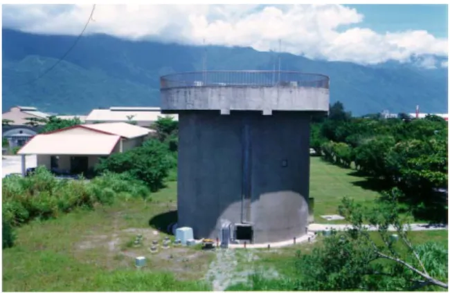
A Large Scale Seismic Test (LSST) had been carried out at Hualien, Taiwan, to investigate the effects of soil-structure interaction during dynamic loadings. It is an in-situ test program sponsored by EPRI and NRC of USA, CEA and EdF of France, TEPCO and CRIEPI of Japan, KINS and KEPCO of Korea and TPC of Taiwan (Tang, 1991). A quarter scale nuclear power plant containment model of diameter 10.82m and height 16.13m, as shown in Figure 1, was built on gravelly deposits for dynamic tests. Two phases of forced vibration tests had been conducted and large amount of earthquake responses had already been recorded.

1

Professor, Department of Civil Engineering, National Taiwan University, Taiwan, Email: chchen2@ntu.edu.tw

2

Figure 1. The 1/4 containment model at Hualien LSST

(a) Surface array (b) Downhole array

Figure 2. Layout of strong motion arrays at Hualien LSST Layout of strong motion arrays

In Hualien Project, an intense strong motion array had been installed around the model structure, as shown in Figure 2. There are three surface linear arrays (designated as ARM1, ARM2 and ARM3, respectively), and three vertical arrays located under the stations A15, A25 and A21 (designated as A15, A25 and A21 vertical arrays, respectively). In each vertical array, four downhole accelerometers were installed at the depths of 5.3 m, 15.8 m, 26.3 m and 52.6 m, respectively. Since A15 and A25 vertical arrays are located at a distance of 52.6 m from the center of the containment model, they can be regarded as free-field arrays. In subsequent analyses, the motions recorded at the A15 vertical array will be adopted for ground motion analysis.

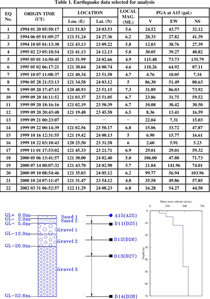
Strong ground motions selected

Since the completion of the LSST arrays at Hualien, a total of 113 earthquakes with local magnitude larger than 4 had been recorded in the period 1993 to 2002. Among them, 22 events will be selected for this study. They are listed as shown in Table 1. Those earthquakes have local magnitudes distributed from 4.6 to 7.3, including the disastrous Chi-Chi earthquake occurred on Sept. 20, 1999 (Event 9). The peak ground accelerations recorded at the surface station A15 are also shown in Table 1. They are distributed from a few gals to 142 gals.

Geological profile at the Hualien LSST site

The Hualien LSST site is located on thick gravelly deposits, namely the Meilung gravel formation. The geological profile near the ground surface is shown in Figure 3 (CRIEPI, 1993). The top 5 meters are loosely deposited sands. Below that, the gravel formation is massive unconsolidated conglomerate composed of pebbles varying in diameter from 10cm to 20cm. The distribution of shear wave velocities obtained from geophysical surveys (P-S logging) is also shown in Figure 3. The velocities increase from 133 m/s at the ground surface to about 550m/s at a depth of 50m.

Table 1. Earthquake data selected for analysis

LOCATION PGA at A15 (gal.)

EQ No.

ORIGIN TIME

(UT) _{Lon. (E) Lat. (N)}

LOCAL MAG. (ML) V EW NS 1 1994 01 20 05:50:17 121 51.83 24 03.53 5.6 24.52 43.77 32.12 2 1994 06 05 01:09:27 121 51.24 24 27.36 6.2 28.33 27.82 41.39 3 1994 10 05 01:13:38 121 43.13 23 09.22 5.8 12.03 38.76 27.39 4 1995 02 23 05:18:54 121 41.13 24 12.13 5.8 30.05 39.27 48.82 5 1995 05 01 14:50:45 121 31.99 24 02.66 4.9 115.48 73.73 135.79 6 1995 05 02 06:17:21 121 38.04 24 00.74 4.6 118.26 64.92 87.11 7 1995 10 07 11:08:37 121 40.34 23 51.58 4.7 4.76 10.05 7.34 8 1996 05 28 21:53:13 121 34.58 24 03.12 5 86.30 51.49 80.63 9 1999 09 20 17:47:15 120 48.93 23 51.15 7.3 31.89 86.03 73.92 10 1999 09 20 18:11:52 121 03.37 23 51.05 6.7 23.86 31.75 59.52 11 1999 09 20 18:16:16 121 02.19 23 50.39 6.7 10.08 30.42 30.50 12 1999 09 20 20:43:48 121 19.48 23 45.58 6.5 8.36 13.41 16.59 13 1999 09 21 00:23:07 － － － 22.04 7.31 15.03 14 1999 09 22 00:14:39 121 02.56 23 50.17 6.8 15.06 33.72 47.87 15 1999 10 16 12:31:55 121 19.42 24 00.13 5 6.90 15.77 16.61 16 1999 10 22 03:10:43 120 25.50 23 31.58 6 2.60 5.91 5.23 17 1999 11 01 17:53:02 121 45.33 23 21.71 6.9 29.01 29.01 59.32 18 2000 05 06 13:41:57 121 30.00 24 02.40 5.0 106.00 47.88 71.73 19 2000 07 14 00:07:32 121 43.70 24 02.90 5.7 21.04 141.96 74.01 20 2000 09 10 08:54:46 121 35.03 24 05.12 6.2 99.77 56.94 103.96 21 2000 10 24 07:11:47 121 31.47 23 54.12 4.8 35.58 49.86 57.85 22 2002 03 31 06:52:57 122 11.29 24 08.23 6.8 16.28 54.27 44.50 0 10 20 30 40 50 60 70 0 250 500 750 Shear wave velocity (m/sec)

De p th ( m )

SPECTRAL ANALYSIS

To investigate the characteristics of ground vibration, the earthquake data recorded from vertical arrays are very useful. The transfer function between the motions recorded at two depths can be used to identify the modal frequencies of vibration of soil layers through spectral analysis.

Transfer functions

Let the accelerogram recorded at certain depth be the i-series and the one on the ground surface be the 1-series. Through the applications of Fourier transforms, one can calculate the spectral ratio by

)

(

)

(

)

(

11 1

f

H

f

H

f

H

ii i

=

(1)

where H_ii( f) and H₁₁(f) are the Fourier transforms of the i- and 1-series, respectively, and H_i1(f)

is the transfer function between i- and 1-series. The transfer function H_i1(f) is a complex-valued

function of frequency. Its absolute value defines the amplitude spectrum, and the arctangent value of the ratio between the imaginary and the real parts defines the phase spectrum. Both of them can be used to identify the modal frequencies of vibration for the soils in between. Usually, the amplitude spectrum is used to identify the modal frequencies. From the first valley of the amplitude spectrum, the predominant frequency can be determined. Furthermore, the predominant frequency can also be

identified from the phase spectrum where the phase angle is equal to 900.

Phase spectrum identification

Theoretically, both the amplitude and phase spectra are continuous smooth function of frequency f. However, the real spectral ratios calculated from earthquake records are highly oscillated in general. In engineering applications, a lot of smoothing techniques have been proposed to smooth the amplitude function in order to identify where the predominant frequency is located. However, the amplitude function smoothed by averaging procedure is still wide-banded at most times and can not easily be used to determine the predominant frequency

.

In this paper, the technique of using phase spectrum to identify the lowest modal frequency will be used as an alternative method. The advantage of using this method is that the curve fitted to the phase

spectrum will across the line of 900 with a very step slope so that the results of identification is not so

sensitive to the method of curve fitting as in the case of using amplitude function. This method has been used by Chen and Chiu(1998). To illustrate the method of predominant frequency identification used in this study, the spectral analysis for the motions of A15 vertical array recorded in the Sept. 20, 1999 earthquake (Event 9) is shown below. Figures 4(a)~(d) are the phase spectra of the transfer functions of D11NS/A15NS, D12NS/A15NS, D13N8/A15NS and D14NS/A15NS, respectively. The frequency interval in those figures is very small (△f=0.0061Hz) so that the data points look rather

scattered. However, they are distributed like a monotonic increasing function starting from about 00

towards 3600. Then, a polynomial of order 9 is used for curve fitting. From the fitted curve as shown

in each figure, the frequency where the fitted curve across the line of 900 is the predominant frequency

of associated soil layers. They are located at frequencies of 8.50Hz, 4.98Hz, 3.45Hz and 2.22 Hz, respectively.

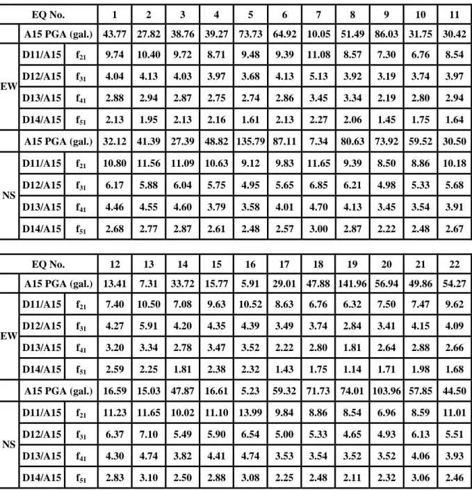
Predominant frequencies

By using the same procedure, the predominant frequencies for all the earthquakes studies are identified as shown in Table 2. In each case, the frequency obtained can be recognized as the predominant frequency of soil layers between the ground surface and the depth when the designated downhole accelerometer located. Therefore, the thicker the soils are, the lower the modal frequency can be identified. It can also be observed from the results obtained, for the same earthquake, the predominant frequencies identified have lower values in the EW direction as compared to the results in the NS direction.

D11/A15 -90 -45 0 45 90 135 180 225 0 1 2 3 4 5 6 7 8 9 10 Frequency (Hz) P h as e ( d eg re e) PHASE FITTED D12/A15 -90 -45 0 45 90 135 180 225 0 1 2 3 4 5 6 7 8 9 10 Frequency (Hz) P h as e ( d eg re e) PHASE FITTED

(a) D11/A15 (b) D12/A15

D13/A15 -90 -45 0 45 90 135 180 225 0 1 2 3 4 5 6 7 8 9 10 Frequency (Hz) P h as e ( d eg ree) PHASE FITTED D14/A15 -90 -45 0 45 90 135 180 225 0 1 2 3 4 5 6 7 8 9 10 Frequency (Hz) Ph ase (d egr ee ) PHASE FITTED (c) D13/A15 (d) D14/A15

Figure 4. Phase spectrum of transfer functions-NS component

D11/A15 0.0 2.0 4.0 6.0 8.0 10.0 12.0 14.0 16.0 0 25 50 75 100 125 150

A15 PGA (gal)

P red omi n an t freq ue ncy (Hz ) _EW NS D12/A15 0.0 1.0 2.0 3.0 4.0 5.0 6.0 7.0 8.0 0 25 50 75 100 125 150

A15 PGA (gal)

P red omi n an t freq ue ncy (Hz ) _EW NS

(a) D11/A15 (b) D12/A15 D13/A15 0.0 1.0 2.0 3.0 4.0 5.0 6.0 7.0 8.0 0 25 50 75 100 125 150

A15 PGA (gal)

P red ominan t f req ue ncy (Hz ) _EW NS D14/A15 0.0 0.5 1.0 1.5 2.0 2.5 3.0 3.5 4.0 0 25 50 75 100 125 150

A15 PGA (gal)

P red ominan t f req ue ncy (Hz ) _EW NS (c) D13/A15 (d) D14/A15

Table 2. Predominant frequencies identified from transfer functions

EQ No. 1 2 3 4 5 6 7 8 9 10 11

A15 PGA (gal.) 43.77 27.82 38.76 39.27 73.73 64.92 10.05 51.49 86.03 31.75 30.42

D11/A15 f21 9.74 10.40 9.72 8.71 9.48 9.39 11.08 8.57 7.30 6.76 8.54

D12/A15 f31 4.04 4.13 4.03 3.97 3.68 4.13 5.13 3.92 3.19 3.74 3.97

D13/A15 f41 2.88 2.94 2.87 2.75 2.74 2.86 3.45 3.34 2.19 2.80 2.94

EW

D14/A15 f51 2.13 1.95 2.13 2.16 1.61 2.13 2.27 2.06 1.45 1.75 1.64

A15 PGA (gal.) 32.12 41.39 27.39 48.82 135.79 87.11 7.34 80.63 73.92 59.52 30.50

D11/A15 f21 10.80 11.56 11.09 10.63 9.12 9.83 11.65 9.39 8.50 8.86 10.18 D12/A15 f31 6.17 5.88 6.04 5.75 4.95 5.65 6.85 6.21 4.98 5.33 5.68 D13/A15 f41 4.46 4.55 4.60 3.79 3.58 4.01 4.70 4.13 3.45 3.54 3.91 NS D14/A15 f51 2.68 2.77 2.87 2.61 2.48 2.57 3.00 2.87 2.22 2.48 2.67 EQ No. 12 13 14 15 16 17 18 19 20 21 22

A15 PGA (gal.) 13.41 7.31 33.72 15.77 5.91 29.01 47.88 141.96 56.94 49.86 54.27

D11/A15 f21 7.40 10.50 7.08 9.63 10.52 8.63 6.76 6.32 7.50 7.47 9.62

D12/A15 f31 4.27 5.91 4.20 4.35 4.39 3.49 3.74 2.84 3.41 4.15 4.09

D13/A15 f41 3.20 3.34 2.78 3.47 3.52 2.22 2.80 1.81 2.64 2.88 2.66

EW

D14/A15 f51 2.59 2.25 1.81 2.38 2.32 1.43 1.75 1.14 1.71 1.98 1.68

A15 PGA (gal.) 16.59 15.03 47.87 16.61 5.23 59.32 71.73 74.01 103.96 57.85 44.50

D11/A15 f21 11.23 11.65 10.02 11.10 13.99 9.84 8.86 8.54 6.96 8.59 11.01

D12/A15 f31 6.37 7.10 5.49 5.90 6.54 5.00 5.33 4.65 4.93 6.13 5.51

D13/A15 f41 4.30 4.74 3.82 4.41 4.74 3.53 3.54 3.52 3.52 4.06 3.93

NS

D14/A15 f51 2.83 3.10 2.50 2.88 3.08 2.25 2.48 2.11 2.32 3.06 2.46

Predominant frequency vs. PGA at A15

The earthquake events selected for analysis have different magnitude of ground shaking. The peak ground accelerations recorded at the surface station A15 are distributed from a few gals to 142 gals. When the predominant frequencies obtained are plotted with respect to the PGA recorded at A15 as shown in Figures 5(a)~(d), it can be clearly seen that the predominant frequency of vibration will decrease with the value of PGA at A15, i.e., with the magnitude of ground shaking. This is due to the effects of nonlinearity of soil when it is subjected to larger shear strains. It can also be observed from those figures, the predominant frequencies identified have lower values in the EW direction as compared to the results in the NS direction. It may be attributed from the effects of soil an-isotropic. The same results had been observed from the results of Forced vibrations performed on the containment of Hualien site (TEPCO, 1993; de Barros, 1995).

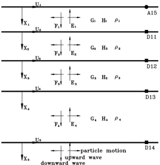
IDENTIFICATION FOR SHEAR WAVE VELOCITY Four layer ground model

In A15 vertical array, the downhole accelerometers are located at depths of 5.3 m, 15.8 m, 26.3 m and 52.6 m, respectively. From the results of geological explorations as shown in Figure 3, it is known that the LSST site has a quite simple geological profile, a sand layer of thickness 5 m overlying a very thick gravel formation. The shear wave velocities shown in this figure are the results measured from the geophysical survey (PS-logging). They are usually regarded as the small strain velocity. Based on that, it is reasonable to adopt a simple ground model, as shown in Figure 6, for wave velocity identification. From ground surface to the depth of 52.6 m, the ground is divided into 4 layers

according to the depths of downhole accelerometers. Each layer has thickness hi and mass density

ρ

_i.

The underlying soils are regarded as a half-space.

The ground motions excited by earthquakes are rather complex in nature. However, for engineering applications, it is often assumed that the horizontal ground motions are mainly produced by vertically propagating SH waves, i.e., the 1-D shear beam model can be applied. By substituting the predominant frequencies identified previously into the characteristic equations of SH wave traveling in the associated soil layers, the shear wave velocity of each layer can then be identified subsequently. It is noted that the damping ratio of soil has very little effect on the modal frequency of ground. Therefore, it is convenient to assume that the damping ratios of soils are all equal to zero in deriving the characteristic equation of soil layers. This leads to a real-valued characteristic equation which is much easier for calculation purpose.

Based on the theory of wave propagation, the characteristic equation of transfer function between different soil layer can be derived as follows.

Single Layer Over a Half-Space

For a single layer on top of an elastic half-space as shown in Figure 7(a), the transfer function can be written as ⎟⎟ ⎠ ⎞ ⎜⎜ ⎝ ⎛ = 1 1 1 2 2 cos s C h f U U

π

(2)

Let f21 be the predominant frequency as identified from the transfer function between the first

downhole station and the surface station, then the equivalent shear wave velocity for the first layer can be estimated by

1 21

1

4

f

h

C

_s

=

(3)

Two Layer Over a Half-Space

For a system of two layers of soil on top of an elastic half-space as shown in Figure 7(b), the transfer function can be written as

⎟⎟ ⎠ ⎞ ⎜⎜ ⎝ ⎛ ⎟⎟ ⎠ ⎞ ⎜⎜ ⎝ ⎛ − ⎟⎟ ⎠ ⎞ ⎜⎜ ⎝ ⎛ ⎟⎟ ⎠ ⎞ ⎜⎜ ⎝ ⎛ = 2 2 1 1 1 1 2 2 1 1 2 2 1 3 2 sin 2 sin 2 cos 2 cos s s s s s s C fh C fh C C fh C fh C U U

_ρ

π

π

_ρ

π

π

(4)

The characteristic equation corresponding to the predominant frequency f31 is

1 1 2 2 2 2 31 1 1 31 _tan 2 2 tan s s s s C C C h f C h f

ρ

ρ

π

π

₌ ⎟⎟ ⎠ ⎞ ⎜⎜ ⎝ ⎛ ⎟⎟ ⎠ ⎞ ⎜⎜ ⎝ ⎛ (5)

Multi-Layer System

For the system of 3 soil layers on top of an elastic half-space as shown in Figure 7(c), the upper two

layers can be regarded as an equivalent uniform single layer of thickness h₁ and velocity C_s1 where

h₁ =h₁+h₂ (6)

Cs1 =4h f1 13. (7)

Now regard the upper three layers of soil as two layers of soil with thicknesses

h

1 and h3 and shear

wave velocities C and C_s1 s3, respectively, as shown in Figure 7(d). Then Cs3 can now be solved based

on Eq.(5) when the predominant frequency f41 is given from Table 2. For a system having more layers

of soil, the same procedure can be used recursively to calculate the shear wave velocity for each layer.

Figure 6. Ground model used for system identification

(a) Single layer model (b) Two layer model

(c) Three layers model (d) Equivalent two layer to system (c)

Table 3. Shear wave velocities for each layer identified EQ No. 1 2 3 4 5 6 7 8 9 10 11 Layer Cs (m/s) Cs (m/s) Cs (m/s) Cs (m/s) Cs (m/s) Cs (m/s) Cs (m/s) Cs (m/s) Cs (m/s) Cs (m/s) Cs (m/s) L1 195 221 206 185 201 199 235 182 155 143 181 L2 263 246 241 240 219 248 310 245 198 241 249 L3 296 329 323 302 321 315 372 441 221 302 315 EW L4 426 448 527 573 348 530 516 436 316 371 333 L1 224 245 235 225 193 208 247 199 180 188 216 L2 394 361 357 356 307 355 433 426 324 353 368 L3 451 556 549 403 408 449 514 407 350 349 394 NS L4 533 606 645 610 583 577 672 647 478 561 596 EQ No. 12 13 14 15 16 17 18 19 20 21 22 Layer Cs (m/s) Cs (m/s) Cs (m/s) Cs (m/s) Cs (m/s) Cs (m/s) Cs (m/s) Cs (m/s) Cs (m/s) Cs (m/s) Cs (m/s) L1 _{157 223 150 204 223 183 143 134 159 158 204} L2 _{279 384 277 271 271 215 241 178 213 268 254} L3 _{346 307 274 405 411 214 302 174 296 292 259} EW L4 _{680 495 391 532 504 308 371 242 370 440 360} L1 _{238 247 212 235 296 209 188 181 148 182 233} L2 _{415 472 354 378 409 317 353 300 351 436 349} L3 _{428 468 388 476 495 364 349 384 364 400 407} NS L4 _{618 674 544 626 664 481 561 442 506 735 523}

Shear wave velocities identified

Based on the procedure described above and the predominant frequencies shown in Table 2, the shear wave velocities for Layer L1(0~5.3m), Layer L2(5.3~15.8m), Layer L3(15.8~26.3m), and Layer L4(26.3~52.6m) can be calculated layer by layer. For all cases, the velocity profile identified from the NS and EW ground responses are summarized in Table 3. It shows that the velocities identified from the EW responses are smaller than those from the NS responses in general. It is as expected because the predominant frequencies obtained from spectral analyses have lower values in EW direction. Gunturi et al.(1998) had used the data of two earthquakes (Events 4 and 5 of this paper) to identify the shear wave velocities of soils by method of cross-correlation function, and similar results to this study were obtained except for the deepest layer.

Shear wave velocity vs. magnitude of ground shaking

To correlate the shear wave velocities with the magnitude of ground shaking, the shear wave velocities identified in Table 3 are plotted with respect to the PGA recorded at the depth of the top of each layer, as shown in Figures 8(a)~(d). It can be clearly seen that the shear wave velocity of each layer is decreased with the value of PGA recorded at the top of each layer, i.e., with the magnitude of ground shaking. This is due to the effect of nonlinearity of soil when it is subjected to larger shear strains. It can also be observed from those figures, the shear wave velocities identified have lower values in the EW direction as compared to the results in the NS direction. It is attributed from the effects of soil an-isotropy. The same trend had been obtained from previous study (Hsu and Chen, 2003).

CONCLUSIONS

Based on the results obtained, some conclusions can be deduced as follows:

1. The method of phase spectrum identification is very effective to deduce the predominant frequency of vibration of soils by using the transfer function of earthquake responses recorded. 2. The predominant frequency of transfer function between the downhole earthquake response and

the ground surface response will decrease with respect to the value of PGA at the ground surface. This is due to the effects of soil nonlinearity when the ground is subjected to larger excitations. 3. For the Hualien site, the shear wave velocity of each layer identified from the earthquake

responses is decreased with respect to the value of PGA recorded at the top of each layer.

4. Both the predominant frequency of transfer functions calculated and the shear wave velocity of soil layers identified from earthquake responses show that the ground of Hualien site is anisotropic in two horizontal directions.

A15~D11 (0m ~ 5.3m) 0 50 100 150 200 250 300 350 0 20 40 60 80 100 120 140 A15 PGA(gal.) Cs ( m /s ) EW NS D11~ D12 (5.3m ~ 15.8m) 0 100 200 300 400 500 600 0 20 40 60 80 100 120 140 D11 PGA(gal.) Cs ( m /s ) EW NS (a) A15~D11 (b) D11~D12 D12~ D13 (15.8m ~ 26.3m) 0 100 200 300 400 500 600 0 20 40 60 80 100 D12 PGA(gal.) Cs (m/s) EW NS D13~ D14 (26.3m ~ 52.6m) 0 150 300 450 600 750 900 0 20 40 60 80 D13 PGA(gal.) Cs (m/s) EW NS (c) D13~D14 (d) D14~D15

Figure 8. Shear wave velocity vs. PGA at the top of each layer

AKNOWLEDGEMENTS

Earthquake data provided by the Taipower company and financial support by the National Science

Council of Taiwan (NSC – 90 - 2811 – E - 002 – 034) are deeply appreciated.

REFERENCES

Chen CH and Chiu HC. “Anisotropic seismic ground responses identified from the Hualien vertical array”, Soil Dynamics and Earthquake Engineering, Vol 17, 371-395, 1998.

Chen CH and Chiu HC. “Identification of shear wave velocity from earthquake ground motions”, Proc., 2nd Inter. Conf. Earthq. Geotech. Engrg., Lisbon, Portugal, 1:205-210, 1999.

Central Research institute of Electric Power industry (CRIEPI). “Soil Investigation Report for Hualien Project”, Report, 1993.