強健性心電信號壓縮演算法之研究

(1)

國立交通大學

電信工程研究所

碩士論文

強健性心電信號壓縮演算法之研究

A Study of Noise-Resilient Compression Algorithm

for ECG Signals

研究生：黎忠孝

指導教授：張文輝博士

(2)

強健性心電信號壓縮演算法之研究

A Study of Noise-Resilient Compression Algorithm

for ECG Signals

研究生：黎忠孝

Student: Trung-Hieu Le

指導教授：張文輝

Advisor: Wen-Whei Chang

國立交通大學

電信工程研究所

碩士論文

A Thesis

Submitted to Institute of Communications Engineering College of Electrical Engineering and Computer Science

NationalChiaoTungUniversity inPartial Fulfillment of the Requirements

for the Degree of Master

in

Communication Engineering

June2013

Hsinchu, Taiwan, Republic of China

(3)

強健性心電信號壓縮演算法之研究

研究生：黎忠孝指導教授：張文輝

國立交通大學

電信工程研究所

摘要

因應高齡化社會的未來趨勢，遠距醫療與居家健康照護已經成為先進國家重點發展的新興服務產業。本論文旨在發展一高效能的心電信號壓縮演算法，以期長時間監測心臟機能的異常徵兆而防患於未然。演算法的設計需兼顧即時製作與強健性能，前者強調簡化運算得以快速實現，後者則要求訊源與量測雜訊能分離處理。第一項研究課題著重於理想傳輸環境下心電訊號壓縮演算法的設計。一維壓縮演算法是採用增益-形狀碼本結構的多層級向量量化機制，另一種是基於國際影像壓縮標準 JPEG2000 的二維壓縮演算法。第二項課題旨在探討能有效對抗環境雜訊干擾的信號除噪技術，其關鍵是參考希伯特-黃轉換理論而設計一兼顧時域及頻域非穩態特性的信號分析技術。針對 MIT-BIH 心電圖資料庫進行的系統模擬結果顯示，新的方法適用於行動心臟照護系統的未來應用。關鍵字：心電信號壓縮，向量量化，小波，信號除噪，希伯特-黃轉換

(4)

A Study of Noise-Resilient Compression Algorithm

for ECG Signals

Student: Le TrungHieu Advisor: Dr. Wen-Whei Chang

Institute of Communications Engineering,

National Chiao Tung University

Hsinchu, Taiwan

Abstract

The volume of ECG data produced by monitoring systems can be quite large, and data compression is needed for efficient transmission over mobile networks. We first propose a new method based on the multiple stage vector quantization in conjunction with gain-shape codebooks. The compression of ECG signals using JPEG2000 is also investigated. The good time-frequency localization properties of wavelets make them especially suitable for ECG compression applications. Also proposed is a method of ECG signal denoising based on Hilbert-Huang transform. This method uses empirical mode decomposition to decompose the signal into several intrinsic mode functions (IMFs) and then the noisy IMFs are removed by using soft-threshold method. Experiments using the MIT-BIH arrhythmia database illustrate that the proposed approach has improved the performance at a high compression ratio.

Keywords: ECG compression, vector quantization, wavelets, signal denosing, Hilbert-Huang transform

(5)

Acknowledgements

Iwould like to acknowledge my advisors, Prof. Wen-Whei Chang, for his valuable guidance throughout my research. I would also like to thank the colleagues in Speech Communication Lab for their helpful suggestions and discussions.

(6)

List of Figures

Figure 2.1 Typical cardiac cycle. ... 5

Figure 2.2 Placements of electrodes ... 7

Figure 2.3 MIT-100 waveform ... 12

Figure 2.6 MIT-118 ... 12

Figure 4.1 The VQ transmission system ... 20

Figure 4.2 VQ-based ECG compression ... 21

Figure 4.3 The gain-shape VQ system ... 22

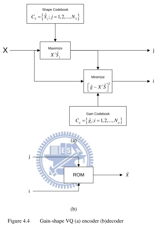
Figure 4.4 Gain-shape VQ (a) encoder (b) decoder ... 25

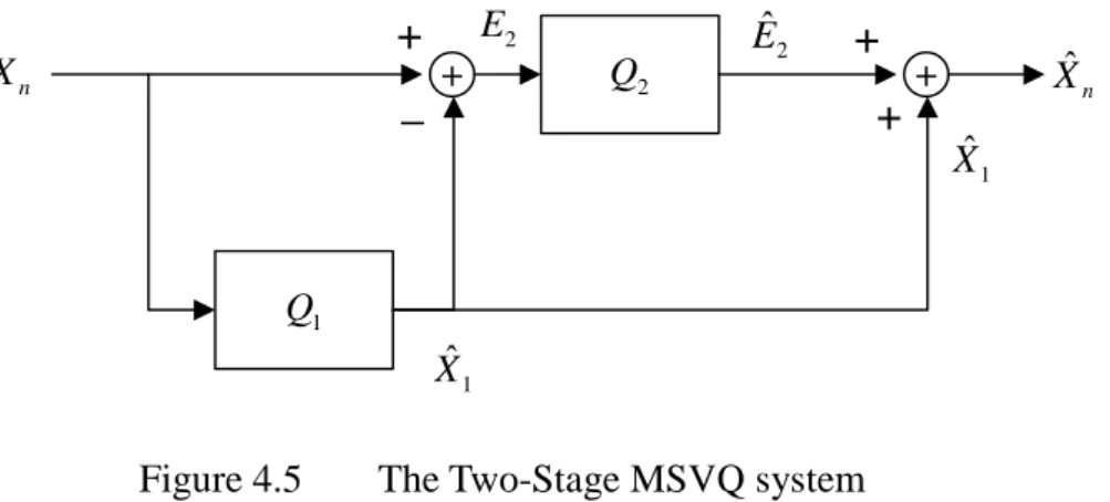
Figure 4.5 The Two-Stage MSVQ system ... 26

Figure 4.6 The proposed ECG compression system: (a) the encoder, (b) the decoder ... 28

Figure 5.1 The block diagrams of JPEG2000 codec ... 30

Figure 5.2 Tiling, DC level shifting and DWT of each image tile component ... 31

Figure 5.3 flow-of-bit view of JPEG2000 encoder ... 32

Figure 5.4 Results obtained by progressive JPEG (P-JPEG), progressive JPEG2000 (both embedded lossless, R, and lossy, NR, versions) and MPEG-4 VTC baseline.[17] ... 33

Figure 5.5 Block diagram of ECG encoder using JPEG2000 ... 34

Figure 5.6 Block diagram of a ECG decoder using JPEG2000 ... 34

Figure 5.7 Detection of ECG cycles ... 35

Figure 5.8 Before period normalization ... 36

Figure 5.9 After period normalization ... 36

Figure 6.1 Results of Algorithm I (k = 8) in MIT-BIH 100: (a) original signal, (b) reconstructed ECG waveforms, and (c) error signals. ... 39

(9)

reconstructed ECG waveforms, and (c) error signals. ... 40

Figure 6.7 MIT-100: (a) Original matrixes, (b) After period-normalization matrixes ... 42

Figure 6.10 MIT-122: (a) Original matrixes, (b) After period-normalization matrixes .... 44

Figure 6.11 Results of Algorithm II in MIT-BIH 100: (a) Original signal, (b) Reconstructed ECG waveforms, and (c) Error signals. ... 44

Figure 6.15 Eight intrinsic mode functions after empirical mode decomposition ... 47

Figure 6.16 Eight intrinsic mode functions after applying soft threshold ... 47

(10)

List of Tables

Table 1.1 World’s top ten causes of death (2008) - WHO ... 1

Table 2.1 Descriptions of waves and durations. ... 6

Table 2.2 Placements of electrodes ... 7

Table 2.3 Beat annotations: ... 10

Table 2.4 Non-beat annotations: ... 11

Table 6.1 Performance results of Algorithm I... 39

(11)

Chapter 1 Introduction

Wireless patient monitoring has been of recent interest to researchers aiming to develop ubiquitous health-care systems able to provide personalized medical treatment continuously and remotely. To realize such systems, physiological signals such as ECG are measured and transmitted wirelessly to the remote server. Due to the limited bandwidth of transmission channel, ECG signal compression methodsare used to reduce the large amount of data.

Every country in the worldis aging with an increase of senior populations. With the increase of the elderly (65 years and over), the health-care issues are becoming more and more significant. Although traditional medical treatments such as face-to-face consultant cannot be replaced, some treatments can be done more efficiently with the biotelemetry. According to Table 1.1, heart diseases account for 12.8% of all deaths in 2008. The ECG is a graphical representation of the electrical activity in the heart and is useful for cardiac disease diagnosis. This motivates the research in designingan ECG monitoring system which can compress and transmit the ECG signals to the hospital or clinical center.

Table 1.1 World’s top ten causes of death (2008) - WHO

World Deaths in millions % of deaths

Ischaemic heart disease 7.25 12.8%

Stroke and other cerebrovascular disease 6.15 10.8%

Lower respiratory infections 3.46 6.1%

Chronic obstructive pulmonary disease 3.28 5.8%

Diarrhoeal diseases 2.46 4.3%

HIV/AIDS 1.78 3.1%

Trachea, bronchus, lung cancers 1.39 2.4%

Tuberculosis 1.34 2.4%

Diabetes mellitus 1.26 2.2%

Road traffic accidents 1.21 2.1%

(12)

transmission capacity. This thesis first applies theHilbert-Huang Transform as a method to ECG signaldenoising.One dimensional ECG compression is achieved by using theMultistage Vector quantization (MSVQ) together with Gain-shape codebooks. Also proposed is a compression scheme based on JPEG2000, a well-established standard for compression of still images.

ECG signalsare often corruptedby some noise during the measurement. The main interferences include baseline drift, electromyography, interference and frequency interference. Since ECG is very weak compared tonoise, digital signal processing methods used for signal denoisingarenecessary. Previous research suggests the use of Hilbert-Huang Tranform for noise filtering and denoising. The empirical mode decomposition (EMD) and the associated Hilbert transform, together designated as the Hilbert-Huang Transformation (HHT), are discussed in this work. The expansion of ECG data via the EMD method only has only a limited number of intrinsic mode functions(IMFs). Since the smaller scale IMFs can be considered as noise-dominated components, soft-threshold denoising methods can be used to remove the most noisy IMFs.

Most of the existing ECG compression methods adopt one-dimensional (1-D) representations for ECG signals, including direct waveform coding, transform coding, and parameter extraction methods. However, since the ECG signals have both sample-to-sample (intra-beat) and beat-to-beat (inter-beat) correlation, some 2-D compression techniques have been proposed for higher compression ratios [27,28]. These methods start with a preprocess procedure that converts 1-D to 2-D representations through the combined use of QRS detection and period normalization. Afterwards, the conventional image codec such as the JPEG standard can be used to compress these resulting 2-D arrays. JPEG2000 is the latest international standard for compression of still images. Although the JPEG2000 codec is designed to compress images, we illustrate that it can also be used to compress other signals.

(13)

In this thesis, we illustrate how the JPEG2000 codec can be used to compress electrocardiogram (ECG) data. In addition, this workalso proposes a method based on multiple stage vector quantization (MSVQ) in conjunction with gain-shape codebook structure.We will evaluate the performances of the proposed schemes by using the ECG records from the MIT-BIH arrhythmia database.

This thesis is organized as follows. In Chapter 2, the fundamental of ECG signal will be reviewed, including the characteristic of ECG and the MIT-BIH database. Chapter 3 introduces the HHT algorithm and using HHT for denoising. Chapter 4 represents VQ-based compression, including GSVQ and MSVQ. Chapter 5is derived by using JPEG2000 compression codec on ECGsignals. Chapter 6 and Chapter 7 givesthe results of experiments and conclusion.

(14)

Chapter 2 Fundamental of ECG Signals

Electrocardiography(ECG) is a transthoracic (across the thorax or chest) interpretation of the electrical activity of the heart over a period of time, as detected by electrodes attached to the surface of the skin and recorded by a device external to the body. The recording produced by this noninvasive procedure is termed an ECG. ECG is commonly used to measurethe rate and regularity of heartbeats, as well as the size and position of the chambers, the presence of any damage to the heart, and the effects of drugs or devices used to regulate the heart, such as a pacemaker. The ECG sources used in this research are acquired by using an open MIT-BIH database.In this chapter, introduction of ECG measurement and the ECG MIT-BIH sources used in our workare discussed.

2.1 ECGcharacteristic

Goal of an ECG device is to detect, amplify, and record the electrical changes caused bydepolarization and repolarization of heart muscle. Each heart muscle cell, at rest condition, has a negative charge across its cell membrane and is called polarized. The negative charge can be increased to zero, and the phenomenon of depolarization causes the heart to contract. Afterwards, the heart muscle cell will be recharged, called repolarization, which makes the heart to expand. A cardiac cycle begins when the sinoatrial node (SA) generates the impulse, which will run through the heart. The conducting system of the heart can be summarized as follows:

1. The impulse generated from SA node will signal the muscle in the atria to beat, resulting in contraction,during which the blood is pushed from atria into ventricles. 2. The impulse propagates to atrioventricular(AV) node and then delays for about 1

(15)

3. The impulse propagates to the ventricles through the right bundle branch (RBB), the left bundle branch (LBB), and other nerves. Thisresultsin the ventricular contraction, during which the blood is pushed to the body.

4. The muscle cells are recharged (repolarization) and it expands the atrial so that the blood is allowed to return to the heart. Then, the next heartbeat repeats.

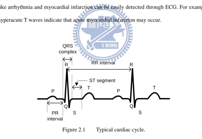
A typical cardiac cycle (ECG cycle) is composed of a P wave, a QRS complex, and a T wave. In addition, there are U wave and J wave within an ECG cycle, but their amplitudesare so low that they are often ignored. Different types of wave reflect the different stages of the heartbeats. A detailed description of each wave and its duration are shown in Fig2.1and Table2.1. ECG is the most important tool to diagnose any damage to the heart. Symptoms like arrhythmia and myocardial infarction can be easily detected through ECG. For example, hyperacute T waves indicate that acute myocardial infarction may occur.

PR interval S Q P R T ST segment QRS complex RR interval S Q P T R

(16)

Table 2.1 Descriptions of waves and durations.

Name Descriptions Duration

P wave Represents theatrial depolarization. Shorter than 0.12 seconds PR interval The interval between the points of the P

wave to Q wave.

Longer than 0.12 seconds and shorter than 0.2 seconds. QRS complex Represents the ventricular depolarization

and atrial repolarization.

Longer than 0.08 seconds and shorter than 0.12 seconds. ST segment The period during which the ventricles are

depolarized.

Longer than 0.08 seconds and shorter than 0.12 seconds T wave The last wave of a normal cardiac cycle,

representing the ventricular repolarization. Shorter than 0.16 seconds RR interval The interval between two R waves. Longer than 0.6 seconds and

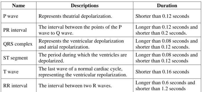
shorter than 1.2 seconds While the heartbeats are caused by a series of electrical activities in the heart, we can collect and record these signals by attaching electrodes on the surface of the skin. When measuring ECG, usually more than two electrodes are used and they can be combined into a pair whose output is called a lead. The most common clinically-used one is 12-lead ECG where ten electrodes are used. Each electrode has a specific label (name), including RA, LA, RL, LL, V1, V2, V3, V4, V5, and V6. The placements and labels of electrodes are illustrated inFig2.2 andTable 2.2, respectively.

(17)

RA

LA

RL

LL

(a)

(b)

Figure 2.2 Placements of electrodes

Table 2.2 Placements of electrodes

Electrodes’ label Placement

RA _{On the right arm.} LA _{On the left arm.} RL _{On the right leg.} LL _{On the left leg.}

V1 _{In the space, between rib 4 and rib 5, to the right side of the breastbone.} V2 _{In the space, between rib 4 and rib 5, to the left side of the breastbone.} V3 _{In the place between lead V2 and lead V4.}

V4 In the space between rib 5 and rib 6, and on an imaginary line extended from the collarbone’s midpoint.

V5 _{In the place between lead V4 and lead V6.}

V6 In the space horizontally even with lead V4 and V5, and on an imaginary line extended from the middle of the armpit.

(18)

The twelve leads contain sixprecordial leads (V1~V6) in the horizontal plane, three standard limb leads (I, II, III), and three augmented limb leads (aVR, aVL, aVF) in the frontal plane.The twelve leads can also be divided into two types: bipolar and unipolar. While the former has one positive and one negative pole, the latter has two poles with the negative onemade of signals from many other electrodes. For example, leads I, II, and III are bipolar leads, while others are unipolar leads. Thedefinitions of twelve leads are given as below.

1. Lead aVR: the positive electrode is on the right arm and the negative one is a combination of two electrodes on the left arm and left leg.

( ) / 2

RA LA LL

Lead aVRV  V V (2.1)

2. LeadaVL: the positive electrode is on the left arm and the negative one is a combination of two electrodes on the right arm and left leg.

( ) / 2

LA RA LL

Lead aVLV  V V (2.2)

3. Lead aVF: the positive electrode is on the leftleg and the negative one is a combination of two electrodes on the left arm and right arm.

( ) / 2

LL LA RA

Lead aVFV  V V (2.3)

4. Lead I: the positive electrode is on the leftarm and the negative one is on the right arm.

( _LA _RA)

Lead I  V V (2.4)

5. Lead II: the positive electrode is on the leftleg and the negative one is on the right arm.

( _LL _RA)

Lead II V V (2.5)

6. Lead III: the positive electrode is on the leftleg and the negative one is on the left arm.

( LL LA)

(19)

Of the 12 leads in total, each records the electrical activity of the heart from a different perspective, which also correlates to different anatomical areas of the heart for the purpose of identifying acute coronary ischemia or injury. Two leads that look at neighbouring anatomical areas of the heart are said to be contiguous. The relevance of this is in determining whether an abnormality on the ECG is likely to represent true disease or a spurious finding.

Modern ECG monitors offer multiple filters for signal processing. The most common settings are monitor mode and diagnostic mode. In monitor mode, the low-frequency filter is set at either 0.5Hz or 1Hz and the high-frequency filter is set at 40Hz. This limits artifacts for routine cardiac rhythm monitoring. The high-pass filter helps reduce wandering baseline and the low-pass filter helps reduce 50- or 60-Hz power line noise.

2.2 MIT-BIHECGdatabase

The MIT-BIH Arrhythmia Database was the first generally available set of standard test material for evaluation of arrhythmia detectors, and it has been used for that purpose as well as for basic research into cardiac dynamics at about 500 sites worldwide since 1980. Together with the American Heart Association (AHA) Database, it played an interesting role for evaluating automated arrhythmia analysis in research community. The ECG recordings came from the Beth Israel Deaconess Medical Center and were further digitized and annotated by a group at Massachusetts Institute of Technology. The database contains a total of 48 half-hour data, two-channel, 24-hour, obtainedfrom 47 subjects.The subjects included 25men aged 32 to 89 years and 22 womenaged 23 to 89 years; approximately 60%of the subjects were inpatients.One channel is a modified limb II (MLII), and the other is usually V1 but can be V2, V4, or V5. The sample rate is 360Hz and each sample point is scalar quantized into 11 bits.

(20)

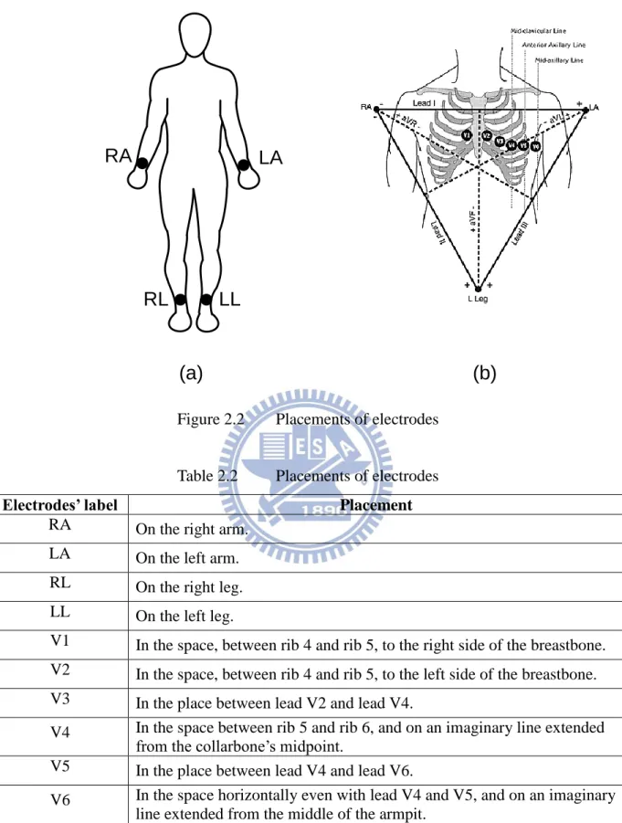
at those locations. The annotators were instructed to useall evidence available from both signals toidentify every detectable QRS complex. For example, many of the recordings that contain ECG signals have annotations that indicate the times of occurrence and types of each individual heart beat. The standard set of annotation codes was originally defined for ECGs, and includes both beat annotations and non-beat annotations. Most MIT-BIH databases use these codes(annotation) as described below.

Table 2.3 Beat annotations:

Code Description

N Normal beat (displayed as "·")

L Left bundle branch block beat

R Right bundle branch block beat

B Bundle branch block beat (unspecified)

A Atrial premature beat

a Aberrated atrial premature beat

J Nodal (junctional) premature beat

S Supraventricular premature or ectopic beat (atrial or nodal)

V Premature ventricular contraction

r R-on-T premature ventricular contraction

F Fusion of ventricular and normal beat

e Atrial escape beat

j Nodal (junctional) escape beat

n Supraventricular escape beat (atrial or nodal)

E Ventricular escape beat

/ Paced beat

f Fusion of paced and normal beat

Q Unclassifiable beat

(21)

Table 2.4 Non-beat annotations:

Code Description

[ Start of ventricular flutter/fibrillation ! Ventricular flutter wave

] End of ventricular flutter/fibrillation x Non-conducted P-wave (blocked APC)

( Waveform onset ) Waveform end p Peak of P-wave t Peak of T-wave u Peak of U-wave ` PQ junction ' J-point

^ (Non-captured) pacemaker artifact | Isolated QRS-like artifact

~ Change in signal quality

+ Rhythm change s ST segment change T T-wave change * Systole D Diastole = Measurement annotation “ Comment annotation

@ Link to external data

As shown in Fig 2.3, “A” and“”represent atrial premature beat and normal beats and can be seen in MIT-100.

(22)

Figure 2.3 MIT-100 waveform

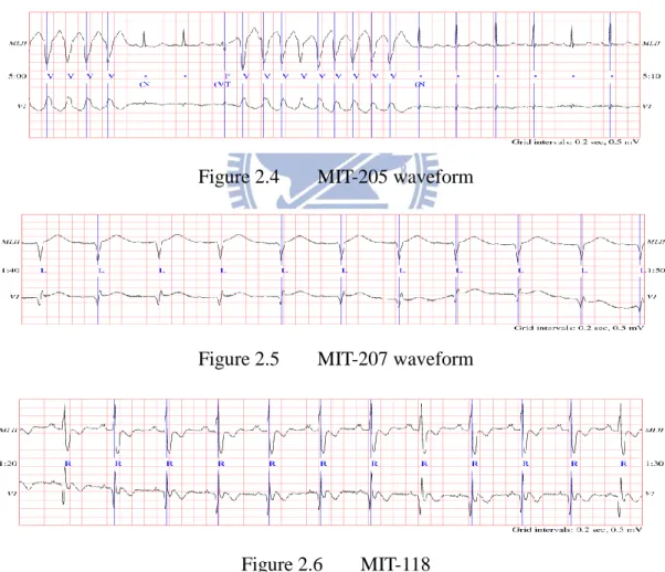
As shown in Fig 2.4 – Fig 2.6, several annotations are combined in MIT 205 with “F” and “V”, or with only specific annotation such as “L” inMIT-207 and “R” in MIT-118.

(23)

Chapter 3 Hilbert-Huang Transform for ECG Denoising

ECG signals are very weak compared to the measurement noise, so that some analysis tools are needed for signal denoising. Hilbert-Huang Transform (HHT) has become a powerful tool for signal analysis, since its introduction in 1996. This is due to its ability to extract periodic components which are embedded in a certain signal. This chapter briefly introduces HHT and its aplications to ECG signal denoising, especially on high frequencies denoising.

3.1 Hilbert-Huang Transform

Traditional data analysis methods are derived by assuming that the signals are linear and stationary. In recent years some new methods have been proposed which apply an adaptive basis to analyze nonstationary and nonlinear data. Among them, HHT seems to be a good approach which matches all the requirements.

The HHT consists of two parts: empirical mode decomposition (EMD) followed by Hilbert spectral analysis (HAS). For nonlinearand nonstationary data,this method provides a powerful analysis, especially for time-frequency analysis and energy representations. In addition, theHHT displays the physical meanings of signals under investigation. The power of the method is verified by experiment and its applications have been widely studied.

3.1.1 Empirical mode decomposition (EMD)

As discussed by Huang et al[20], EMD is the first step to deal with data from nonstationary and nonlinear processes. The decomposition is based on the simple assumption that any data is composed of different intrinsic modes functions (IMF). Each IMF, linear or nonlinear, represents a simple oscillation, which has the same number of extrema and zero-crossings. At any given time, the data may have many different coexisting modes of

(24)

the following two conditions:

(1) In the whole data set, an IMF with the number of zero and extreme crossings must equal or differ at most by one

(2) At the random time, the mean value of two envelopes which are defined by the local maximum and local minimum need to be zero. On the time axis, this implies that the envelopes are symmetric.

With the definition of the IMF, we can observe that IMF is typical of an oscillatory mode. The IMF not only represents constant amplitude and frequency, as each harmonic component does, but also has a variable amplitude and frequency as functions of time.

The procedure of producing IMFs starts with finding local maximum and minimum of the signal. The up and down of the signal are calculated by cubic spline interpolation. The average value of the curve’s maxima and minima is called m with relation to ₁ x t( ) as:

 

1 1

( )

x t m t h t (3.1)

The first component h is checked to see if it satisfies the above-mentioned two conditions. If ₁ not satisfied, we treat h as original data and repeat the above process to obtain 1

1( ) 11( ) 11( ) h t m t h t

(3.2) This calculation is repeated till we find out h , _1k

 

1

 

1

 

1k 1 k k

h _ t m t h t (3.3)

which satisfies the two conditions and is designed as the first IMF c t₁

 

h_1k

 

t . It means c ₁ should contain the shortest periodic component of the signal.

After taking c out of the original data, we have the residue, ₁

 

1 1

( )

x t c t R t (3.4)

(25)

new data followed by the filtering process. This procedure is repeated with all R i

 

1 2 2 ,..., n 1 n n

R t c t R t R_ t c t R t (3.5)

The process can be stopped when R t becomes so small that no more IMFs can be _n

 

extracted or when R becomes a single function. By summing up the IMFs, the _n x t( ) can be represented by:

 

1 ( ) n i n i x t c t R t  



 (3.6)

By decomposing a data into n-empirical modes, the whole EMD can be considered as the mean trend or the scale processing with each IMF representing the characteristics of each scale. In other words, the IMF eliminates the nonstationary character of the original signal.

3.1.2 Hilbert Transform

Having obtained the IMF components, the Hilbert transform process is performed on every IMF to obtain a new time series y t in the transform domain as follow _i( )

1 ( ') ( ) ' ' i i c t y t p dt t t   



(3.7)

With this definition, a complex series ( )z t is formed in terms of _i ( )

( ) ( ) ( ) ( ) j t

i i i i i

z t c t  jy t a t e  (3.8)

where the amplitude of ( )z t will be: _i

2 2 ( ) ( ) ( ) i i i a t  c t y t (3.9) and phase ( ) ( ) arctan ( ) i i i y t t c t   _ _   (3.10)

(26)

( ) ( ) i i d t t dt   _{ } _   (3.11)

Unlike the FFT, a t and _i

 

_i

 

t derived by HHT are functions of time t, so the HHT can characterize the variation of power with time.

3.2 HHT-based denoising

After EMD on the noisy signal are conducted, the energy of the IMFs is analyzed to separate the IMF components into signal-dominated parts and noise-dominated parts. By exploiting the fact that the scale of the IMFs components is dramatically increasing, the energy of IMFs of Gauusian white noise will reduce as the number of decomposition increases. With this approach, the denoising processing based on HHT will be performed by applying filtering on each IMF.

A.

Energy analysis

Following the work of [24-25] the energy of x t( ) can be represented as

 

2 T t i E a t  



(3.12)

According to the observation of N.E.Huang [20], when the energy approaches the lowest point, this point is considered as the boundary between the most noisy part and signal part. When the energy of IMF lower than i IMFi1, IMF is considered to be the boundary. i

B.

Soft-threshold denoising process

Soft-threshold denoising method is proposedby Donohoet. al.[21-23].Each IMF component dominated by the Gaussian white noise must carry out soft-thresholddenoising process, and the corresponding threshold is

 

2 log

i i

thr  N (3.13)

where N is the length of each IMF. 2

i

(27)

the equation i MADi/ 0.6745. MAD is the absoluate median deviation of the i-th layer i i IMF













i i i

MAD median abs IMF median IMF (3.14)

After all IMFs are applied with soft-threshold denoising process, we reconstruct the denoised signal by overlaying the EMD.

(28)

Chapter 4 VQ-based ECG Compression

Vector quantization (VQ) is a lossy data compression method based on the principle of block coding. It is a fixed-to-fixed length algorithm. In the earlier days, the design of a vector quantizer (VQ) is considered to be a challenging problem due to the need for multi-dimensional integration. In 1980, Linde, Buzo, and Gray (LBG) proposed a VQ codebook construction algorithm based on a training sequence, which bypasses the need for multi-dimensional integration.

4.1 Vector Quantization

Extensive studies of vector quantizers or multidimensionalquantizershave long been performed by many researchers [1-5]. The design of optimal vector quantizers fromempirical data were proposed byLinde, Buzo, and Gray [6] using a clustering approach. This algorithm is now commonlyreferred to as the LBG algorithm. A vector quantizer can bedefined as a mapping Q of K-dimensional Euclidean space

R

kinto a finite subset Yof

R

k. Thus,

: K

Q R Y (4.1)

whereY 



x ii; 1, 2,...,N



is a set of N reproductionvectors.As shown in Fig 4.1, the VQ can

also be seenas a combination of two functions: an encoder, which representsthe input vector xwith an index of the reproductionvector specified by Q x

 

, and a decoder, which uses thisindex to generate the reproduction vector ˆx . Thebest mapping Qis the one which _i minimizes a distortionmeasure d x x



,



which represents the penalty or costassociated with

reproducing vectors xby x. TheLBG algorithm and other variations of this algorithm are

derived basedupon this minimization, using a training set as the signal.

One simple distortion measure for waveform coding is thesquare error distortion given by

(29)

 

2 1



2



0 , K j j j d x x x x x x     



 (4.2)

A weighted mean square error (WMSE) distortion can also be used [7]. Other error distortion measures have also beensuggested, but they are too expensive computationally forpractical implementation. One problem with vector quantizationis that the encoder needs to searchthe whole codebook in order to identify the nearest vector template matchingto an input vector.

The most important part which cosumes the most time is VQ codebook design.The goal in designing an optimal vector quantizer is toobtain a codebook consisting of N reproduction vectors, suchthat it minimizes the expected distortion. Optimality is said tobe achieved if there is no other quantizer that can achieve theminimum expected distortion. Lloyd [8] proposed an iterativenonvariational technique known as his “Method I” for thedesign of scalar quantizers. Linde et al [9]. extendedLloyds’ basic approach to the general case of vector quantizers.

Let the expected distortion be approximated by the time-averagedsquare error distortion given by

 





1





0 1 , , N i i i D x q x d x x N   



(4.3)

The LBG algorithm for an unknown distribution training sequenceis given as follows

1) Let N = number of levels; distortion threshold  0.Assume an initial N level reproduction alphabet Aˆ₀, and atraining sequence



x jj; 0,1,...,n1



, and m = number of

iterations, set to zero.

2) Given Aˆm 



y ii; 1,...,N



, find the minimumdistortion partition

 

ˆ



_; _1,...,



m i

(30)

 









1





0 ˆ _, ˆ ₁ _min _, m n m m m j y A j D D A P A n d x y       _ _ 



(4.4)

3) If



Dm₁Dm



/Dm, stop the iteration and useAˆm asthe final reproduction alphabet;

otherwise continue.

4) Find the optimal reproduction alphabet x P Aˆ



 

ˆ_m







x Sˆ

 

_i ;i1,...,N



for P A

 

ˆm

where

 

: 1 ˆ j i m i j j x S i x S x S  



(4.5)

5) Set

A

ˆ

_m_₁



x S

ˆ

 

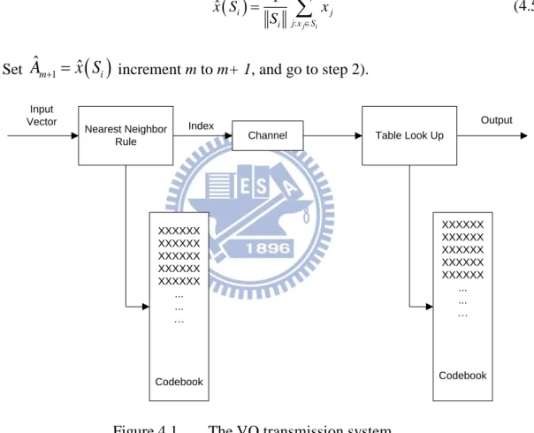
_i increment m to m+ 1, and go to step 2).

Nearest Neighbor

Rule Channel Table Look Up

XXXXXX XXXXXX XXXXXX XXXXXX XXXXXX ... ... … Codebook XXXXXX XXXXXX XXXXXX XXXXXX XXXXXX ... ... … Codebook Input

Vector _Index Output

Figure 4.1 The VQ transmission system

In the above iterative algorithm an initial reproductionalphabet Aˆ₀ was assumed in order to start the algorithm. Thereare a number of techniques to construct the initial codebook. Thesimplest technique is to use the first widely spaced words fromthe training sequence. Linde et al. [9] used a splittingtechnique where the centroid for the training sequence wascalculated and split into two close vectors. The centroids or thereproduction vectors for the two partitions were then calculated.Each resulting vector was then split into two vectors

(31)

andthe above procedure was repeated until an N-level initialreproduction vector was created. Splitting was performed byadding a fixed perturbation vector



to each vector y_j producing two vectors y_j and y_j .

4.2 VQ for ECG Compression

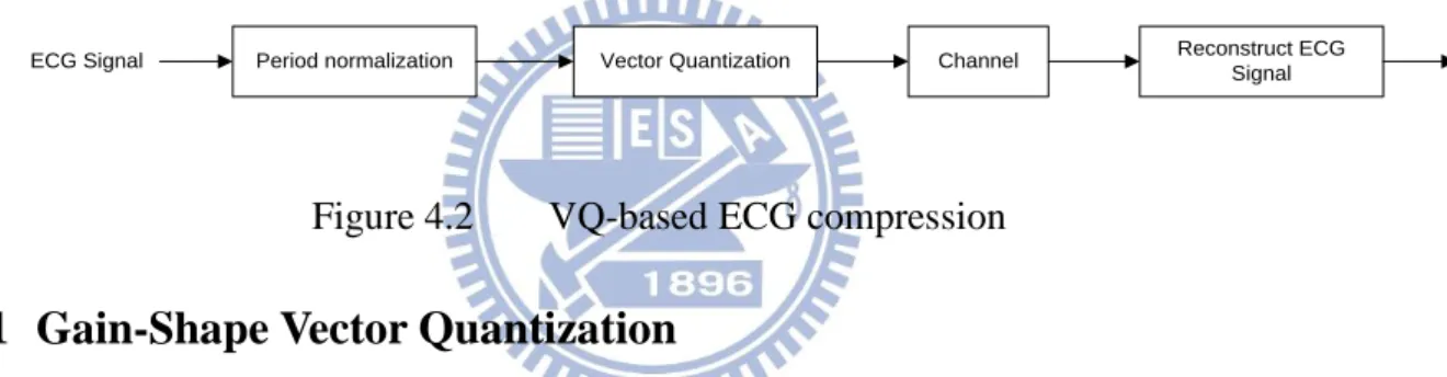
The lengths of heart-beat segmentsare different so each ECG cycle has to be normalized to a fixed length. A predefined length is obtained by calculating the average length of a large training set of ECG cycles. Cubic spline interpolation is then used due to the simplicity of construction, and accuracy of evaluation. The block diagram of VQ-based ECG compression is shown in Fig 4.2.

Period normalization Vector Quantization Channel Reconstruct ECG _Signal ECG Signal

Figure 4.2 VQ-based ECG compression

4.2.1 Gain-Shape Vector Quantization

Although conventional VQ works well for its high compression ratio and high qualityreconstruction, there exist many variants for different applications.Theconventional VQ encoder requires computational complexity proportional to

k

2

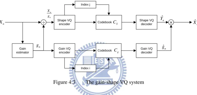
M , which implies that itscomplexity grows exponentially. A large codebook is needed to achieve reasonable performance if the dynamic range of the input vector is large, since there should be more codewords to represent original input vectors. Therefore a good performance of VQ is reached at the cost of high encoding complexity due to the use of a large codebook. To solve this problem, gain-shapeVQ(GSVQ) is used in this thesis. GSVQ is a technique that decomposes reproduction vector into a scalar gain and a shape vector, which is normalized by

(32)

serves as a normalizing scale factor. The normalized input vector is called the shape. Thebasic idea of GSVQ is that the same pattern of variation in a vector may recur with a wide variety of gain values. It suggests that the probability distribution of the shape is approximately independent of the gain. We would then expect very little compromise in optimality with a product code structure. Viewing from another perspective, we can say that the code is permitted to handle the dynamic range of the vector separately from the shape of the vector. GSVQ was introduced in [10] and optimized in [11].

Gain estimator Shape VQ encoder Gain VQ encoder Shape VQ decoder Gain VQ decoder ÷ × n X Xˆ_n n n X g n g _ˆ n g ˆ n Y Codebook Codebook Index j Index i S C g C

Figure 4.3 The gain-shape VQ system

In Gain-shape VQ, the gain g is the norm of a k-dimensional input vector _n X , _n

1 2 2 1 k n n ni i g X x     _{ } _ 



 (4.6)

and shape S refers to the normalized input vector, that is, n

n n n

S  X g (4.7)

All the shape vectors in the shape codebook Cs have unit gain. With this product code decomposition, the shape vector lies on the surface of a hypersphere in k-dimensional space and is therefore easier to quantize than the original vector X. In order to determine the optimal encoding structure, we begin by examiningthe performance criteria. Here we assume the squared errordistortion measure

(33)



_ˆ



_ˆ 2

ˆ ˆ

,

d X gS  X gS (4.8)

where

ˆg

is the quantized version of g and ˆS is the quantized version of theshape S. The gain and shape codebooks are denoted by Cg and Cswith sizes Ng and Ns, respectively. Expanding this expression gives



_ˆˆ



2 _ˆ2 _ˆ

 

ˆ

, 2 t

d X gS  X g  g X S (4.9)

This distortion can be minimized over

ˆg

and ˆS in two steps. First select the shape vector S which minimizes the third term, that is, pick the ˆS that maximizes X Stˆ. Note that

ˆg

is always positive and its value does not influence the choice of ˆS. It is also important to note that the input vector need not be itself gain normalized in order to choose the best shape vector. Such normalization would involve division by the input gain and would significantly increase the encoder complexity. The maximum correlation selection obviates any such computation. Once the shape codeword is chosen, select the

ˆg

to minimize the resulting function of

ˆg

, thus

 



 



2

 

2

2 ₂ ˆ 2 ˆ ˆ

ˆ 2ˆ t ˆ t ˆ t

X g  g X S  X  g X S g X S (4.10)

which is accomplished by chosing

ˆg

to minimize 2 ˆ ˆ t g X S      (4.11)

for the previously chosen (unit norm) S. Note that the second step requires only a standard scalar quantization operation, where the gain nearest to the quantity X S is selected fromthe tˆ gain codebook.

The optimal encoding rule is a two-step procedure, where the first step involves a single feature (the shape) and one codebook. The second step depends on the first step in its

(34)

effect, the first step affects the distortion measure used to compute the second step. Note that this is the reverse of the mean-removed VQ where the scalar parameter is quantized followed by the residual (corresponding to the shape) quantized. This procedure can also be seen to yield the optimal (nearest neighbor) product codeword by observing that

 



2





2

 



ˆ,ˆ ˆ ˆ

ˆ ˆ

ˆ ˆ ˆ ˆ

min 2 t min 2 max t

g

S g g  g X S  g  g S X S (4.12)

Both the encoder and decoder of the gain-shapequantizerare shown in Fig 4.4 and 4.5

We next consider the task of codebook design for gain-shape VQ. We begin with a training setT of input vectors, x , each of which realizes the random vector X. The _i objectiveis to find the shape and gain codebooks that minimize the averagedistortion incurred in encoding the training vectors. There are several variations of the Lloyd algorithm by whichthis task can be accomplished [11], but we focus on the basic onewith good properties. A Gain-shape VQ is completely described by three objects:

 The gain codebookC_g 



g iˆ ;_i 1,2,...,N_g



,

 The shape codebook C_S 



Sˆ ;_j j1, 2,...,N_S



, and

 A partition R



R_{i j}_, ;i1, 2,...,N_g; j1, 2,...,N_s



ofN_gN_s cells describing the encoder, that is, if xR_{i j}_, , then x is mapped into (i,j) and the resulting reproduction is formed from the shape-gain vector



g Sˆ ,_i ˆ_j



. We express this as

 

ˆ_i

(35)

Shape Codebook Maximize Minimize Gain Codebook



ˆ ; 1, 2,...,



S j S C  S j N ˆ t j X S 2 ˆ ˆ t g X S     



ˆ ; 1, 2,...,



g i g C  g i N

X

j i (a) j i ROM Xˆ (b)

Figure 4.4 Gain-shape VQ (a) encoder (b)decoder

4.2.2 Multistage VQ

In some cases, ECG signals have a wide variation of gain or of mean values, then shape-gain or mean-removed VQ methods are not likely to be very helpful. This motivates own research into ECG compression using other variants of VQ. If the dimension is quite large, partitioned VQ would certainly solve the complexity problem but might severely degrade

(36)

structured VQ and classified VQ are not helpful. Furthermore, transform VQ may be of limited use if the degree of achievable compaction still results in a high vector dimension.

One alternative technique that has proved valuable in speech and image coding applications is the multistage or cascaded VQ [12]. The basic idea of multistage VQ (MSVQ) is to divide the encoding task into successive stages, where the first stage performs a coarse quantization of the input vector using a small codebook. Then, a second stage quantizer operates on the error vector between the original and first stagequantizer’s output. The quantized error vector provides a second approximation to the original input vector, thereby leading to a refined representation of the input. We first consider the special case of two-stage VQ as illustrated in Fig 4.5. The input vector X is quantized by first stage vector quantizer denoted byQ . The quantized approximation 1 Xˆ1 is then subtracted from Xto produce the error vector E . This error vector is then applied to a second vector quantizer₂ Q , yielding ₂ the quantized outputEˆ₂. The overall approximation

ˆX

to the input X is formed by summing the first and second approximations, Xˆ₁and Eˆ₂ . The encoder for this MSVQ scheme transmits a pair of indexes specifying the selected code vectors for each stage.The decoder performs two table lookups and then sums the two code vectors.

+ n X Xˆ_n 1 Q 2 Q

+

_ 2 E 1 ˆ X 2 ˆ E 1 ˆ X

Figure 4.5 The Two-Stage MSVQ system

By inspection of the figure it may be seen that the input-output error isequal to the quantization error introduced by the second stage, XXˆ E₂Eˆ₂. From this equation it

(37)

can be readily seen that the signal toquantizing noise power ratio in dB (SNR) for the two stage quantizer isgiven by SNR  SNR₁  SNR₂, where SNR is the SNR for the i-_i thquantizer. In comparison with a single quantizer with thesame total number of bits, a two-stage quantizer has the advantage that thecodebook size of each two-stage is considerably reduced so that both the storagerequirement and the search complexity are substantially lowered. Theprice paid for this advantage is an inevitable reduction in the overall SNRachieved with two stages.The general MSVQ method can be generalized by induction fromthe two-stage scheme. By replacing the box labeled Q in Fig4.5, witha two-stage VQ structure, we obtain ₂ 3-stage VQ. By replacing the last stageof an m-stage structure, we increase the number of stages to m + 1.

An ECG compression technique is suggested in this thesis thattakes into consideration both dynamic range of the input vector, as well as light complexity of the reconstruction. In practice, multistage coders oftenhave only two and occasionally three stages. As far as we know, there hasbeen no report of a coding system using four or more stages.In our work, the dynamic range isreduced by using Gain-shape VQas the first stage. The second stage quantizeristhen used toquantize the first stage error vector to provide a further refinement as shown in Fig 4.6.The encoder transmits indexes I I I to the decoder, which then performs 1, 2, 3 a table-lookup in the respective codebooks and forms the multiply and sum as Fig 3.8. The

complexity is reduced from

1 1 m m i i i i N N N  









. Thus both the complexity and storage requirementscan be greatly reduced using multistage GSVQ.

(38)

Gain estimator Gain’s VQ encoder Gain’s VQ decoder Shape’s VQ encoder Shape’s VQ decoder ÷ X n X n n X g n g ˆ n Y +   VQ encoder ˆ_n g ˆ n Y  Index I1 Index I3 Index I2 (a) Index I1 Index I3 Index I2 Shape’s VQ decoder Gain’s VQ decoder VQ encoder X + ˆ_n g ˆ n X ˆ n Y ˆ n Y  (b)

(39)

Chapter 5 JPEG2000-Based ECG Compression

With the increasing use of multimedia technologies, image compression requires higher performance as well as new features. To address this need in the specific area of still image encoding, a new standard the JPEG2000is currently being developed. It is not only intended to provide rate-distortion and subjective image quality performance superior to existing standards, but also to provide features and functionalities that current standards can either not address efficiently or in many cases cannot address at all. Lossless and lossy compression, embedded lossy to lossless coding, progressive transmission by pixel accuracy and by resolution, robustness to the presence of bit-errors and region-of-interest coding, are some representative features. It is interesting to note that JPEG2000 is being designed to address the requirements of a diversity of applications, e.g. Internet, color facsimile, printing, scanning, digital photography, remote sensing, mobile applications, medical imagery, digital library and E-commerce. This chapter presents a brief introduction to JPEG2000, including JPEG compressing architecture and its application to ECG signals.

5.1 JPEG2000

Since the mid-80s, members from both the International Telecommunication Union (ITU) and the International Organization for Standardization (ISO) have been working together to establish a joint international standard for the compression of grayscale and color still images. This effort has been known as JPEG, the Joint Photographic Experts Group the “joint” in JPEG refers to the collaboration between ITU and ISO.

The JPEG2000 standard provides a set of features that are of importance to many high-end and emerging applications. It applications include Internet, color facsimile, printing, scanning (consumer and prepress), digital photography, remote sensing, mobile, medical

(40)

standard should possess are the following:  Superior low bit-rate performance  Lossless and lossy compression

 Progressive transmission by pixel accuracy andresolution  Region-of-Interest Coding

 Random codestream access and processing  Robustness to bit-errors

 Open architecture

 Content-based description

 Side channel spatial information(transparency)  Protective image security

 Continuous-tone and bi-level compression

Forward

Transform Quantization

Entropy

Encoding Compressed Image Data

Store or Transmit Inverse Transform Dequantization Entropy

Decoding Compressed Image Data Source Image

Data

Reconstructed Image Data

Figure 5.1 The block diagrams of JPEG2000 codec

The block diagram of the JPEG2000 codec is illustrated in Fig. 5.1. The discrete transform is first applied on the source image data. The transform coefficients are then quantized and entropy coded, before forming the output codestream (bitstream). The decoder is the reverse of the encoder. The codestream is first entropy decoded, dequantizedand inverse discrete transformed, thus resulting in the reconstructed image data.

(41)

DC Level Shifting Image

Component

Tiling DWT on each Tile

Figure 5.2 Tiling, DC level shifting and DWT of each image tile component

The processing method of JPEG2000 is based on the standard of image tiles,‘Tiling’. The term ‘tiling’ refers to the partition of the original (source) image into rectangular nonoverlapping blocks (tiles), which are compressed independently, as though they were entirely distinct images. All operations, including component mixing, wavelet transform, quantization and entropy coding are performed independently on the image tiles. Tiling reduces memory requirements and since they are also reconstructed independently, they can be used for decoding specific parts of the image instead of the whole image. All tiles have exactly the same dimensions, except maybe those at the right and lower boundary of the image. Arbitrary tile sizes are allowed, up to and including the entire image (i.e. the whole image is regarded as one tile). Components with different sub-sampling factors are tiled with respect to a high-resolution grid, which ensures spatial consistency on the resulting tile components. As the overview of JPEG2000 encoding and decoding mentioned above, the most important component of the standard is the specification of bitstream syntax, which is addressed comprehensively in the standard documentation. The core structure of the JPEG2000 encoder which is considered under the flow-of-bit view can be presented as a typical sequence as below

(42)

Tiling Component Transform Wavelet Transform Quantization Bitplane Coder Generate Codestream JPEG2000 codestream Input image

Figure 5.3 flow-of-bit viewof JPEG2000 encoder  The input image is decomposed into components.

 The image and its components are divided into non-overlapping rectangular tiles.  The wavelet transform is applied on individual tile. Each tile is decomposed in

different resolution levels.

 These decomposition levels are decided by the coefficients that describe the frequency characteristics of local areas of the tile-component.

 The subbands of coefficients are quantized and formed into arrays of “code-blocks”.

 The bit-planes of the coefficients in a “code-block” are entropy coded.  Markers are added in the bitstream to allow error reconstruct.

It should be noted here that the basic encoding engineof JPEG2000 is based on EBCOT (Embedded BlockCoding with Optimized Truncation of the embeddedbitstreams) algorithm, which is described in more details in[15-16].

(43)

Figure 5.4 Results obtained by progressive JPEG (P-JPEG), progressive JPEG2000 (both embedded lossless, R, and lossy, NR, versions) and MPEG-4 VTC baseline.[17] Fig5.4 depicts the rate-distortion behavior obtained by applying various progressive compression schemes on a natural image. It is clearly seen that progressive lossy JPEG2000 outperforms all other schemes, including the non-progressive (i.e. baseline) variant of MPEG-4 visual texture coding (VTC), although the difference is notsignificant. The progressive lossless JPEG2000 does not perform as well as the former two, mainly due to the use of the reversible wavelet filters. However, a lossless version of the image remains available after compression, which can be of significant value to many applications (archiving, medical, etc.). As for the progressive JPEG, it is outperformed by far by all other algorithms, as expected for a relatively old standard.

5.2 JPEG2000for ECG compression

The dependencies in ECG signals can be broadly classified into two types: The dependencies in a single ECG cycle and the dependencies across ECG cycles. These dependencies are sometimes referred to as intrabeat and interbeat dependencies, respectively. An efficient compression scheme needs to exploit both dependencies to achieve maximum data compression.

(44)

Beat Detection Differential Coding Matrix Conversion Period Normalization JPEG2000 Compression Store Or Transmit Original ECG Data 1D 2D

Figure 5.5 Block diagram of ECG encoder using JPEG2000

Differential Decoding JPEG2000 Decompression Period recovery Matrix Conversion Reconstructed ECG Data Compressed Data Period Information 2D 1D

Figure 5.6 Block diagram of aECG decoder using JPEG2000

The block diagram of the proposed method is presented in Fig5.5 and 5.6. To compress the ECG data through a JPEG2000 codec, the one-dimensional ECG sequence needs to be processed to produce a two-dimensional matrix. Since it is desirable to exploit both the intrabeat and interbeat dependencies, the segmentation of the ECG sequence should be performed in such a fashion that the resulting matrix allows exploitation of both types of dependencies by the JPEG2000 codec. Thus, the first step in the proposed algorithm is to separate each “period” of the ECG as illustrated in Fig5.7. Each such period is then stored as one row of a matrix. It can be seen that the intrabeat dependencies are in the horizontal direction of the matrix and the interbeat dependencies are in the vertical direction. A matrix created using this approach is shown in Fig5.8 and Fig 5.9. Since each ECG period can have a different duration, the matrix generated using the above approach will have a different number of data points in each row. In order to exploit the interbeat dependencies using JPEG2000, we normalize each ECG period to the same length.Let

 

1

 

2 ...

 

m m m m m

(45)

ECG cycley_m  _y_m

 

1 y_m

 

2 ... y_m

 

N_m _is computed by using.x_m

 

t is an interpolated version of the samples, x_m

 

n , and









1 1



1 1 m n N t N       (4.1)

Figure 5.7 Detection of ECG cycles

whereN is the period of the m-th ECG cycle, and N is the normalized period. We utilize _m cubic-spline interpolation to determine x_m

 

t The period-normalized matrix corresponding to the data in Fig5.8 is shown in Fig5.9.

(46)

Figure 5.8 Before period normalization

Figure 5.9 After period normalization

Besidescompression efficiency, the proposed method benefits fromdesirable characteristics of the JPEG2000 codec, such asprecise rate control and progressive quality.Note that the original periods (N ,m= 1,2,K) must be stored and sent to the decoder _m as side information. Once the decoder recovers the period-normalized ECG cycles, the original ECG cycles can be used to reconstruct ECG signal.

(47)

Chapter 6 Experimental Results

In the previous chapters we have described two new ECG compression algorithms. In this chapter, simulations are conducted to verify the proposed ECG compression algorithm. QRS complex detection and period normalization are applied for preprocessing. Algorithm I refers to the combined use of MSVQ and GSVQ.Algorithm IIrepresents the ECG compression based on JPEG2000.Also included is the application of HHT to ECG signal denoising. In these algorithms, several MIT-BIH recordings are used as our ECG sources, and each is sampled at 360 sample/second and quantized with 11 bits. They are usedfor ECG compression as well as for signaldenoising.

6.1 Preprocessing Data

Two preprocesses are applied to a dataset including 100, 108, 119, MIT-122. We first have QRS detected for records MIT-100, MIT-119, MIT-122, and then perform period normalization to make each cycle of length 288 points. These period-normalized signals are used as ECG sources for Algorithm I and Algorithm II. MIT-108 is used as the source for the HHT-based signal denoising.For ECG compression experiments, we choose the first 1,500 ECG cycles as training sequences, and the latter 200 ECG cycles as testing sequences.

Percent root mean square difference (PRD) and compression ratio (CR)are used to evaluate the performance. PRD is a measure of the fidelity of the compressed signal and is given by

 

2 1 2 1 ˆ [ ( ) ( )] % 100 ( ) N i N i x i x i PRD x i    







(6.1)

(48)

x s g d

n

CR

n





(6.2)

where n_xdenotes the number of bits per sample in the original signal, n denotes the number _s of bits per sampleto code the index of shape, n_g denotes the number of bits per sample used to code the index of gain, and n denotes the number of bits per sample used to code the _d difference signal of the second stage.

6.2 Experimental results of Algorithm I

Following the preprocessing steps described in 5.1, gain-shape VQ is applied. Gains of period-normalized signals are calculated by using (4.6), wherek = 8. Through gain normalization, we have the shape signals. Both gains and shapes are vector quantized, where a (8,8) vector quantizeris used for the shapes, (36,6) vector quantizer for the gains, and (8,3) vector quantizers for the difference signals in second stage. With this arrangement, we have

x

n = 11bps, n = 1bps,s ng= 0.02083bps, and n = 0.375bps. When k = 15, vector quantizer d

for the shapes will be (15,8), vector quantizers for the difference signals in second stage will be (15,3). We have n = 11 bps, _x n = 0.5333 bps, and _s n = 0.2 bps. _d

Table 6.1 and Table 6.2summarize the performance results of Algorithm I with k = 8 and k = 15. Original and reconstructed waveforms of MIT-100,MIT-119, MIT-122 are shown in Fig 6.1to Fig 6.6.

(49)

Table 6.1 Performance results of Algorithm I k ECG sources PRD(%) CR 8 MIT-100 3.6636 7.88 MIT-119 3.7763 7.88 MIT-122 1.3248 7.88 15 MIT-100 6.3692 14.78 MIT-119 6.2131 14.78 MIT-122 2.3121 14.78 (a) (b) (c)

Figure 6.1 Results of Algorithm I (k = 8) in MIT-BIH 100: (a) original signal,(b)reconstructed ECG waveforms, and (c)error signals.

(a) (b) (c)

(50)

(a) (b) (c) Figure 6.3 Results of Algorithm I (k = 8) in MIT-BIH 122: (a) original

signal,(b)reconstructed ECG waveforms, and (c)error signals.

(a) (b) (c)

(51)

(a) (b) (c) Figure 6.6 Results of Algorithm I (k = 15) in MIT-BIH 122: (a) original

signal,(b)reconstructed ECG waveforms, and (c)error signals.

The results show that most reconstruction errors occur near the QRS complex. The reason is that most of the gain-normalized signals have low amplitude, implying that many low-amplitude vectors may exist in the shape codebook. However, the vectors representing the QRS complex are of high amplitude. When vector quantizing, these vectors are prone to being assigned indexes corresponding to low-amplitude signals. These errors cannot be well compensated even if gains are multiplied back.

6.3 Experimental results of Algorithm II

For this Algorithm, QRS complex detection and period normalization are applied for preprocessing as mentioned in 6.1. We used four datasets formed by taking the four records (MIT-100, MIT-108, MIT-119, MIT-122) from the MIT-BIH arrhythmia database. These datasets were chosen because they were used in earlier studies, and allow us to compare the performance of the proposed method with the Algorithm I. The four datasets areindividual 10 min of data from the four records. PRD was used to evaluate the error between the original and the reconstructed ECG signals.The reported CRare from actual compressed files and include all side information required by the decoder. Modification of the proposed scheme is

(52)

Table 6.3 summarizes the performance results of Algorithm II with PRD and CR evaluation. Original and after period-normalization matrixes are shown in Fig 6.7 – Fig 6.10.Fig 6.11- Fig 6.14show original, reconstructed waveforms and error signals of the four datasets, respectively.

Table 6.2 Performance results of Algorithm II

ECG sources PRD(%) CR MIT-100 3.0523 13.9534 MIT-108 6.4794 18.8851 MIT-119 2.6751 16.0050 MIT-122 1.6115 12.7506 (a) (b)

(53)

(a) (b)

Figure 6.8 MIT-108: (a)Original matrixes, (b) After period-normalization matrixes

(54)

(a) (b)

Figure 6.10 MIT-122: (a)Original matrixes, (b) After period-normalization matrixes

(a) (b) (c)

Figure 6.11 Results of Algorithm II in MIT-BIH 100:(a) Original signal,(b) Reconstructed ECG waveforms, and (c) Error signals.

(55)

(a) (b) (c)

Figure 6.12 Results of Algorithm II in MIT-BIH 108: (a) Original signal,(b) Reconstructed ECG waveforms, and (c) Error signals.

(a) (b) (c)

強健性心電信號壓縮演算法之研究

國立交通大學

電信工程研究所

碩士論文

強健性心電信號壓縮演算法之研究

A Study of Noise-Resilient Compression Algorithm

for ECG Signals

研究生：黎忠孝

指導教授：張文輝 博士

強健性心電信號壓縮演算法之研究

A Study of Noise-Resilient Compression Algorithm

for ECG Signals

研究生：黎忠孝

Student: Trung-Hieu Le

指導教授：張文輝

Advisor: Wen-Whei Chang

國立交通大學

電信工程研究所

碩士論文

強健性心電信號壓縮演算法之研究

國立交通大學

電信工程研究所

摘要

A Study of Noise-Resilient Compression Algorithm

for ECG Signals

Institute of Communications Engineering,

National Chiao Tung University

Hsinchu, Taiwan

Abstract

Acknowledgements

Contents

List of Figures

List of Tables

Chapter 1

Introduction

Chapter 2

Fundamental of ECG Signals

2.1 ECGcharacteristic

RA

LA

RL

LL

(a)

(b)

2.2 MIT-BIHECGdatabase

Chapter 3

Hilbert-Huang Transform for ECG Denoising

3.1 Hilbert-Huang Transform

3.1.1 Empirical mode decomposition (EMD)

 

 

 

 

 

 

 

 

 

 

 

 

 

 

 

 

 

 



3.1.2 Hilbert Transform



 

 

3.2 HHT-based denoising

A.

 



B.

 





指導教授：張文輝博士