光纖封包交換系統交換機的高服務品質排程

(1)

國立交通大學

電信工程學系

碩士論文

光纖封包交換系統交換機的高服務品質排程

-利用霍普菲爾類神經網路

High efficient QoS Scheduling for OPS Switch

using

Hopfield Neural Network

研究生：王偉豪

指導教授：田伯隆博士

(2)

光纖封包交換系統的高服務品質排程-

利用霍普菲爾類神經網路

High efficient QoS Scheduling for OPS Switch

using

Hopfield Neural Network

研究生：王偉豪 Student：Wei-Hau Wang 指導教授：田伯隆 Advisor：Po-Lung Tien 國立交通大學電信工程學系碩士論文 A Thesis

Submitted to Department of Communication Engineering College of Electrical and Computer Engineer

National Chiao Tung University in partial Fulfillment of the Requirements

for the Degree of Master of Science in Communication Engineering

July 2007

(3)

光纖封包交換系統交換機的高服務品質排程

-利用霍普菲爾類神經網路

學生：王偉豪指導教授：田伯隆國立交通大學電信工程學系碩士班摘要由於各種類型的應用媒體不斷的增加，使得現代網路需求大量的頻寬，而且隨著不同的應用媒體有不同的網路連線品質需求，因此全光封包網路成為下一世代高速骨幹網路的首選。為了有效動態分配頻寬以達到各類型服務品質保證，並且能在非常短的時間內完成計算以達到real-time的要求，如何設計一具有高效率排程技術的全光封包交換機成為最關鍵的技術。此論文架構於之前所提出的光分波多工全光封包交換機(QOPS)，我們提出了一個利用Hopfield類神經網路為核心模型的封包排程技術。透過問題的轉化，我們成功的將封包排程問題model成最佳化的問題。因為Hopfield類神經網路具有快速平行計算的特質，預期此模型的建立將能達到高效率封包排程的計算能力。

(4)

High efficient QoS Scheduling for OPS Switch

using

Hopfield Neural Network

student：Wei-Hau Wang Advisors：Dr. Po-Lung Tien

Department of Communication Engineering

National Chiao Tung University

ABSTRACT

With the rapid growing demand of Internet bandwidth and the Quality-of-Service (QoS) requirement for various multimedia traffic, the Optical Packet Switching (OPS) technique which uses optical wavelength division multiplexing (WDM) become the future-proof solution for metro backbone network. In order to assure efficient bandwidth allocation and various QoS guarantees in a real-time fashion, the design and implementation of a highly efficient scheduling mechanism becomes crucial.

In paper, based on the previously proposed 10-Gb/s almost-all-optical packet switching system (QOPS) for metro WDM networks, we propose a Hopfield Neural Network (HNN) based QoS-enabled optical packet scheduling algorithm which inherit the highly efficient property from the

(5)

誌謝

感謝我的指導老師田伯隆教授在這兩年來親切的指導。老師從不因為我的成果不理想或犯了錯誤而有責備，甚至能夠在我迷失研究方向或遇到瓶頸的時候提供我一個正確的方向。更難得的是，雖然是在老師的指導之下作研究，卻常常自以為地覺得彷彿是和老師一起共同討論、解決問題，並因此感到自信和愉快。同時也要謝謝同實驗室的啟賢學長、俊宇、恭立、研究所同學榮勝和程翔等的陪伴與切磋，讓我快樂地度過這兩年。也謝謝我的女朋友信萱陪伴我度過做研究之餘的時間，幫忙分擔我心中的憂愁、困擾。最後謝謝爸爸媽媽提供我一切的支助使得我能夠心無旁鶩的完成我的學業。

(6)

目

錄

中文摘要... i 英文摘要... ii 誌謝...iii 目錄... iv 圖目錄... v 表目錄... vi 1Introduction... 1 2System Architecture ... 3 2.1 Structure of QOPS ... 3

2.2 Optical Space Switch Design ... 6

2.3 QoS Scheduling Principles of QOPS ... 9

3Scheduling based onHopfield Network... 15

3.1. Hopfield Neural Network Overview ... 15

3.2. Scheduling Problems associated with HNN... 19

3.2.1. Non-blocking Constraints ... 19

3.2.2. Request constraints... 21

3.2.3. Cost function ... 22

3.2.4. Total energy function ... 24

4Experimental Results... 26

(7)

圖目錄

Fig. 2-1 Architecture of QOPS ... 4

Fig. 2-2 An 8x8 Banyan switch ... 8

Fig. 2-3 A K⋅N×K⋅N_{Clos switch ... 8}

Fig. 2-4 Routing path definition ... 10

Fig. 2-5 Blocking condition... 12

Fig. 2-6 One of Many FDL-based optical buffers... 13

Fig. 3-1 Discrete Hopfield Neural Network model... 16

Fig. 4-1 System with fixed size ... 28

Fig. 4-2 Distribution of iterations for convergence... 29

Fig. 4-3 Throughputs when coefficient U grows (S=1) ... 29

Fig. 4-4 Comparisons of HNN, RA and SA for different traffic demands (A)no priority difference (B)high-priority (C) low-priority... 31

(8)

表目錄

Table 2-1 Output port of a 4x4 AWG for... 5

)

(9)

1 Introduction

The increasing various applications through network has been driving the requirement for high speed network. Optical network, which uses optical fiber as transmission medium, can provides low loss probability and broad band capacity. Though there still be some limited for optical signal transmission. To increase the speed and efficiency of Optical Packet Switching is one of the major researches on optical communication network. In previous papers [1] a switching system called 10-Gb/s QoS-enabled almost-all-Optical Packet Switching System (QOPS) had been designed for metro WDM network. There are three features beneficial to metro WDM inherent in QOPS. First, it employs cluster-based wavelength sharing so as to trade off the balance between statistical multiplexing gains and scalability. Second, it has FDL-based single-stage downsize optical buffers which decrease the loss probability obviously. Third, it provides QoS differentiation which enables an optical packet with high-priority to preempt a low priority one that has been already in a delay line if the system is full.

However, the QoS scheduling in QOPS is quite weak that it can only provide the simple preemption. But we want to be able to control the difference (loss probability) between high-priority and low-priority. We start from designing a non-blocking optical space switch for it, which should has the features of good scalability and low cost.

In this paper we aim at the space switch designing and the QoS scheduling in QOPS. We intend to rout packets within QOPS properly through internal

(10)

wavelength assigning, routing within optical space switch and buffering that would not only avoid contention of packets but also reduce the loss probability. To do this, it is necessary to formulate the problems includes non-blocking constraints with optical space switch, utilization of buffers and QoS providing. After that, we should optimize the scheduling problem of packets within a given time on purpose of achieving high throughput (is defined as the ratio of the number of successfully passed request to the offered traffic load) and low queuing delay. However, such a problem is a NP-complete problem. Instead of adopting some algorithm such as a heuristic approach that fits our system but is time-consuming to achieve an appreciative optimized solution, we use the Hopfield Neural Network (HNN) which has been applied on solving optimization problems [7]. The reasons are that the complexity of the scheduling problem in our switch grows rapidly as the scale of system becomes larger (the complexity are _O

(

_N4_×_n2

)

_{where N and n are the number}

of input fiber and how many wavelength channel each fiber has). On the other hand, HNN provides high degree of parallelism and rapid convergence which can increase the speed of computation. Besides, it is possible in VLSI technology to realize the HNN on a single chip.

The rest of this paper is organized as following. In chapter 2, the detail structures of QOPS are discussed, the non-blocking constraints are included. In chapter 3, we introduce the HNN and how we design it to solve our problems. In chapter 4, we explain how the simulation was set up and show results of HNN applied on QOPS.

(11)

2 System Architecture

In this chapter we focus on the details of the switch called 10-Gb/s QoS-enabled almost-all-Optical Packet Switching System (QOPS) which we studied in this paper. This chapter is divided into three parts: the structure of each layer of QOPS; optical space switch design; and the QoS scheduling of QOPS.

2.1 Structure of QOPS

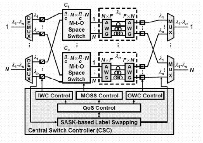
QOPS is a synchronous system which supports fixed-size packets. It is composed of two parts: the optical switch and the Central Switch Controller (CSC) (see Fig.2-1). The payload of each packet travels within the switch all-optically while its header is processed by the CSC electrically. The header which carries the label and QoS information is modulated with its payload based on the Superimposed Amplitude Shift Keying technique [8]. The packet information is used to determine its internal wavelength and related delay by the QoS Control module.

The optical switch part consists of four layers including input, output, Many-to-One Space Switch (MOSS) and output buffer. In the input part, there are N input fibers, each contains n wavelength. First we DEMUX each input fiber, and divided them into c groups according to their wavelength. Each group is connected to an optical space switch before the input wavelength is converted to its internal wavelength through a Tunable Optical Wavelength

(12)

Converter (TOWC). This internal wavelength is assigned to avoid collision within space switch and to determine whether this packet should be buffered or not. In the MOSS part there are c space switches and each takes n/c wavelengths from each input fiber. Therefore each space switch is in the size of (N n/c) (N n/c).Here the Many-to-One switch means that multiple packets coming from different inlet can be switch to the same outlet as long as they are carried by different wavelengths. And we will discuss the space switch later.

× × ×

Fig. 2-1 Architecture of QOPS

(13)

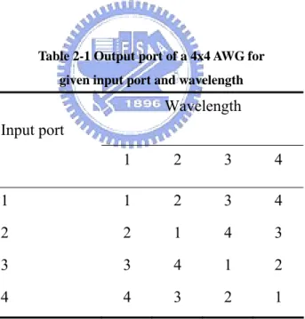
buffers. Each one is composed of a pair of Arrayed Waveguide Grating (AWG) [9] connected by F optical FDLs. Table 2-1 is an example of a AWG routing table. We can see that if two AWGs are connected by FDLs, a packet could be tuned to the same output port as the one it was sent in, no matter how it was delayed in the FDLs between those two AWGs. E.g., when a packet comes into the first AWG from input port 1 with λ

4 4×

4, it will be tuned to output

port 4 of this AWG and go to the 4-th input port of the second AWG; again it will be tuned to output port 1 of this AWG since its wavelength isλ4. Next to

the buffers, a packet is again converted to its external wavelength by a TOWC according to which output port of a buffer it comes from. After come out from buffers, packets are MUX into N output fibers.

Table 2-1 Output port of a 4x4 AWG for given input port and wavelength

Wavelength Input port 1 2 3 4 1 1 2 3 4 2 2 1 4 3 3 3 4 1 2 4 4 3 2 1

(14)

2.2 Optical Space Switch Design

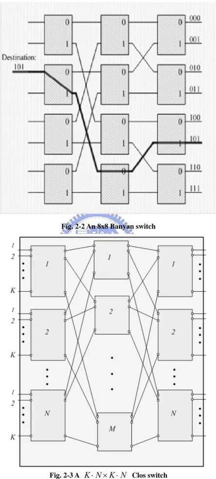
It is important to have an appropriate optical space switch for keeping internally blocking off and reducing cost of hardware manufacture. There is short-list of switches can be implemented in optical: Banyan switch and Clos switch (three-stage rearrangable and non- rearrangable). Banyan switch [2] [3] is a self-routing switch composed of several stages of switching elements (i.e., a Banyan switch has three stages, see Fig.2-2). The route through such a self-routing switch is not determined by a global controller, but each switching element (the

2 2× 8

8×

2

2× switch) in it can look at the single bit of the destination address and decide how to route the packet. However, the Banyan switch is blocking in two cases: output blocking and internally blocking. If two packets are going to the same destination, they will be routed to the same output port at the same time, and hence, collide. This is output blocking. If two packets have different input ports and destination, but have overlapping paths through switch. This is internally blocking.

Clos switch [4] [5] [6] is a three-stage non-blocking switch, and each stage is made up of a number of crossbar switches. A Clos switch is strictly non-blocking when it is always possible to connect any idle input port to any idle output port. Also, it is rearrangable non-blocking if it is possible to connect any idle input port to any idle output port, but some existing connections have to be reconfigured in order not collide. The discrepancy between these two Clos non-blocking switch is the number of switch elements in the second-stage they need. In an asynchronous switching network, the life

(15)

time of packets may overlap, thus a strictly non-blocking switch is needed that there are enough switches in second-stage for establishing any connection. In synchronous switching network, a rearrangable non-blocking switch is enough, because all packets are inputted and outputted at the same time (buffers are not considered) that they can be arranged properly just before be sent into switches.

Both Banyan switch and Clos switch would cause packets blocking when the routes of packets are not arrange properly. To avoid internally and

externally blocking, there are some schemes for them respectively [2] [4] [5]. However, those schemes for Banyan switch are more complex than those for Clos switch, especially when the scale of switch is large. Although Banyan network is easy to route a packet through its destination address, for a large size switch, the switch fabric also consist of a great number of stages which will be added into the overhead of packet’s routing path address. This results in hard to optimize the scheduling of such a large number of input requests that they will collide neither internally nor externally. On the other hand, the Clos switch is a three-stage switch no matter how the size grows. It is the number of computation that increases, not the complexity of comparing the routes which keeps blocking off. Besides, QOPS employs cluster-based wavelength sharing which is easier to implement with Clos switch.

(16)

Fig. 2-2 An 8x8 Banyan switch

N K N K⋅ × ⋅

(17)

2.3 QoS Scheduling Principles of QOPS

This all-optical switch is needed to deal with high speed and large capacity traffic, though most of the processor such as scheduling, path routing, header processing and so on couldn’t be done in optical form but electronic. Thus the scheduling and controlling will be performed in the CSC of QOPS in real-time. To do this, we should first generalize problems about the scheduling includes what conditions would result in internally blocking and externally blocking, how to utilize optical buffers and how to provide QoS. After that we could optimize the I/O request path routing and scheduling problems in next chapter.

First of all, we defined a routing path in this all-optical switch (including

the internal wavelength it carried) as where the suffixes are

illustrated as Fig.2-4. Take an example, is a path shown in

Fig.2-4 (the thick line). It is a path for a packet which inputs from the second port of the first input-cluster in the first-stage, and connected to the first output-cluster in the third-stage through the second block of the second-stage. After outputted from Clos switch, it is tuned to FDL for buffering depends on the wavelength it uses.

) , , , , , (I i s g o d P ) 4 , 2 , 1 , 2 , 1 , 2 P(

(18)

Fig. 2-4 Routing path definition

I: the I-th input port of each input blocks in the first-stage of Clos switch,

I∈{1,2,…,N }

i: the i-th input block in the first-stage of Clos switch, i∈{1,2,…,n_c}

s: the s-th block in the second-stage of Clos switch, s∈{1,2,…,M }

g: the g-th block in the third-stage of Clos switch, g∈{1,2,…,n_c_}

o: the o-th output port of each block in the third-stage of Clos switch,

o∈{1,2,…,N }

d: the wavelength it uses, d∈{1,2,…,F } (Notice that we can’t see ‘d’ from

Fig.2-3)

A question here is what size should the switch in Clos’ second-stage be? This had been answered by C.Clos [4] that for a rearrangable switch system, the number of second-stage equals to the number of output port in each switch of the first switch is enough. Thus M is set to the value v of N.

(19)

Generally speaking, there are two kinds of blocking in our switch: internally blocking and externally blocking. The former occurred within the space switches and buffers when two or more packets take the same path and wavelength. The later occurred between buffers and output fiber when packets are coming out from different FDLs in a buffer but to the same output port. Suppose there are two packets in path P(I,i,s,g,o,d) and

P(I',i',s',g',o',d'), we conclude three internally blocking and one externally

blocking situations as Fig.2-5 that if these two packets fit any of them, they collide.

Fig. 2-5 (a), (b) and (c) are those three internally blocking condition which happened when two packets take the same connection between two stages of switch with the same wavelength. For example, suppose a packet takes the path P(1,1,2,1,3,3) and another packet takes P(4,1,2,2,1,3), then they will collide between the first-stage 1 and the second-stage 2 in Clos space switch because they are going to the same channel in both wavelength 3, which would results in interference of optical signals. As for Fig.2-5 (d), the externally blocking condition, is more complex than the internal one. When a packet is coming out from certain FDL to one output port in a buffer with the wavelength which the other packet that is coming out from different FDL to the same output port in the same buffer carries, they will collide. This is so called “externally blocking”. E.g., A packet in path

P(1,1,2,1,1,2) at time 1 which will be sent to optical buffer for delaying one

time unit; another packet takes P(3,2,4,1,1,1) at one time unit later without being buffered. Therefore, both these two packets will come to output fiber

(20)

1 and be converted to the same external wavelength simultaneously, i.e. externally blocking happened. To confirm that packets won’t externally block, it is necessary to keep track of the states of packet in buffers. So we will introduce a parameter x

(

g,o,d

)

in next chapter.

Fig. 2-5 Blocking condition

(a). If i=i', s=s', d=d' and t=0, they collide between 1st-stage and 2nd-stage. (b). If s=s', g=g', d=d' and t=0, they collide between 2nd -stage and 3rd-stage. (c). If g=g', o=o', d=d' and t=0, they collide between 3rd-stage and buffers. (d). Externally blocking if two packets come to the same output port from

(21)

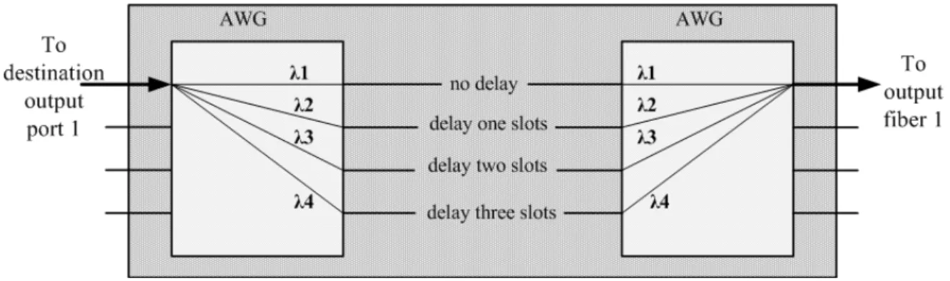
Fig. 2-6 One of Many FDL-based optical buffers

As we introduce before, the buffer is implement with two AWGs cascaded by different length of FDLs, then a packet can be buffered for different time units depends on its destination and the wavelength it uses. See Fig. 2-6, an input packet comes into this buffer through the first input port of the preceding AWG, and then be tuned to different output port that leads to varied FDLs according to its wavelength. In any case, this packet will be tuned to the output port it was sent in (output port 1 for our case in Fig.2-6) of the later AWG. A routing table for Fig. 2-6 can refer to Table 2-1. To alleviate the delay of a packet in buffers, it should be arranged appropriately that be sent to as shorter buffer-length as possible. This may need rearranging all routing paths of arriving packets in optical space switch, so that a routing path to a less buffer-length can be leave for a packet. However, all packets are in equal status (suppose that priority is not concerned), and this problem is so complex that we might achieve only an approximative optimized solution.

So far as QoS is concerned, in the former paper [1] provided primitive ability of preemption that a high-priority packet can preempt a low-priority packet which has already in system. Though we are not satisfied with this; when packets come in varied priority, it expected that a packet with

(22)

high-priority could obtain the routing path but not the one with low-priority when they either collide internally or externally. This has the scheduling gets complicated.

(23)

3 Scheduling Based on Hopfield Network

Neural network has been extensively studied for solving optimization problems since Hopfield and Tank introduced them [7]. Their neural network of the Hopfield Model (HM) has been implemented into an electric circuit that produces approximate solutions to the Traveling Salesman Problem (TSP) [10] [11] quite efficiently. It has also been apply to different switching network researches [2] [12] [13] [15] [16] [17] because of its massive parallelism which can be take as a special form of parallel computer and its highly interconnected architecture similar to those of switching networks. The HNNs will usually, but not always, converge on a maximum size match the energy function. That is, it will find a suboptimal solution, a local minimum of the energy function (we will discuss the energy function later).

3.1. Hopfield Neural Network Overview

The HNN is a single-layer feedback network with symmetric weights. There are two versions of HNN: discrete and continuous, we will discuss only the discrete one in this chapter.

A neural network has a great number of neurons where all neurons are connected to each other and each connection links has an associative weight. The functionality of the network is not derived from the operation on the

(24)

individual neurons, but from the connections between neurons. When this network performs a sequential updating process, the initial outputs are according to given initial inputs. Then the initialized outputs become the new inputs through those feedback connections, and these updated inputs again induce the new outputs. This transition process continues until the network reaches a stable state when there is no more output state changes from its input state.

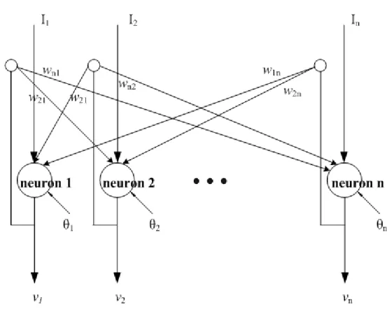
Fig. 3-1 Discrete HNN model

When the HNN is operated in discrete-time fashion, it is called a discrete Hopfield network and its structure is shown as Fig.3.1. In this figure we can see that there is an output Vj, a threshold θj, an external input Ij and plenty of

(25)

inputs for each neuron. Those inputs for the jth neuron are outputs of all other neurons through a multiplicative weight Wij for i=1, 2,… , n, i≠j, assume

there are n neurons in a network. Moreover, it is important to point out that there is no self feedback and the connected weights should be symmetric for a HNN, that is Wij=0 and Wij = Wji. The update rule for each node is

n i I V W V _i _i n i j j k i ij k i sgn , 1,2,..., 1 ) ( ) 1 ( ₌ ⎟⎟ ⎟ ⎟ ⎠ ⎞ ⎜⎜ ⎜ ⎜ ⎝ ⎛ + − =

∑

≠ = + _θ (3.1)

where sgn() is the signum function defined as

⎩ ⎨ ⎧ ≥ < − = 0 1 0 1 ) sgn( x x x (3.2)

and the superscript k represents the k-iteration of update. There are also other updating rules which the signum function sgn

( )

x is replace by different functions and are called sigmoid neuron model, McCulloch-Pitts neuron model, etc [14] . In discrete neural network, a neuron takes on only two values either 1 or -1 (also 1 or 0), and the value is determined by whether or not the total sum of a neuron’s input exceeds its threshold. This update rule should be performed in an asynchronous form which neurons are updated one by one, that is, a neuron is randomly chosen to update its output. The next neuron is also be chosen randomly to update its output with those already be updated and not yet be updated. This update rule is referred to as an asynchronous stochastic recursion of the discrete HNN.

For the purpose of evaluating the stability of the discrete HNN, we use an energy function E shown as below to character the behavior of this network.

(26)

∑

∑∑

= = = ≠ = − + − = n i i i n i i i n i n i j j j i ijVV V IV W E 1 1 1 1 2 1 _θ _(3.3)

To prove that the network will converge to a stable state, first we show that the energy function E always decreases whenever the state of any neuron changes, and then we show that it must has an absolute minimum value. When updating, assume that only one neuron Vi(k) changes its state to Vi(k+1) at a given

time. We can derive the change in energy ∆E is

(

) ( )

(

( 1) ( ) 1 1 ) ( ) 1 ( k i k i i n i n i j j j i ij k i k i V V V V W V E V E E − ⎟ ⎟ ⎟ ⎠ ⎞ ⎜ ⎜ ⎜ ⎝ ⎛ + − = − = Δ + = ≠ = +

∑∑

θ

)

i i (3.4) or

( )

net V E=− Δ Δ (3.5) where ( 1) (k). When V i k i i V V V = − Δ +

i changes from -1 to 1 (ΔVi =2), neti must be positive (from Eq.3.1) and thus ∆E will be negative; when yi changes from 1 to

-1 (ΔV_i =−2), neti must be negative and again ∆E will be negative; when Vi

does not change then and therefore ∆E will be zero. Above indicates that 0 = ΔV_i 0 ≤ ΔE (3.6)

Because yi has only two states (i.e., 1 or -1), we can conclude from Eq. (3.3)

that

∑

∑∑

= = = ≠ = − − − ≥ n i i n i i n i n i j j ij I W E 1 1 1 1 2 1 _θ _(3.7)

(27)

minimum value and it decreases whatever the states of Vi changes. Thus, for

any initial state of a HNN, it will converge to a stable state in a finite numbers of update iterations.

In fact, the above proving obeys the Lyapunov stability theorem [11].

3.2. Scheduling Problem Associated with HNN

In a HNN, the most important thing is to define the weight between each connection, which represents the information be used to solve the given problem (i.e. an optimization problem). In this section we apply the Hopfield model to our switch, so as to solve the problem such as internal wavelength and route assignment in space switches. And the information will appear in the form of constraint and cost energy functions which we illustrate in the rest of this section.

3.2.1. Non-blocking Constraints

First we transfer those blocking constraints into energy functions which conform to the format of HNN’s general energy functions. Each non-blocking constraint has a corresponding energy function, and therefore four energy functions are defined as E1、E2、E 、and 3 E4 :

(28)

(I,g,o) (I',g',o') c n i M s c n g N o F d N I c n g' N o' N I' o',d I',i,s,g', d I,i,s,g,o, V V : E ≠ = = = = = = = = = = ×

∑∑∑∑∑∑∑∑∑

0 (3.8-1) 1 1 1 1 1 1 1 1 1 1 (I,i,o) (I',i',o') c n i M s c n g N o F d N I c n i' N o' N

I' I,i,s,g,o,d I',i',s,g,o',d

V V : E ≠ = = = = = = = = = = ×

∑∑∑∑∑∑∑∑∑

0 (3.8-2) 2 1 1 1 1 1 1 1 1 1 (I,i,s) (I',i',s') c n 1 i M 1 s c n 1 g N 1 o F 1 d N 1 I c n 1 i' M 1 s' N 1

I' I,i,s,g,o,d I',i',s',g,o,d

0 V V : 3 E ≠ = = = = = = = = = = ×

∑∑∑∑∑∑∑∑∑

(3.8-3) ) (I',i',s'' (I,i,s) 0 x V : 4 E c n 1 i M 1 s N 1 I I,i,s,g,o,d g,o,d c n 1 g N 1 o F 1 d ≠ = ⎟ ⎟ ⎠ ⎞ ⎜ ⎜ ⎝ ⎛ ×

∑∑∑

= = = = = = 4) -(3.8

Where VI,i,s,g,o,d is a neuron which is set to be the value either “one” or “zero”

(“On” or “Off”) depends on whether the corresponding path P(I,i,s,g,o,d) is set up or not. And xg,o,d in E4 is a matrix represents those paths within (g,o,d) will

lead to externally blocking, this matrix is updated according to the states of buffers which should include the information of “which output port does a packet go and how many time units does it remain in buffers”. The updating can be done through looking up from a Table 3.1. For example, if a packet is in the first AWG buffers whose destination is output port 1 and it has three time units remained in buffers. From Table3.1, we know that

(29)

P(I,i,s,g=1,o=1,d=3) one slot later, it will externally block with that one

already in buffers since they will both come to the same destination, output port 1 at the same time.

Table 3-1x

(

g,o,d

)

Time remained in buffer

3 2 1

Destined Output port “o”

d=1 d=2 d=3 d=4 d=1 d=2 d=3 d=4 d=1 d=2 d=3 d=4 o=1 0 0 1 0 0 1 0 0 1 0 0 0 o=2 0 0 0 1 1 0 0 0 0 1 0 0 o=3 1 0 0 0 0 0 0 1 0 0 1 0 o=4 0 1 0 0 0 0 1 0 0 0 0 1 3.2.2. Request constraints

When an input with certain output request does not exist, there is no way such a path be setup. A constraint exists in order to keep this case off and is shown as following:

(3.9)

0 n

V

:

5 E

c n 1 i N 4 I N 1 o 2 M 1 s c n 1 g I,i,o F 1 d d I,i,s,g,o,

⎟

=

⎠

⎞

⎜

⎝

⎛

−

∑∑∑ ∑∑∑

= = = = = =

where nI,i,o means the I/O request, which nI,i,o=1 if a call request from input (I,i)

(30)

function be positive. Besides, this energy function can also be treat as a cost function since it can be interpret as “the total paths have been set up should be exactly the same with request”.

Sometimes the importance of some packets may be different from others, and we might give higher priorities to those more important packets. To do this, we modify the energy function Eq. (3.9) as:

(3.10)

0 n

V

pri

:

5 E

c n 1 i N 4 I N 1 o 2 M 1 s c n 1 g I,i,o F 1 d d I,i,s,g,o, I,i

=

⎥

⎦

⎤

⎢

⎣

⎡

⎟

⎠

⎞

⎜

⎝

⎛

−

∑∑

∑ ∑∑∑

= = = = = =

The parameter “ pri_I,_i” is added into the original E to indicate that packets 5

come from different input port

( )

I, could carry their own priorities, where i

if priority of packet come from is higher than

that of . Lp pri Hp priI,i = > I,'i' =

(

I,i

)

(

I ,'i' 3.2.3. Cost function

A cost function is used to govern the Hopfield network to converge toward some result we would like to see, but not a strictly constraint that the result must yield to. There are two cost functions in our network system: One is about the rate of acceptations which is also a constraint we introduced previously ( 5E ); the other one is about the utility of buffers, we describe it

(31)

( )

(

)

(3.11)

∑∑∑∑∑∑

= = = = = = c n 1 i M 1 s c n 1 g N 1 o F 1 d N 1 I d I,i,s,g,o,*a o,d V : 6 E

where is a matrix that defines different weights for packets, for a 4-output ports and 4-buffer-lengths, it is shown as:

(

o d a ,

)

(

)

(

)

(

)

(

)

(3.12) V a 4 V a 3 V a 2 V a V a 4 V a 3 V a 2 V a V a 4 V a 3 V a 2 V a V a 4 V a 3 V a 2 V a : 6 E c n 1 i M 1 s c n 1 g 4 1 I 1 , 4 I,i,s,g, 2 , 4 I,i,s,g, 3 , 4 I,i,s,g, 4 , 4 I,i,s,g, 2 , 3 I,i,s,g, 1 , 3 I,i,s,g, 4 , 3 I,i,s,g, 3 , 3 I,i,s,g, 3 , 2 I,i,s,g, 4 , 2 I,i,s,g, 1 , 2 I,i,s,g, 2 , 2 I,i,s,g, 4 , 1 I,i,s,g, 3 , 1 I,i,s,g, 2 , 1 I,i,s,g, 1 , 1 I,i,s,g,

∑∑∑∑

= = = = ⎪ ⎪ ⎭ ⎪ ⎪ ⎬ ⎫ ⎪ ⎪ ⎩ ⎪ ⎪ ⎨ ⎧ × + × + × + × + × + × + × + × + × + × + × + × + × + × + × + × (3.13) constant positive real is a' ' , ⎥ ⎥ ⎥ ⎥ ⎦ ⎤ ⎢ ⎢ ⎢ ⎢ ⎣ ⎡ = a 1 a 2 a 3 a 4 a 2 a 1 a 4 a 3 a 3 a 4 a 1 a 2 a 4 a 3 a 2 a 1 a(o,d)

The more delays a path is, the more cost it takes, so we give different weight coefficients: a, 2a, 3a and 4a for delay 0, delay 1, delay3 and delay 4 respectively.

These two cost functions may inhibit each other, because they are

exclusionary in terms of the total energy in HNN. For instance, when we demand the inputs not to be buffered that would result in energy function E 6 decreasing. However, some packets might therefore be blocked and the energy function E related acceptation thus decreases. 5

(32)

3.2.4. Total energy function

Total energy is therefore the sum of each constraint and cost function with a corresponding coefficient: ( ) ( ) ( ) ( ) ( ) ( )

( )

(

)

∑∑∑∑∑∑

∑∑

∑ ∑∑∑

∑∑∑

∑∑∑∑∑∑∑∑∑

= = = = = = = = = = = = = = = = = = ≠ = = = = = = = = = ≠ = = = = = = = = = ≠ = = = = = = = = = × + ⎥ ⎥ ⎦ ⎤ ⎢ ⎢ ⎣ ⎡ ⎟ ⎟ ⎠ ⎞ ⎜ ⎜ ⎝ ⎛ − × + ⎟ ⎟ ⎠ ⎞ ⎜ ⎜ ⎝ ⎛ × × + × × + × × + × × = × + × + × + × + × + × = c n i M s c n g N o F d N I d I,i,s,g,o, c n i N I N o M s c n g I,i,o F d d I,i,s,g,o, I,i c n i M s N I g,o,d d I,i,s,g,o, c n g N o F d c n i M s c n g N o F d N I c n i' M s' N I' ,o,d I',i',s',g d I,i,s,g,o, c n i M s c n g N o F d N I c n i' N o' N I' o',d I',i',s,g, d I,i,s,g,o, c n i M s c n g N o F d N I c n g' N o' N I' o',d I',i,s,g', d I,i,s,g,o, d o *a V n V pri x V V V V V V V P 1 1 1 1 1 1 1 4 1 2 1 1 1 1 1 1 1 1 1 d' , ,o' g' d g,o, 1 1 1 1 1 1 1 1 1 ,o' ,i' I' I,i,o 1 1 1 1 1 1 1 1 1 ,o' ,g' I' I,g,o 1 1 1 1 1 1 1 1 1 , 2 U 2 S 2 X 2 R 2 Q 2 E6 U E5 S E4 X E3 R E2 Q E1 P E Compare to the general formulation expanded from Eq. (3.3):

(33)

(3.15) ) , , , , I, ( I,,, , , I,,, ,, ) , , , , I, ( ) , , , , I, ( )' ,' ,' ,' ,' , I' ( )' ,' ,' ,' ,' , I' ( (I,,, ,, ),(I', ,' ,' ,' ,' )' I,,, , , I',,' ,' ,' ,' '

∑

+ − = Ε ≠ d o g s i isgod isgod d o g s i d o g s i d o g s i d o g s i isgod i s g o d isgod i s g o d V I V V w 2 1

we can get and by comparing their coefficients.

The details are shown as below

)' ,' ,' ,' ,' , I' ( ), , , , , I, ( isgod i s g o d W I_I,_i_,_s_,_g_,_o_,_d

(

)

{

}

(

)

{

}

(

)

{

}

(3.16) pri 1 1 1 i I, ' , ' , I' I, ' s , ' , I' I, ' , ' , ' , ' , ' , I' I, ' , ' , ' s , ' , ' , I' I, ' , ' , ' , ) d' , o' , g' , s' , i' , (I' d), o, g, s, i, (I, × × × × − × × − × × × × − × × − × × × × − × × − × × × × − = o o i i s i i d d o o g g o o i i d d g g s o o g g d d s s i i S R Q P W δ δ δ δ δ δ δ δ δ δ δ δ δ δ δ δ δ δ δ δ δ and (3.17) pri ) , ( U , , , , i I, ) , , , , , (Iisgod Iio xgod 2 X n S d o a 2 I = × − × × + ×

and δ is the impulse function

(3.18) y x if 0 y x if 1 y x, ⎩ ⎨ ⎧ ≠ = =

δ

(34)

4 Experimental Results

In last chapter we proposed a HNN model to schedule input packets for QOPS. In this chapter we compare its performance with other scheduling algorithms Random Assignment (RA) and Sequential Assignment (SA) through experimenting on computers. RA schedules inputs packets by randomly assigning routing paths and wavelengths; and SA assigns packets one after another. Besides, when a path is assigned to one packet, paths which would collide with it are ruled out and the next packet is assigned a path from the rest unless there is no path can be assigned. The advantages for RA are simple and fast, but packets lost because of collision. On the other hand, SA is more complex and time-consuming but low lost probability. Before showing above comparisons, we set details of our experiment and discuss features of coefficients of HNN energy function.

For the purposes of evaluating the performance of the proposed scheduling formula of QOPS based on HNN model we fix the numbers of input and output fibers N, wavelength channels in each fiber (n), space switches (c) and internal wavelength (F), where we assume N=4, n=6, c=2 and

F=4 in our simulation as Fig.4-1. Although each input fiber takes six

wavelengths, we can regard n=6 as a portion of total wavelengths in each fibers which are aggregated into one of those space switches. There could be still many wavelengths are aggregated into other space switches. However, we can extend simulation result of one portion to remnants since they should have the same behaviors besides the wavelengths they take in input fibers and

(35)

output fibers. For the same reason, we can experiment only on the half part of QOPS that is, n=3 and c=1.

In last chapter we design a HNN model to solve the paths scheduling optimization problem in QOPS. But the feature of preemption for high priority packet mentioned in chapter 1 is not covered in the HNN model we design. Moreover, the non-externally blocking constrain energy function will keep packets not to be routed to any output port in some specific wavelength which will lead to externally blocking, and therefore it is not necessary for packets to preempt any packet has already in delay line. For this reason the experiment does not include the preemption when the non-externally blocking energy function is considered, and vice versa.

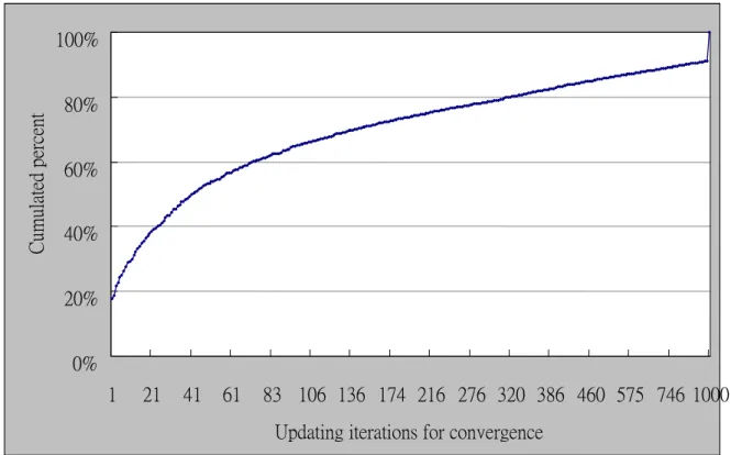
The experiment was executed in Language C. The number of iterations is limited under 80 times, that is, we will stop the updating of neurons no matter the HNN has converged or not. If it has converged, we can transfer the status of neurons to routing paths. What if it hasn’t converged? A set of solution for routing paths is still needed anyway. Thus, some compensation is applied on it to function as a filter that filters out those illegal routing paths transferred from status of neurons. The distribution of iterations for convergence is shown in Fig.4-2. About 60% would converge beneath 80 iterations; about 90% would converge beneath 800 iterations; and about 9% would converge after more than 1000 iterations.

The number of input batches for test is not fastened, but varies with the variation of throughputs for each test input batch. In other word, the execution

(36)

stops when the throughput varies no more than 0.5% of its mean value for this test for present. Following we will show the results of experiment in two cases: non-preemption and preemption. Both them include HNN model with and without QoS issue.

(37)

0% 20% 40% 60% 80% 100% 1 21 41 61 83 106 136 174 216 276 320 386 460 575 746 1000 Updating iterations for convergence

Cumulat

ed percent

Fig. 4-2 Distribution of iterations for convergence

(38)

The coefficients which affect the performance (throughput) most are that of acceptation constraint and buffer utility cost function. In Fig.4-3, both throughputs of HNN methods with and without preemption decrease to be zero when the value of coefficient U increases to twice of coefficient S. Here coefficients of other constraints are fixed as following: P=Q=R=50,

1

, = Hp = Lp =

pri_I_i (Hp for a high priority packet and for a low priority

packet), X=50 for non-preemption, X=0 for preemption. Apparently, HNN without preemption, which non-externally blocking constraint is considered, provides better performance than HNN with preemption.

Lp

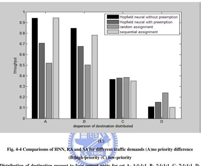
SA scheduling algorithm can provide results approximates those of exhaust algorithm because it assigns paths to packets as possible as it can until there is no illegal paths could be assigned. Fig.4-4(A) shows that for different traffic demands A, B, C, and D, HNN without preemption performs as good as SA does. In this figure, the throughput decreases as the distribution of destination request to four output ports gets wider because of the increasing of externally blocking probability.

Now we enable the QoS functionality in our Hopfield neural system model which is achieved by adjust the coefficient in Eq.(3.10) where

for a high priority packet and for a low priority packet.

Fig.4-4(B) and Fig.4-4 (C) are throughputs of high- and low-priority for HNN, RA ad SA. We can see that HNN without preemption method can provides priority differentiation in the pattern similar to SA.

i I

pri_,

Hp

(39)

(40)

(B)

(C)

Fig. 4-4 Comparisons of HNN, RA and SA for different traffic demands (A)no priority difference (B)high-priority (C) low-priority

Distribution of destination request to four output ports for set A- 1:1:1:1, B- 2:1:1:1, C- 7:1:1:1, D- 91:3:3:3

(41)

5 Conclusions and Discussions

In this paper we apply HNN to a switching system called QOPS for metro WDM networks to solve the complex problem of routes assigning. The Hopfield model for this switch we designed also provides QoS differentiation by means of giving diverse weights in energy functions of HNN model to obtain different throughput and buffering. In chapter 4, we simulate the performance through not only Hopfield neural method but also optical packet preemption. Both of them could satisfy low loss probability or low-delayed traffic demands by adjusting coefficients and weights in energy functions. The result shows that the system can provide QoS according to optical packet’s priority.

QOPS has been designed and experimented in our related research. The study in this paper aims at designing an algorithm that scheduling the path routes and internal wavelength assignment for QoS Control module of QOPS. In future works, the HNN model will be apply to the FPGA-based QoS Control module and Central Switch Controller.

(42)

Reference

1. Yuang, M.C.; Tien, P.L.; Shih, J.; Lee, S.S.W.; Yu-Min Lin; Chen, J.J.; “A QoS optical packet-switching system for metro WDM networks”, Optical Communication ECOC 2005. 31st European Conference, vol. 3, pp.351 - 352, 25-29 Sept. 2005

2. T.X. Brown, KH Liu, “Neural Network Design of a Banyan Network Controller”, Selected Areas in Communications, IEEE Journal, vol 8, Issue 8,pp.1428-1438, Oct 1990

3. L.G. Alberto, I. Widjaja, “Communication network”, McGraw-Hill,2004

4. C. Clos, “A study of non-blocking switching networks,” Bell Syst. Tech. J.,

vol. 32, pp. 406–424, 1953.

5. Cheyns, J, et. al.,” Clos lives on in optical packet switching”, Communications Magazine, IEEE vol. 42, Issue 2, pp.:114 – 121, Feb 2004

6. Liotopoulos, F.K., “A terabit electro-optical Clos switch architecture” High Performance Switching and Routing, IEEE Workshop, pp.265 – 270, 29-31 May 2001.

7. J. J. Hopfield and D. Tank, “Neural computation of decisions in optimization problems,” Biol. Cybern., vol. 52, pp. 141–152, 1985.

8. Y. Lin, M. Yuang, S. Lee, and W. Way, ”Using Superimposed ASK Label in a 10Gbps Multi-Hop All-Optical Label Swapping System”, J. Lightwave Technol., vol. 22, pp.351-361 2004

9. H. Takahashi, et al., "Transmission characteristics of Arrayed Waveguide NxN Wavelength Multiplexer",IEEE J. Lightwave Tech., vol.13, no.2,

(43)

1995.

10. E. L. Lawler, J. K. Lenstra, R. Kan, and P. B. Shmoys, “The

TravelingSalesman Problem”, New York: Wiley, 1985.

11. C. T. Lin and C. S. G. Lee, “Neural Fuzzy Systems: A Neuro-Fuzzy Synergism to Intelligent Systems “, Prentice Hall, 1996.

12. T.X. Brown, “Neural networks for switching”, IEEE Communications Mag.,pp.72-81,Nov,1989

13. N. Funabiki, Y. Takefuji, and K.C. Lee, “A neural network model for traffic controls in multistage interconnection networks”, IJCNN 1991, vol.II, pp.II A-898.

14. ──, “Comparisons of Seven Neural Network Models on Traffic Control Problems in Multistage Interconnection Networks”, IEEE Transactions on Computers, vol. 42, no.4, pp.497-501, April 1993.

15. N. Funabiki and Y. Takefuji, “A parallel algorithm for traffic control problems in three-stage connecting networks”, Journal of Parallel and Distributed Computing, in press.

16. Park, Y.-K., Cherkassky, V. “Neural network controller for rearrangeable switching networks”, Neural Networks, 1993., IEEE International Conference, vol.3, pp.1896-1901, 03/28-04/01/ 1993

17. Yong Li, et al., “A positively self-feedbacked HNN architecture for crossbar switching”, Circuits and Systems I: Regular Papers, IEEE Transactions on [see also Circuits and Systems I: Fundamental Theory and Applications, IEEE Transactions on] vol. 52, Issue 1, pp.200 -206, Jan. 2005

光纖封包交換系統交換機的高服務品質排程

國 立 交 通 大 學

電信工程學系

碩 士 論 文