A note on a 2-approximation algorithm for the
MRCT problem
Bang Ye Wu Kun–Mao Chao
March 12, 2004
1
Introduction
Consider the following problem in network design: given an undirected graph with nonnegative delays on the edges, the goal is to find a spanning tree such that the average delay of communicating between any pair using the tree is minimized. The delay between a pair of vertices is the sum of the delays of the edges in the path between them in the tree. Minimizing the average delay is equivalent to minimizing the total delay between all pairs of vertices using the tree.
In general, when the cost on an edge represents a price for routing mes-sages between its endpoints (such as the delay), the routing cost for a pair of vertices in a given spanning tree is defined as the sum of the costs of the edges in the unique tree path between them. The routing cost of the tree itself is the sum over all pairs of vertices of the routing cost for the pair in this tree, i.e., C(T ) =Pu,vdT(u, v), where dT(u, v) is the distance between
u and v on T . For an undirected graph, the minimum routing cost span-ning tree (MRCT) is the one with minimum routing cost among all possible
spanning trees.
Unless specified explicitly in this note, a graph G is assumed to be simple and undirected, and the edge weights are nonnegative. Finding an MRCT in a general edge-weighted undirected graph is known to be NP-hard. In this note, we shall focus on the 2-approximation algorithms. Before going into the details, we introduce a term, routing load, which provides us an alternative formula to compute the routing cost of a tree.
Definition 1: Let T be a tree and e ∈ E(T ). Assume X and Y are the two subgraphs that result by removing e from T . The routing load on edge
For any edge e ∈ E(T ), let x and y (x ≤ y) be the numbers of vertices in the two subtrees that result by removing e. The routing load on e is 2xy = 2x(|V (T )| − x). Note that x ≤ n/2, and the routing load increases as
x increases. The following property can be easily shown by the definition.
Fact 1: For any edge e ∈ E(T ), if the numbers of vertices in both sides of e are at least δ|V (T )|, the routing load on e is at least 2δ(1 − δ)|V (T )|2.
Furthermore, for any edge of a tree T , the routing load is upper bounded by |V (T )|2 2.
For a graph G and u, v ∈ V (G), we use SPG(u, v) to denote a shortest
path between u and v in G. In the case where G is a tree, SPG(u, v) denotes
the unique simple path between the two vertices. By defining the routing load, we have the following formula.
Lemma 1: For a tree T with edge length w, C(T ) =Pe∈E(T )l(T, e)w(e).
In addition, C(T ) can be computed in O(n) time.
Proof: Let SPT(u, v) denote the simple path between vertices u and v
on a tree T . C(T ) = X u,v∈V (T ) dT(u, v) = X u,v∈V (T ) X e∈SPT(u,v) w(e) = X e∈E(T ) X u∈V (T ) |{v|e ∈ SPT(u, v)}| w(e) = X e∈E(T ) l(T, e)w(e).
To compute C(T ), it is sufficient to find the routing load on each edge. This can be done in O(n) time by rooting T at any node and traversing T in a postorder sequence.
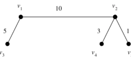
Example 1: Consider the tree T in Figure 1. The distances between ver-tices are as follows:
dT(v1, v2) = 10 dT(v1, v3) = 5 dT(v1, v4) = 13
dT(v1, v5) = 11 dT(v2, v3) = 15 dT(v2, v4) = 3
dT(v2, v5) = 1 dT(v3, v4) = 18 dT(v3, v5) = 16
v 1 v2 v 3 10 v 4 v5 5 3 1
Figure 1: An example illustrating the routing loads.
The routing cost of T is two times the sum of the above distances since, for
vi and vj, both dT(vi, vj) and dT(vj, vi) are counted in the cost. We have
C(T ) = 192.
On the other hand, the routing load of edge (v1, v2) is calculated by
l(T, (v1, v2)) = 2 × 2 × 3 = 12
since there are two and three vertices in the two sides of the edge, respec-tively. Similarly, the routing loads of the other edges are as follows:
l(T, (v1, v3)) = 8 l(T, (v2, v4)) = 8 l(T, (v2, v5)) = 8.
Therefore, by Lemma 1, we have
C(T ) = 12 × 10 + 8 × 5 + 8 × 3 + 8 × 1 = 192.
At the first sight of the definition C(T ) =Pu,vdT(u, v), one may think
that the weights of the tree edges are the most important to the routing cost of a tree. On the other hand, by Lemma 1, one can see that the routing loads also play important roles. The routing loads are determined by the topology of the tree. Therefore the topology is crucial for constructing a tree of small routing cost. The next example illustrates the impact of the topology by considering two extreme cases.
Example 2: Let T1 be a star (a tree with only one internal node) in which
each edge has weight 5, and T2 be a path in which each edge has weight 1
(Figure 2). Suppose that both the two trees are spanning trees of a graph with n vertices. In the aspect of total edge weight, we can see that T2 is
better than T1. Let’s compute their routing costs. For T1, the routing load
of each edge is 2(n − 1) since each edge is incident with a leaf. Therefore, by Lemma 1, C(T1) = 10(n − 1)2.
v 1 v2 v3 vn T 2 1 1 1 ... T 1 v 2 v 1 v 3 5 5 5 ... 5 5 5 v n
Figure 2: Two extreme trees illustrating the impact of the topology.
Let T2 = (v1, v2, . . . , vn). Removing an edge (vi, vi+1) will result in two
components of i and n − i vertices. Therefore the routing loads are 2(n − 1), 2 × 2 × (n − 2), . . . , 2 × i × (n − i), . . . , 2(n − 1). By Lemma 1, C(T2) = X 1≤i≤n−1 2i(n − i) = n2(n − 1) − n(n − 1)(2n − 1) 3 = n(n − 1)(n + 1) 3 .
So T2 is much more costly than T1 when n is large.
In the following sections, we shall discuss the complexity and several approximation algorithms for the MRCT problem. In this note, by mrct(G), we denote a minimum routing cost spanning tree of a graph G. When there is no ambiguity, we assume that G = (V, E, w) is the given underlying graph, which is simple, connected, and undirected. We shall also useT and mrct(G)b
interchangeably.
2
Approximating by a Shortest-Paths Tree
2.1 A simple analysis
Since all edges have nonnegative length, the distance between two vertices is not decreased by removing edges from a graph. Obviously dT(u, v) ≥
dG(u, v) for any spanning tree T of G. We can obtain a trivial lower bound of the routing cost.
Let r be the median of graph G = (V, E, w), i.e., the vertex with minimum total distance to all vertices. In other words, r minimizing the function
f (v) =Pu∈V dG(v, u). We can show that a shortest-paths tree rooted at r
is a 2-approximation of an MRCT.
Theorem 2: A shortest-paths tree rooted at the median of a graph is a 2-approximation of an MRCT of the graph.
Proof: Let r be the median of graph G = (V, E, w) and Y be any shortest-paths tree rooted at r. Note that the triangle inequality holds for the distances between vertices in any graph without edges of negative weights. By the triangle inequality, we have dY(u, v) ≤ dY(u, r) + dY(v, r) for any vertices u and v. Summing up over all pairs of vertices, we obtain
C(Y ) =X u X v dY(u, v) ≤ nX u dY(u, r) + n X v dY(v, r) = 2nX v dY(v, r).
Since r is the median, PvdG(r, v) ≤
P
vdG(u, v) for any vertex u, it
follows X v dG(r, v) ≤ n1 X u,v dG(u, v).
Recall that, in a shortest-paths tree, the path from the root to any vertex is a shortest path on the original graph. We have dY(r, v) = dG(r, v) for each
vertex v, and consequently
C(Y ) ≤ 2nX v dG(r, v) ≤ 2 X u,v dG(u, v). By Fact 2, Y is a 2-approximation of an MRCT.
The median of a graph can be found easily once the distances of all pairs of vertices are known. By Theorem 2, we can have a 2-approximation algorithm and the time complexity is dominated by that of finding all-pairs shortest path lengths of the input graph.
Corollary 3: An MRCT of a graph can be approximated with approxi-mation ratio 2 in O(n2log n + mn) time.
The approximation ratio in Theorem 2 is tight in the sense that there exists an extreme case for the inequality asymptotically. Consider a complete graph with unit length on each edge. Any vertex is a median of the graph and the shortest-paths tree rooted at a median is just a star. The routing cost of the star can be calculated by
2(n − 1)(n − 2) + 2(n − 1) = 2(n − 1)2.
Since the total distance on the graph is n(n − 1), the ratio is 2 − (2/n). However, the analysis of the extreme case does not imply that the ap-proximation ratio cannot be improved. It only means that we cannot get a more precise analysis by comparing with the trivial lower bound. It can be easily verified that, for the above example, the star is indeed an optimal so-lution. The problem is that we should compare the approximation solution with the optimal, but not with the trivial lower bound. Now we introduce another proof of the approximation ratio of the shortest-paths tree. The analysis technique we used is called solution decomposition, which is widely used in algorithm design, especially for approximation algorithms.
2.2 Solution decomposition
To design an approximation algorithm for an optimization problem, we first suppose that X is an optimal solution. Then we decompose X and construct another feasible solution Y. To our aim, Y is designed to be a good approx-imation of X and belongs to some restricted subset of feasible solutions, of which the best solution can be found efficiently. The algorithm is designed to find an optimal solution of the restricted problem, and the approximation ratio is ensured by that of Y. It should be noted that Y plays a role only in the analysis of approximation ratio, but not in the designed algorithm. In the following, we show how to design a 2-approximation algorithm by this method.
For any tree, we can always cut it at a node r such that each branch contains at most half of the nodes. Such a node is usually called a centroid of the tree in the literature. For example, in Figure 3(a), vertex r is a centroid of the tree. The tree has nine vertices. Removing r from the tree will result in three subtrees, and each subtree has no more than four vertices. It can be easily verified that r is the unique centroid of the tree in (a). However, for the tree in (b), both r1 and r2 are centroids of the tree.
Suppose that r is the centroid of the MRCTT . If we construct a shortest-b
paths tree Y rooted at the centroid r, the routing cost will be at most twice that of T . This can be easily shown as follows. First, if u and v are twob
r r1 r2
(a) (b)
Figure 3: A centroid of a tree.
nodes not in a same branch, dTb(u, v) = dTb(u, r) + dTb(v, r). Consider the total distance of all pairs of nodes onT . For any node v, since each branchb
contains no more than half of the nodes, the term dTb(v, r) will be counted in the total distance at least n times, n/2 times for v to others, and n/2 times for others to v. Hence, we have C(T ) ≥ nb PvdTb(v, r). Since, as in the proof of Theorem 2, C(Y ) ≤ 2nPvdG(v, r), it follows that C(Y ) ≤ 2C(T ). Web
have decomposed the optimal solution T and construct a 2-approximationb Y . Of course, there is no way to know what Y is since the optimal T isb
unknown. But we have the next result.
Lemma 4: There exists a vertex such that any shortest-paths tree rooted at the vertex is a 2-approximation of the MRCT.
By Lemma 4, we can design a 2-approximation algorithm which constructs a shortest-paths tree rooted at each vertex and chooses the best of them. Since there are only n vertices and a shortest-paths tree can be constructed in
O(n log n + m) time, the algorithm runs in polynomial time. By Lemma 1,
the routing cost of a tree can be computed in O(n) time. Consequently the algorithm has time complexity O(n2log n + mn), the same result as in Corollary 3.