The world price of exchange risk in the
Paci®c Basin equity markets
P E T E R S H Y A N - R O N G C H O U , Y I N - C H I N G J A N *{ and M A O - W E I H U N G}
Department of Finance Operations, National Kaohsiung First University of Science and Technology. 1, University Road, Yuanchau, Kaohsiung, Taiwan, ROC, { Department of Industrial Engineering and Management, National Chin-Yi Institute of Technology. 35, Lane 215, ChungShan Road, Taiping City, Taichung, Taiwan, ROC and } Department of International Business, National Taiwan University. 50, Lane 144, Keelung Road, Section 4, Taipei, Taiwan, ROC
This paper investigates whether the foreign exchange risk is priced in the Paci®c Basin equity markets. The test was performed in the conditional version which allows the world prices of market risk and exchange risk to vary over time. Being parsimonious, a principal component analysis is taken on these Paci®c Basin interest rates to extract the common exchange rate factors. The results show that the international asset pricing model with exchange risk premia is better than the international asset pricing model without exchange risk premia to describe the Paci®c Basin stock returns. This implies the world prices of exchange risk are present in the Paci®c Basin equity markets.
I . I N T R O D U C T I O N
Accurate models of internationa l asset pricing are vital to understan d and predict the behaviour of international invest-ment in an increasingl y integrated world. Although Solnik (1974a) , Stulz (1981) and Adler and Dumas (1983) had suc-cessfully extended the domestic Asset Pricing Model (APM) to internationa l APM,1the empirical tests of their models did not provide convincing evidence to support the international APM. There are several approache s that can be used to test the internationa l APM. First, the unconditiona l version of the international APM, in which the second moments are constant and the market prices of risk are unspeci®ed, can be used. Solnik (1974b) and Stehle (1977) found evidence in favour of the international Capital Asset Pricing Model (CAPM),2but in their work national factors also played an important role in determining the price behaviour of equity returns. Wheatley (1988) and Cumby (1990) provided little
evidence against the unconditional version of the inter-national consumption-base d APM described in Stulz (1981).3 Second, a more recent approach is to use the con-ditional form. This formulation lets the risk premium or market price of the risk vary over time. For example, Harvey (1991) found that the international CAPM with time-varying risk premium was useful in characterizing the dynamics of cross-section expected returns in most developed countries, but it did not perform well for other developed countries. Third, one can specify second moment behaviour and assume that the coe cient of risk aversion is constant. The evidence of Engel and Rodrigues (1989) and Thomas and Wickens (1993) showed that the international CAPM performs much better when the covariance matrix is not constant over time, but provided little explanatory power for expected relative rates of return.
Although the above studies did not reject the inter-national CAPM, the results seemed inconsistent with the
Applied Financial Economics ISSN 0960±3107 print/ISSN 1466±4305 online # 2002 Taylor & Francis Ltd
http://www.tandf.co.uk/journals DOI: 10.1080 /0960310021012502 8
361
* Corresponding author.
1See the review of Stulz (1994). 2
The international CAPM was developed by Solnik (1974a) under the assumption of independence between exchange and market risks.
3In contrast to the results for the full sample, from January 1974 to December 1987, Cumby found that observed real equity returns are
observed cross-section rates of return for some markets. This phenomenon has led to empirical research to deter-mine whether there are other risk premia which impact the behaviour of equity returns. In fact, the foreign exchange premium, which is acquired under the deviation of Purchasing Power Parity (PPP), has already been presented in the international APM of Adler and Dumas (1983).4 However, the unobservable wealth weighted risk tolerance, on which the weights on the covariances of asset returns with in¯ation depend, make the model di cult to test. The work of Dumas (1994) and Dumas and Solnik (1995) sub-stituted the interest rate for the in¯ation rate and success-fully derived world prices of foreign exchange risk from the wealth weighted risk tolerance. While their evidence sup-ported the existence of foreign exchange risk premia, there would be too many parameters to get risk premia estimates stable under the conditional approach, so only a small number of countries could be examined simultaneously. Another simpli®cation is to aggregate the exchange rate factor by weighted average, e.g., Ferson and Harvey (1993) and Harvey (1995). However, they did not provide an adequate theoretical basis for their choice of weights.
This study takes a principal component analysis on the interest rates to construct the exchange rate factors. This method avoids the shortcomings of the weighted average approach and makes the model parsimonious. In fact, the principal component analysis we used is similar in spirit to the international Arbitrage Pricing Theory (APT) postu-lated by Solnik (1983). If the ®nancial markets are integrated, any economical shocks would in¯uence endogenous variables such as exchange rates and interest rates. For instance, signi®cant de®cit ®scal policy by a government may increase the interest rate, leading to an appreciation of this country’s currency. Because there are so many shocks and so many countries, in which shocks could originate, one cannot identify these factors directly. Conversely, with the principal component analysis, these factors can be reasonably extracted.
The aim of this study is to test whether the foreign exchange risk is priced in Paci®c Basin equity markets by international APM with principal component analysis. If the risk is priced, hedging will be valuable to investors; see, e.g. Perold and Schulman (1988). To take advantag e of potential diversi®cation bene®ts from investing in Paci®c Basin markets, we need to know whether there exists for-eign exchange risk in this region.
The empirical evidence shows that the international APM with exchange risk premia performs better than the international APM without exchange risk premia, implying that the foreign exchange risk is priced in Paci®c Basin equity markets. The paper is organized as follows.
Section II outlines the methodology. Section III describes the data; section IV presents the empirical results. Some concluding remarks are presented in the ®nal section.
I I . M E T H O D O L O G Y
If there are L ‡ 1 countries and a set of N ˆ n ‡ L ‡ 1 assets which compose of n equities and L ‡ 1 nominal bank deposits, the international APM developed by Adler and Dumas (1983) can be written as:
riˆ …1 ¡ 1=¬m† X i …1 ¡ ¬l†wl¼li;º X l …1 ¡ ¬l†wl ‡ …1=¬ m †X N kˆ1 wmk¼i;k …1†
where riis the excess return on the security i, which subtracts the risk-free rate on the numeraire currency, and ¬mˆPlw
l
¬l=Plwl is the average individual’s risk toler-ance, ¬l, weighted by their own wealth, wl. While wmk is the weight on the market portfolio, ¼li;º and ¼i;k are the covar-iances of security i with the investors’ rate of in¯ation and market portfolio, respectively. Unfortunately , the ®rst term on the right-hand side is unobservable . To get an empirical asset pricing model, the ®rst term must be aggregate d under the assumption that investors from the same country use the same de¯ator and therefore have the same covariance term ¼i;ºacross countries. Then, one has the multi-beta CAPM:
riˆ …1 ¡ 1=¬m† XL jˆ1 yj¼i;º‡ …1=¬m† XN kˆ1 wmk¼i;k …2† where yjˆ P l……1 ¡ ¬ l †wl=Pl…1 ¡ ¬ l †wl† is the national wealth weighted average risk tolerance, where the ®rst sum-mation is over all the investors of the same country and the summation in the denominator is over all the world’s inves-tors. Hence, there exist L risk premia concerned for in¯a-tion rate and one risk premium for the world market portfolio. When the prices of risk are allowed to be time-varying, the conditional version of Equation 2 satis®es
E…ritj«t¡1† ˆ XL
jˆ1
¶j;t¡1cov…rit; rjtj«t¡1†
‡ ¶m;t¡1cov…rit; rmtj«t¡1† …3† where E…¢† is expectation operator, rit is the excess return on security i from time t ¡ 1 to t, rmtis the excess return on the world market portfolio, rjt is the excess return on the currency deposit of country j, and «t¡1is the information set. The coe cient ¶j;t¡1, which is equal to …1 ¡ …1=¬m††yj, represents the time-varying world prices of exchange risk, and the coe cient ¶m;t¡1, which is equal to 1=¬m,
repre-4The foreign exchange premium, which was also presented in Solnik (1974a) and Stulz (1981), was designated as in¯ation premium in
sents the time-varying world price of market risk. We replace the in¯ation premium Oi;º with cov…rit; rjtj«t¡1†, which is the conditional covariance of the excess return rit and rjt. The reasoning of this substitution lies in the low frequency and insensitivity of the in¯ation rate. Consequently, this substitution makes the international APM of Adler and Dumas (1983) similar to the n ‡ 1 funds theorem of Solnik (1974a).
To test this conditional version of the international APM, one needs to know how the investors perceive the world prices of exchange risk and market risk. It is assumed that the information set «t¡1 is generated by a vector of z predetermined instrumental variables zt¡1. As a result, these variables z can serve as proxies for the state variables. It is also assumed that there exists a linear rela-tionship between the world prices of risk and these state variables, i.e.,
¶j;t¡1ˆ zt¡1¯j ¶m;t¡1ˆ zt¡1¯m
…4†
where the ¯j and ¯m are z time-invariant vectors of par-ameter. From the above assumption, Equation 3 becomes:
E…ritjzt¡1† ˆ XL
jˆ1
zt¡1djcov…rit; rjtjzt¡1†
‡ zt¡1¯mcov…rit; rmtjzt¡1† …5† If the exchange risks are not priced, the ®rst term of the right-han d side of Equation 5 would disappear, which is the conditional form of Sharpe-Lintner asset pricing model. Following Dumas and Solnik (1995), the model that contains the prices of exchange risk is referred to as `international’ , and the model that does not contain such terms is referred to as `classic’.
Equation 5 satis®es the ®rst-order conditions from a standard representative agent’s discrete-time utility maxi-mization problem (see Lucas, 1982), i.e.,
E…Mt…1 ‡ rf ;t¡1†jzt¡1† ˆ 1 E…Mtritjzt¡1† ˆ 0 …6† where Mt…1 ¡ PL jˆ1zt¡1¯jrjt¡ zt¡1¯mrmt†=1 ‡ rf ;t¡1†, which is the pricing kernel implied by the mean-variance theory of international asset pricing (see Hansen and Jagannathan , 1991), and rf ;t¡1 is the conditionally risk-free rate on numeraire currency. Under rational expectation, Equation 6 satis®es:
et ˆ 1 ¡ Mt…1 ‡ rf ;t¡1† hit ˆ Mtrit
…7†
where et and hit are innovations. Taking a little algebra, Equation 7 becomes: etˆ XL jˆ1 zt¡1¯jrjt‡ zt¡1¯mrmt hitˆ rit¡ ritet …8†
Let "tˆ …et; ht†, Equation 6 implies E…"tjzt¡1† ˆ 0. Therefore, Hansen’s (1982) generalized method of moment (GMM) estimation can be used to estimate these multiple equations.5
If there are L ‡ 1 portfolios to be tested, there will be z …L ‡ 1† parameters which need to be estimated. The number of parameters may be too large to achieve stability in this model. For the reasons of stability and parsimony, a principal component analysis to the interest rates is taken and the L interest rates reduced to p factors. When the factor analysis is taken, the factor scores obtained by the weighted least square method are equivalent to the principal compon-ents. Hence, the spirit of the principal component analysis in this step lies in extracting the common factors that in¯uence those interest rates.
In order to test the adequateness of the conditional APM for Paci®c Basin equity markets, Hansen’s test of overiden-tifying restrictions can be used. For the L ‡ 1 equities to be tested, there will be …L ‡ 2† £ z orthogonality conditions andz £ …p ‡ 1† parameters. It follows that the J statistic of Equation 8 is asymptoticall y distributed as chi-squared …À2† with the number of degrees of freedom equal to z £ …L ‡ 1 ¡ p†, which is the number of overidentifying restrictions.
I I I . D A T A A N D S U M M A R Y S T A T I S T I C S
In this study, six equity markets were taken into account: Hong Kong, Japan, Korea, Malaysia, Thailand and the USA. These data were drawn from the Paci®c-Basin Capital Markets (PACAP) database, except for the US data which came from the German and International Financial (GERFIN) database. The market returns from the PACAP database were value weighted market returns with cash dividend reinvested, while the market return for the USA was the monthly rate of change of Standard and Poor’s 500 Composite Share Index (S&P500). The Morgan Stanley Capital International (MSCI) world index was treated as the world market portfolio. During this stage, we must assume that the MSCI world index is an e cient benchmark portfolio. If the MSCI world index is not e -cient, there may be no relationship between the world price of market risk and the expected return. Moreover, empiri-cal tests of the mean-variance e ciency of the MSCI world
5Based on Ferson and Foerster (1994), iterated GMM were used, which was proven to be superior to the two step GMM in a ®nite
index, as far as is known, have never refuted, e.g., Harvey and Zhou (1993). Available monthly data cover the period from April 1980 to December 1993. This period was chosen by most Paci®c Basin countries to open their capital mar-kets, and as a result, mitigate the eVect of market segment on the pricing model.
All the market returns were measured in numeraire cur-rency, the US dollar. The excess return on an equity market was the return on that market translated into dollars minus the dollar one-month nominally risk-free rate, which was the Fama/Bliss risk-free rate that came from the Center for Research in Security Price (CRSP). The excess return on a currency deposit was the one-month interest rate of that currency compounded by the rate of change of the exchange rate relative to the US dollar, minus the dollar one-month risk-free rate. The one-month interest rate of Japan was the
Euro money market middle rate that came from GERFIN, and the other four were money market rates which came from the Internationa l Monetary Fund (IMF).
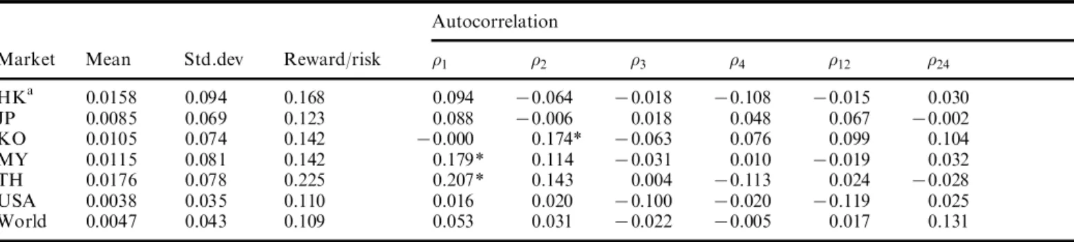
The instrumental variables were common to all markets because we were interested in characterizing the common state variables across all markets. A number of researchers have found that some economical variables can capture the dynamics of equity return. Following Harvey (1991), the following economic variables were used as an information set: the world market return, the S&P500 dividend yield (from the US Financial database, USFIN), the US yield spread between Moody’s Baa and Aaa bonds (from USFIN), the excess return on a three month bill (from USFIN), and a dummy variable for the month of January. Table 1 presents the summary statistics for the excess equity returns and instrumental variables. Panel A shows
Table 1a. Summary statistics for the market returns and instrumental variables: excess returns Autocorrelation
Market Mean Std.dev Reward/risk »1 »2 »3 »4 »12 »24
HKa 0.0158 0.094 0.168 0.094 70.064 70.018 70.108 70.015 0.030 JP 0.0085 0.069 0.123 0.088 70.006 0.018 0.048 0.067 70.002 KO 0.0105 0.074 0.142 70.000 0.174* 70.063 0.076 0.099 0.104 MY 0.0115 0.081 0.142 0.179* 0.114 70.031 0.010 70.019 0.032 TH 0.0176 0.078 0.225 0.207* 0.143 0.004 70.113 0.024 70.028 USA 0.0038 0.035 0.110 0.016 0.020 70.100 70.020 70.119 0.025 World 0.0047 0.043 0.109 0.053 0.031 70.022 70.005 0.017 0.131
Table 1b. Summary statistics for the market returns and instrumental variables: instrumental variables Autocorrelation
Variable Mean Std.dev Reward/risk »1 »2 »3 »4 »12 »24
USDb 0.0337 0.008 4.481 0.948* 0.886* 0.828* 0.792* 0.506* 0.454*
TB 0.0055 0.007 0.775 0.209* 0.107 70.116 70.161* 0.153 0.021
Bond 0.0132 0.005 2.803 0.949* 0.870* 0.822* 0.798* 0.529* 0.400*
Table 1c. Summary statistics for the market returns and instrumental variables:
unconditiona l correlation of the market returns
Market HK JP KO MY TH US World Hong Kong 1 0.272 0.141 0.493 0.336 0.302 0.416 Japan 1 0.337 0.291 0.168 0.293 0.729 Korea 1 0.176 0.032 0.136 0.251 Malaysia 1 0.467 0.357 0.432 Thailand 1 0.322 0.339 USA 1 0.577 World 1
Notes:aHK (Hong Kong), JP (Japan), KO (Korea), MY (Malaysia), and TH (Thailand).
bUSD (US dividend yield), TB (Treasury Bill yield spread) and Bond (bond
yield spread).
* Signi®cance at the 5% level based on an approximate standard deviation of 1=…obs†1=2, where obs is the usable observations.
the means, standard deviations, reward to risk ratios, and autocorrelation of excess equity returns. The average coun-try’s equity returns range from 0.38% for the USA to 1.58% for Hong Kong. All the equity returns of the ®ve Asia Paci®c markets were higher than those of the US and world market. However, the high returns are accompanied by high standard deviations. If the average returns are compared to the standard deviations, the reward to risk ratios of the ®ve Asia Paci®c markets are still above those of the US and the world market. Each of the ®ve high reward to risk ratio may re¯ect the capital gain during the time of market opening and the booming economy.
The equity returns from two countries (Malaysia and Thailand) display a signi®cant ®rst order autocorrelation. Bessembinder and Chan (1995) have shown that technical analysis could predict movements in Malaysia and Thailand, so it is no wonder that these two markets exhib-ited high ®rst order autocorrelation. The Korean return has a very low ®rst order autocorrelation, but shows a signi®cant second order autocorrelation. No other coun-tries and the world portfolio exhibit a signi®cant time-series pattern.
All of the three instrumental variables (US dividend yield, Treasury Bill yield spread, and Bond yield spread) exhibit signi®cant ®rst order autocorrelation in Panel B. In addition, the high order autocorrelation of the US dividend yield and bond yield spread decay exponentially, which correspond to autoregressive process. The autoregressive pattern was expected for the dividend yield owing to its method of construction, which is a moving average. The
bond Baa and Aaa move the same way, because the spread between them also display high autocorrelation for long lag.
The unconditional correlation matrix for equity returns is shown in Panel C. Most equity returns from the Asian Paci®c were generally less correlated with the world market than the USA was. The low correlations suggest that sig-ni®cant bene®ts can be gained from diversifying into these markets. Among the Asian Paci®c markets, only Japan exhibited more than a 0.5 correlation with the MSCI world return. The USA shows a 0.58 correlation with the MSCI world return. These two high correlations for Japan and the USA can be easily seen from the weight contained in the MSCI world index, 42.9% and 30% in March 1989, respectively. A more detailed examination of the other time-series properties of the data is made in the Appendix.
I V . EM P I R I C A L R E S U L T S
Principal component analysis
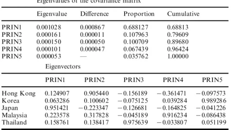
In order to determine the most important common factors that in¯uence the interest rates of countries in the Asian Paci®c, a principal component analysis is taken of the excess return on the currency deposit of those ®ve Asian Paci®c countries. The last column of Table 2 displays the total variance captured by the principal components. The ®rst two principal components explain 80% of the total variance; these components will be priced in the next sub-section. The ®rst component may be seen as a weighted
Table 2. Principal component analysis for country’s interest rate
Five Asian Paci®c countries’ interest rates: Hong Kong, Korea, Japan, Malaysia, and Thailand, are taken to form the principal components. The interest rates are the one-month interest rate of that currency compounded by the rate of change of the exchange rate relative to the US dollar, minus the dollar one-month risk-free rate.
Eigenvalues of the covariance matrix
Eigenvalue DiVerence Proportion Cumulative
PRIN1 0.001028 0.000867 0.688127 0.68813 PRIN2 0.000161 0.000011 0.107963 0.79609 PRIN3 0.000150 0.000050 0.100709 0.89680 PRIN4 0.000101 0.000047 0.067439 0.96424 PRIN5 0.000053 Ð 0.035762 1.00000 Eigenvectors
PRIN1 PRIN2 PRIN3 PRIN4 PRIN5
Hong Kong 0.124907 0.905440 70.156189 70.361471 70.097573
Korea 0.063286 0.100602 70.075125 0.039284 0.989286
Japan 0.951421 70.223347 70.126681 70.164825 70.041226
Malaysia 0.223578 0.317828 70.045189 0.916234 70.086438
Thailand 0.158761 0.138417 0.975639 70.033807 0.051199
average of the excess return of those ®ve countries’ currency deposits, where the excess return of Japan has the highest weight. This result is also supported by the work of Ferson and Harvey (1993), which used the relative shares of the total real gross domestic product (GDP) as the weights for the global in¯ation measure. In contrast to the ®rst component, the second component assign Japan a negative weight.
Testing the conditional asset pricing model
The classic APM was examined as well as the international APM. The formulations of these two models were shown in Equation 8. The foreign exchange risk was priced in the
international APM, while it was not priced in the classic APM.
Panel A of Table 3 displays the results of testing the conditional classic APM. Six countries were examined: ®ve Asian Paci®c equity markets and the USA. There are 42 orthogonality conditions and 6 parameters, which implies that there are 36 overidentifying conditions. The J test of the overidentifying restrictions has a p-value of 0.1182. Hence, this classic model was not rejected during the sample period. The time-varying world price of risk was created by the instrumental variables and the constant par-ameters. Three of the six parameters were diVerent from zero at a 5% signi®cance level. Lack of rejection implies that the conditional classic APM can still capture the
Table 3a. Estimation of the conditional classic and international APM: conditional classic APM For classic, the following equations are estimated by GMM
etˆ zt¡1¯mrmt
hitˆ rit¡ ritet For international, the following equations are estimated by GMM
etˆ XL
jˆ1
zt¡1¯jrjt‡ zt¡1¯mrmt
hitˆ rit¡ ritet
There are six equity markets, which are Hong Kong, Korea, Japan, Malaysia, Thailand, and the USA, to be examined.
Lag world Lag US Lag TB Lab bond
Parameters Constant return dividend spread spread January
Coe cient 711.072 233.990 779.274 7674.938 7731.462 71.088
(t-statistics) (71.479) (6.062)* (1.984)* (73.156)* (71.094) (70.215)
Notes: The number of orthogonality conditions ˆ 42:
The number of parameters ˆ 6:
The number of overidentifying restrictions ˆ 36: À2…36† ˆ 46:2267, p-value ˆ 0:1182:
* Signi®cance at the 5% level.
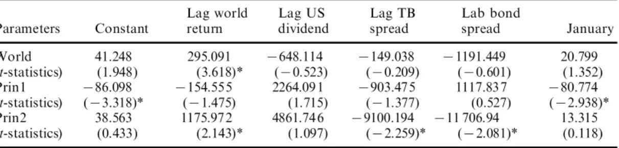
Table 3b. Estimation of the conditional classic and international APM: conditional international APM
Lag world Lag US Lag TB Lab bond
Parameters Constant return dividend spread spread January
World 41.248 295.091 7648.114 7149.038 71191.449 20.799 (t-statistics) (1.948) (3.618)* (70.523) (70.209) (70.601) (1.352) Prin1 786.098 7154.555 2264.091 7903.475 1117.837 780.774 (t-statistics) (73.318)* (71.475) (1.715) (71.377) (0.527) (72.938)* Prin2 38.563 1175.972 4861.746 79100.194 711 706.94 13.315 (t-statistics) (0.433) (2.143)* (1.097) (72.259)* (72.081)* (0.118)
Notes: The number of orthogonality conditions ˆ 42:
The number of parameters ˆ 18:
The number of overidentifying restrictions ˆ 24: À2…24† ˆ 22:5048, p-value ˆ 0:5492:
dynamics of returns on these equity markets, and is con-sistent with the ®ndings of Harvey (1991) for MSCI indices of industrialized countries.
Panel B of Table 3 displays the results of the conditional version of the internationa l APM. With 42 orthogonalit y conditions and 18 parameters, there are 24 overidentifyin g restrictions. The p-value of the J test is equal to 0.5492, which was not rejected by the data. Six of the eighteen par-ameters were distinct from zero at a 5% signi®cance level.
To compare these two models which were not rejected, a more robust test was needed for examining the existence of the prices of foreign exchange risk for the Paci®c Basin equity markets. The classic APM can be tested against the international APM because these two models are nested. Following Newey-West (1987), the international APM was estimated ®rst; then, the classic APM was esti-mated using the weighting matrix of the unconstrained model, which was the international APM. The diVerence between the constrained and unconstrained À2was distrib-uted to À2 with 12 degrees of freedom. The result is reported in Panel A of Table 4, which shows that the con-strained À2 is much higher than the unconstraine d À2. Therefore, it can be concluded that the time-varying prices of foreign exchange risk were present for the Paci®c Basin equity markets during the sample period. The empirical result was consistent with the evidence of Harvey et al. (1994) for OECD countries, where one risk premium was
not su cient to characterize the variation in expected returns, and there existed another premium, which was related to foreign exchange risk.
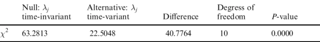
Table 4 also shows the results of testing whether the prices of market risk and foreign exchange risk are time-varying or not. In Panel B, the Newey-West test is used to examine the null hypothesis of the time-invariant world price of market risk against the alternative of a time-varying one. The hypothesis of the time-invariant world price of market risk is rejected. In Panel C, the time-invariant prices of exchange risk are also tested by the Newey-West test. The p-value, which was extremely small, rejects the null hypothesis. Again, time-varying prices of exchange risk are suitable for these Paci®c Basin equity markets. The ®nding is consistent with many empiri-cal tests, e.g., Dumas and Solnik (1995) and Engel and Rodrigues (1989).
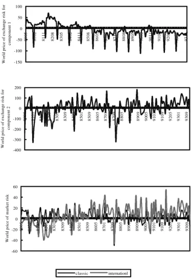
The projection of world price of risk
The evidence of time-varying world price of risk can be explained in that Paci®c Basin countries experienced many changes in their economies during the sample period, including reduced capital control, liberalized exchange rates, and high rates of economic growth. Figure 1 displays the time variations of the world prices of market risk and exchange risk, which were projected by the instrumental
Table 4a. Hypothesis test: Testing classic APM against international APM The following equations are examined by GMM and Newey-West test
etˆ XL
jˆ1
zt¡1¯jrjt‡ zt¡1¯mrmt
hitˆ rit¡ ritet
Null: Alternative: Degrees of
¯jˆ 0 at least one ¯j6ˆ 0 DiVerence freedom P-value
À2 65.1550 22.5048 42.6501 12 0.0000
Table 4b. Hypothesis test: Testing time-invariant price of market risk against time-variant
Null: ¶m Alternative: ¶m Degrees of
time-invariant time-variant DiVerence freedom P-value
À2 46.6645 22.5048 24.1597 5 0.0002
Table 4c. Hypothesis test: Testing time-invariant price of exchange risk against time-variant
Null: ¶j Alternative: ¶j Degress of
time-invariant time-variant DiVerence freedom P-value
variables. The prices of market risk under the classic and international APM vary in an almost identical fashion, but not of the same magnitude. The magnitude of volatility of the price of market risk under the classic is smaller than the international. The addition of foreign exchange risk plays an important role in estimating the price of market risk. It is interesting to observe that the world price of exchange risk is more volatile than the world price of market risk. For the world price of component 1 exchange risk, there is
a signi®cant January eVect towards negative. The negative world price of exchange risk is not surprising. Dumas and Solnik (1995) indicated that the world prices of exchange risk should be negative when the risk aversion of each investor subpopulation is greater than 1. The January eVect is more noteworthy, however.6
In the internationa l APM of Adler and Dumas (1983), they had argued that there were two hypotheses to be tested: (1) the regression coe cients, which are the prices of risk, on all the covariance terms add up to one; (2) the coe cient on the covariance with the market is positive. The prices of risk in the present model are time-varying and ¯uctuate between positive and negative values, so the aver-age value is used to inspect the values of the world price of risk. On average, the world price of market risk is positive, but all the prices of risk do not sum to one. There may be some other factors that in¯uence the risk premia in the Paci®c Basin equity markets, such as political intervention. Although most Paci®c Basin countries have had their capi-tal markets open for a long time, there still remain some limits on foreign investors under certain regulations. These restrictions may limit these markets from becoming fully integrated into the world capital market. As a result, an asset pricing model with time-varying integration may be proper to capture the dynamics of risk premia for Paci®c Basin capital markets.7
V . C O N C L U S I O N
Five Asian Paci®c as well as the US equity markets were examined by the conditional APM. A principal component analysis is taken to extract the common factors that in¯uence those Asian Paci®c interest rates. Both of classic and international APM were ex-amined, where the exchange risk was priced in the international APM and was not priced in the classic APM. The world prices of market risk and exchange risk were allowed to vary over time with common market information variables.
Using the GMM estimation and the J test, both models, classic and international, were not rejected. However, using a more robust test, the Newey-West test, the null hypoth-esis of the classic APM was rejected against the inter-national APM. Moreover, the null hypotheses of time-invariant prices of market risk and exchange risk were rejected against the time-variant . These results suggest
6The unreasonable values for the world prices of risk may result from model misspeci®cation or improper simplifying assumptions; see
Glassman and Riddick (1996).
7The test of time-varying world market integration had been explored by Bekaert and Harvey (1995). They found that a number of
emerging markets exhibit time-varying integration.
-150 -100 -50 0 50 100 80 05 81 02 81 11 82 08 83 05 84 02 84 11 85 08 86 05 87 02 87 11 88 08 89 05 90 02 90 11 91 08 92 05 93 02 93 11 W or ld p ri ce o f ex ch an ge r is k fo r c om po ne nt 1 -400 -300 -200 -100 0 100 200 80 05 81 01 81 09 82 05 83 01 83 09 84 05 85 01 85 09 86 05 87 01 87 09 88 05 89 01 89 09 90 05 91 01 91 09 92 05 93 01 93 09 W or ld p ri ce o f ex ch an ge r is k fo r c om po ne nt 2 -60 -40 -20 0 20 40 60 80 05 81 01 81 09 82 05 83 01 83 09 84 05 85 01 85 09 86 05 87 01 87 09 88 05 89 01 89 09 90 05 91 01 91 09 92 05 93 01 93 09 W or ld p ri ce o f m ar ke t r is k classic internationl
Fig. 1. The projection of the world price of risk
The time variations of the world prices of market risk and exchange risk are projected by the instrumental variables, includ-ing the world market return, the S&P500 dividend yield, the US yield spread between Moody’s Baa and Aaa bonds, the excess return on a three month bill, and a dummy variable for the month of January.
that the conditional classic APM can still capture the dynamics of the returns on the Paci®c Basin equity mar-kets, but the exchange risk should be priced to get a more explanatory power. In addition, the world prices of market risk and exchange risk are time-varying conditional on some common market information variables during the sample period.
The results imply that the exchange risk cannot be fully diversi®ed away in the Paci®c Basin equity markets. Hence, active hedging policies might be needed to gain the diver-si®ed bene®ts of investing into these markets.
A C K N O W LE D G E M E N T
The authors wish to thank the editor and an anonymous reviewer for their helpful comments and suggestions on an earlier version of this paper.
R E F E R E N C ES
Adler, M. and Dumas, B. (1983) International portfolio choice and corporation ®nance: a synthesis, Journal of Finance, 38, 925±84.
Bekaert, G. and Harvey, C. R. (1995) Time-varying world market integration, Journal of Finance, 50, 403±44.
Bessembinder, H. and Chan, K. (1995) The pro®tability of tech-nical trading rules in the Asian stock markets, Paci®c-Basin
Finance Journal, 3, 257±84.
Cumby, R. E. (1990) Consumption risk and international equity returns: some empirical evidence, Journal of International
Money and Finance, 9, 182±92.
Davidson, R. and Mackinnon, J. G. (1993) Estimation and
Inference in Econometrics, Oxford University Press, New
York.
Dumas, B. (1994) A test of the international CAPM using busi-ness cycles indicators as instrumental variables, National
Bureau of Economic Research (NBER) Working Paper
No. 4657.
Dumas, B. and Solnik, B. H. (1995) The world price of foreign exchange risk, Journal of Finance, 50, 445±79.
Engel, C. and Rodrigues, A. P. (1989) Tests of international CAPM with time-varying covariances, Journal of Applied
Econometrics, 4, 119±38.
Ferson, W. E. and Foerster, S. R. (1994) Finite sample properties of the generalized method of moments in tests of conditional asset pricing models, Journal of Financial Economics, 36, 29± 55.
Ferson, W. E. and Harvey, C. R. (1993) The risk and predictabil-ity of international equpredictabil-ity returns, Review of Financial
Studies, 6, 527±66.
Glassman, D. A. and Riddick, L. A. (1996) Why empirical inter-national portfolio models fail: evidence that model
mis-speci®cation creates home asset bias, Journal of
International Money and Finance, 15, 275±12.
Hansen, L. P. (1982) Large sample properties of generalized method of moments estimators, Econometrica, 50, 1029±54. Hansen, L. P. and Jagannathan, R. (1991) Implications of
secur-ity market data for models of dynamic economies, Journal of
Political Economy, 99, 225±61.
Harvey, C. R. (1991) The world price of covariance risk, Journal
of Finance, 46, 111±57.
Harvey, C. R. (1995) Predictable risk and returns in emerging markets, Review of Financial Studies, 8, 773±816.
Harvey, C. R., Solnik, B. and Zhou, G. (1994) What determines expected international asset returns? NBER Working Paper No. 4660.
Harvey, C. R. and Zhou, G. (1993) International asset pricing with alternative distributional speci®cations, Journal of
Empirical Finance, 1, 107±131.
Lucas, R. E. (1982) Interest rates and currency prices in a two-country world, Journal of Monetary Economics, 10, 335±60. Newey, W. K. and West, K. D. (1987) Hypothesis testing with e cient method of moments estimation, International
Economic Review, 28, 777±87.
Perold, A. F. and Schulman, E. C. (1988) The free lunch in currency hedging: Implications for investment policy and performance standards, Financial Analysts Journal, 44, 45± 50.
Phillips, P. C. B. and Perron, P. (1988) Testing for a unit root in time series regression, Biometrika, 75, 335±46.
Shapiro, S. S. and Wilk, M. B. (1965) An analysis of variance test for normality (complete samples), Biometrika, 52, 591±611. Solnik, B. H. (1974a) An equilibrium model of the international
capital market, Journal of Economic Theory, 8, 500±24. Solnik, B. H. (1974b) The international pricing of risk: An
empiri-cal investigation of the world capital market structure,
Journal of Finance, 29, 365±78.
Solnik, B. H. (1983) International arbitrage pricing theory,
Journal of Finance, 38, 449±57.
Stehle, R. (1977) An empirical test of the alternative hypotheses of national and international pricing of risky assets, Journal of
Finance, 32, 493±502.
Stulz, R. (1981) A model of international asset pricing, Journal of
Financial Economics, 9, 383±406.
Stulz, R. (1994) International portfolio choice and asset pricing: an integrative survey, NBER Working Paper No. 4645. Thomas, S. H. and Wickens, M. R. (1993) An international
CAPM for bonds and equities, Journal of International
Money and Finance, 12, 390±412.
Wheatley, S. (1988) Some tests of international equity integration,
Journal of Financial Economics, 21, 177±212.
A P P E N D I X
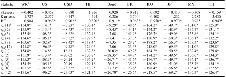
Table A1 reports some additional statistics and unit root tests for the data. The skewness statistics are almost con-sistent with symmetry, but the kurtosis statistics are signif-icant deviations from zero for most data. From the W statistic of Shapiro and Wilk (1965), only the world port-folio and Malaysia are not rejected at a 5% signi®cance level. This implies that most data are unlikely to be gener-ated from a normal distribution.
The rest of Table A1 shows the result of detecting the presence of a unit root in the data. Phillips-Perron (1988) was used to test the null hypothesis of the existence of a unit root, because this test allows weakly dependent and heterogeneously distributed errors. Most tests provide sig-ni®cant evidences of rejection of the unit root except the US dividend yield spread and bond yield spread. While the US dividend yield spread is not rejected when the test includes constant and trend terms with truncation at lag
1, 2, 3, and 4 at a 5% signi®cance level, these tests are rejected at a 10% level. The tests of the bond yield spread are not rejected when they do not include constant and trend terms with truncation at lag 3, 4, 8, and 12 at a 5%
signi®cance level, but they are also rejected at a 10% level. As a result, it is hard to conclude that these two series are generated from a random walk process. The other series could be characterized as integrated of order zero, i.e., I(0).
Table A1. Other summary statistics and unit root tests
Statistic WRa US USD TB Bond HK KO JP MY TH
Skewess 70.402 70.458 0.980 1.926 0.920 70.917 0.692 0.410 70.308 70.159 Kurtosis 1.727 2.577 0.447 4.694 0.286 3.740 0.408 1.232 2.282 3.430 Wb 0.984 0.963* 0.902* 0.820* 0.911* 0.963* 0.958* 0.970* 0.985 0.949* ½nc…1†c 7154.8* 7114.7* 78.23* 7130.1* 79.29* 7148.5* 7164.2* 7149.7* 7131.0* 7125.9* ½nc…2† 7155.9* 7113.4* 78.63* 7134.6* 78.45* 7144.1* 7174.2* 7148.9* 7135.7* 7131.1* ½nc…3† 7155.4* 7108.3* 78.62* 7132.4* 77.68 7141.9* 7176.7* 7149.0* 7135.8* 7134.1* ½nc…4† 7154.6* 7105.1* 78.62* 7127.9* 77.41 7137.0* 7180.9* 7150.3* 7136.1* 7132.2* ½nc…8† 7163.6* 7102.9* 79.42* 7119.4* 77.35 7128.2* 7198.2* 7156.3* 7138.3* 7123.6* ½nc…12† 7171.8* 796.5* 79.48* 7124.0* 77.06 7133.6* 7218.0* 7169.5* 7141.0* 7129.8* ½ct…1† 7154.8* 7114.8* 718.63 7132.3* 730.03* 7149.7* 7164.2* 7150.5* 7132.4* 7129.4* ½ct…2† 7155.9* 7113.4* 720.02 7136.8* 728.35* 7144.7* 7174.2* 7149.6* 7136.6* 7134.3* ½ct…3† 7155.3* 7108.3* 720.24 7134.2* 726.71* 7141.6* 7176.7* 7149.7* 7136.1* 7136.7* ½ct…4† 7154.5* 7105.1* 720.49 7129.1* 726.51* 7135.9* 7180.9* 7151.0* 7135.7* 7134.1* ½ct…8† 7163.5* 7102.8* 723.32* 7118.2* 727.73* 7123.6* 7198.4* 7156.6* 7135.4* 7122.5* ½ct…12† 7171.6* -96.2* 723.63* 7121.3* 726.70* 7125.6* 7218.5* 7169.2* 7135.3* 7126.4*
Notes:aWR (world portfolio), USD (US Dividend Yield), TB (Treasury Bill yield spread), Bond (bond yield spread), HK (Hong Kong), KO (Korea), JP (Japan), MY (Malaysia), and TH (Thailand).
bW statistic is based on Shapiro and Wilk (1965), which is a test of null hypothesis of normal distribution. c
½nc…1† are the Phillips-Perron test for a unit root, where nc represents non-constant and non-trend, ct denotes constant and trend, and
the number in parentheses is the lag truncation parameters. The signi®cance level is based on asymptotic critical values in Page 708 of Davidson and Mackinnon (1993).