October 2005 pp. 1-28
Capacity Utilization, Congestion and
Production Performance: An
Empirical Examination
∗
Sui-Hua Yu
†National Chung Cheng University
ABSTRACT: Increases in capital expenditures in various industries have triggered companies to make sustained efforts to manage capacity related costs. More research is being devoted to the allocation of capacity related costs and its role in incremental decision-making. To date, however, such research consists mainly in analyses of the relation between capacity utilization and cost, while the relevant empirical evidence is lacking. This study fills in this lacuna by investigating empirically the impact of capacity utilization on production performance and the moderating impact of manufacturing flexibility and manufacturing variability on the performance effect of capacity utilization. Empirical results based on six-month machine-level data from one semiconductor wafer fabrication company indicate that increased capacity utilization not only leads to longer waiting time and longer manufacturing cycle time but also causes decrease in production quality and thus increase in operating costs, with the implication that maximizing the level of capacity utilization is not necessarily optimal for firms. In addition, the empirical results reveal that performance degradation arising from high capacity utilization is greater in a production environment with higher levels of manufacturing variability. But, firms can reduce the impact of capacity utilization on production performance by improving manufacturing flexibility. This study makes the following contributions to extant research. First, it provides initial empirical evidence for congestion cost with the finding that production performance decreases with increase in capacity utilization. Second, its empirical findings relating manufacturing flexibility and manufacturing variability to performance impact of capacity utilization increase our understanding of the behavior of congestion cost
∗
The author would like to thank two anonymous reviewers for their constructive comments and suggestions. I also appreciate the input of the participants at the 2005 Accounting Theory and Practice Conference. I am especially thankful for suggestions made by Prof. Anne Wu. Financial support from the National Science Council is greatly acknowledged (Project No. NSC94-2416-H-194-031). Data support from the research company is especially appreciated.
†
Corresponding author. 168 University Rd., Min-Hsiung, Chia-Yi, Taiwan, ROC. Tel:
Keywords: Capacity utilization, Manufacturing flexibility, Manufacturing
variability,
Production performance, Semiconductor
manufacturing industry
Data Availability: The author has a confidentiality agreement with the firm
providing the data for this study. Revealing its identity and
disseminating the data are precluded without its permission.
I. INTRODUCTION
I
n recent years, the issue of allocating and managing capacity related cost has become increasingly important to the practice and management accounting research owing to rapid developments in information technology and improvements in production technology. Conventional management accounting analyses make the assumption that the opportunity cost of capacity is zero. Therefore, in a capacity-constrained environment, maximizing capacity utilization is believed to be the key to achieving cost advantage (Banker et al. 1988; McNair 1996; Cooper and Kaplan 1999). In practice, firms all dedicate themselves to reducing or eliminating unused capacity in order to improve capacity productivity and cost performance (Campbell 2004).Operations research, however, indicates that the cost of increasing capacity utilization in stochastic and congested production environments is significantly different from the cost considered in traditional management accounting analyses. Specifically, in a stochastic production environment, increasing capacity utilization increases congestion and thus causes increase in waiting time, manufacturing cycle time, inventory carrying costs and operating costs. Besides, increased cycle time and delivery delay might lead as well to lower sales price realizations (Karmarkar et al. 1985; Banker et al. 1988). Putting these factors together, the relevant cost of raising capacity utilization is actually positive, but not zero. Ignoring these costs, therefore, might lead to sub-optimal management decisions.
Congestion is widely studied in operations and production management literature, so prior studies tended to focus on strategies to eliminate congestion in the production environments by production scheduling, dispatching and plant layout decisions (for example, Connors et al. 1996; Benjaafar and Gupta 1998; Benjaafar 2002). Few analyzed the cost of congestion. In management accounting, Banker et al. (1988) was the first one to propose the concept of congestion cost. They used mathematical analysis and a single numerical example to prove the existence of congestion cost, indicating that the opportunity cost of capacity is a smooth function but not discontinuous. However, although congestion cost was investigated in several studies, empirical evidence on congestion cost remains scarce.
Balakrishnan and Soderstrom (2000) and Gupta et al. (2003) are two studies providing initial evidence for the existence of congestion cost by examining the impact of capacity utilization on performance and cost. Using data from hospitals and one printing company, they found that increased capacity utilization leads to degradation in performance and increase in operating costs. Besides, Balakrishnan and Soderstrom (2000) found that the adverse impact of capacity utilization on performance is contingent
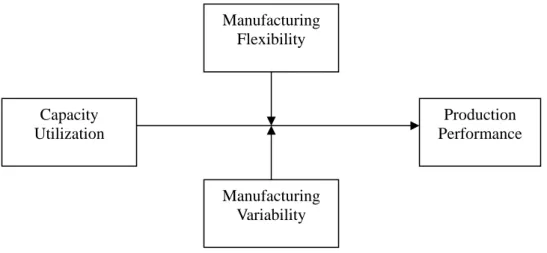
on the specifics of the process, implying that congestion cost differs in different manufacturing environments. However, they did not go on to investigate which factors drive congestion cost and in which ways congestion cost can be reduced. The understanding of the behavior of congestion cost is constrained. To fill in the gap between the extant researches, this study investigates empirically the following research questions. (1) How does capacity utilization affect production performance? (2) How does manufacturing variability affect the relationship between capacity utilization and production performance? (3) How does manufacturing flexibility affect the relationship between capacity utilization and production performance? The conceptual framework of this study is presented in Figure 1.
Figure 1: Conceptual Framework
The semiconductor manufacturing industry is technologically complex and capital- intensive. In this industry, equipment depreciation accounts for a large proportion of production cost and manufacturing strategies focus mainly on increasing capacity utilization and minimizing production cost while improving quality and delivery time performance (Uzsoy et al. 1992). However, several problems in this environment make manufacturing management more difficult and challenging. They are complex product flows, random rework, evolving process technologies, diverse equipment characteristics, and frequent machine breakdowns. These factors contribute to a highly stochastic and congested manufacturing environment, which provides an ideal setting for us to investigate the association between capacity utilization, congestion and production performance.
Analyzing six-month machine-level data obtained from one semiconductor manufacturing company, this study finds that increased capacity utilization not only leads to longer waiting time and manufacturing cycle time but also causes decrease in production quality, and thus, increase in operating costs, with the implication that maximizing the level of capacity utilization is not necessarily optimal for firms. Besides, the empirical results also indicate that performance degradation arising from high capacity utilization is greater in a production environment with higher level of
Capacity Utilization Production Performance Manufacturing Flexibility Manufacturing Variability
manufacturing variability; but firms can reduce the impact of capacity utilization on production performance by improving manufacturing flexibility. These results indicate that congestion costs increase with increase in manufacturing variability but decrease with increase in manufacturing flexibility.
The reminder of the paper is structured as follows. Literatures on capacity utilization and congestion cost are reviewed in Section II. Research hypotheses are developed in Section III. Research site and its capacity management practices are described in Section IV. In Section V, I discuss the data collection and research methodology. Empirical results are presented in Section VI. Conclusions, limitations and directions for future research are discussed in Section VII.
II. LITERATURE REVIEW
Definition and Measurement of Capacity
Capacity is the maximum workload an operating unit can handle in a production environment (Stevenson 1996) measured either by time or by output quantity. Generally speaking, there are five measurements of capacity: theoretical capacity, practical capacity, normal capacity, budgeted capacity and actual capacity. Theses five measurements differ in the assumption of available capacity. For example, theoretical capacity is the optimal amount of work that a process or plant can complete using a 24-hour, 7-day operation with zero waste. Practical capacity is the level of output generally attained by a process, which adjusts theoretical capacity downward for unavoidable nonproductive time. Actual capacity is the capacity deployed by the company for a production period, which is usually the lowest level of output among the five capacity measurements (McNair and Vangermeersch 1998). Theoretical capacity and practical capacity are the two measurements used most frequently by firms in their capacity cost management systems because the other three measurements embed too much waste in standards to help continuous improvement of capacity productivity (McNair and Vangermeersch 1998).
According to capacity management literature, it is important to analyze capacity deployment for firms while making capacity improvement decisions. Capacity deployment can be classified into three categories: productive capacity, nonproductive capacity and idle capacity. Productive capacity is capacity that provides value to the customer and results in the production of good products or services. Idle capacity is capacity currently not in use, either planned or unplanned. It may exist for management policy, marketing, contractual or legal reasons. Nonproductive capacity is capacity neither in productive state nor in idle state. It is usually an undesirable use of capacity, such as setups, unplanned maintenance, making scrap or performing rework and thus offers an opportunity for improvement. To improve capacity productivity, firms generally target idle capacity and nonproductive capacity for elimination or reduction (Klammer 1996). Understanding the sources of idle capacity and nonproductive capacity is helpful to create more productive capacity and to increase productivity further.
Congestion and Capacity Utilization Related Studies
Operations research shows that the arrival of production lots into each workstation is a stochastic process. As utilization approaches capacity limit, congestion increases and
generally causes performance degradation. Congestion, therefore, is studied widely in production management literature but the focus is mainly on strategies for eliminating or reducing congestion through management policies to achieve performance objective. For example, Connors et al. (1996) developed an open queuing network model for performance analysis of semiconductor manufacturing facilities and analyzed how to attain planned cycle times in a congested production environment. Benjaafar and Gupta (1998) investigated how to reduce manufacturing cycle time and inventory levels using flexible manufacturing strategies in a capacity-constrained environment. Benjaafar (2002) presented a model that captures the relationship between facility layout, congestion and two performance measurements, then uses this model to analyze how plant layouts help reduce manufacturing lead times and minimize work-in-process inventories. Benjaafar et al. (2004) developed a model to analyze whether product variety causes congestion and leads further to increases in inventory carrying costs.
In management accounting literature, most studies focus on examining analytically the allocation of capacity related costs and its role in incremental decision-makings (for example, Hansen and Magee 1993; Balakrishnan and Sivaramakrishnan 1996; Banker et al. 2002), but few investigated the cost of congestion empirically. Banker et al. (1988) was the first one to propose the concept of congestion cost. Using a queuing model and one numerical example, they showed that operating costs increase with increase in capacity utilization. Based on findings from Banker et al. (1988), Balakrishnan and Soderstrom (2000) and Gupta et al. (2003) provide initial empirical evidence on congestion cost. Using data from 225,473 maternity admissions at 30 hospitals in the state of Washington, Balakrishnan and Soderstrom (2000) test whether the rate of Caesarian section increases on congested days and find that congestion leads to increased Caesarian section rate only for “at risk” patients, indicating that cost of congestion is contingent on the specifics of the process. Gupta et al. (2003) collect data from one printing company in Taiwan and examine empirically the impact of capacity utilization on operating performance, revenues, costs and profitability. Their empirical results indicate that increased capacity utilization not only results in decline in production efficiency and increase in product cost but also leads to lower profit.
Although these studies show the cost of congestion, we lack understanding of the drivers of congestion cost. In fact, several operations studies reveal that congestion costs differ in different processes and environments. For example, Benjaafar and Gupta (1998) indicated that the impact of capacity utilization on cycle time is larger in manufacturing environments with a greater level of manufacturing variability. Benjaafar (1994) and Benjaafar (2002) showed that firms can reduce the adverse impact of congestion on cycle time and work-in-process inventory level by improving manufacturing flexibility and adopting plant specific layout designs, respectively. To fill in the gap between current researches and increase our understanding of the behavior of congestion cost, this study not only examines empirically the adverse impact of capacity utilization on production performance but also investigates how manufacturing variability and manufacturing flexibility affect performance impacts of capacity utilization.
III. HYPOTHESES DEVELOPMENT
resource is the only constraining factor in a production environment. To achieve the maximum throughput, bottleneck resource must be fully utilized and never be out of service because of breakdowns or lack of work. Conventional management accounting analyses also suggest that maximizing capacity utilization is the best way to minimize production cost. However, in accordance with queuing theory, maximizing capacity utilization increases congestion in the system and thus leads to increased inventory level, longer manufacturing cycle time and higher operating cots. Firms, therefore, should not only consider reduction of capacity cost but should evaluate the increase in operating costs when determining the optimal capacity utilization (Karmarker et al. 1985; Bitran and Tirupati 1989; Bitran and Morabito 1999).
From the queuing theory perspective, in a stochastic production environment, an increase in capacity utilization increases overall congestion in the production environment, thus resulting not only in queuing delays for the new product but also in increased delays for all existing products, the so-called “spillover effects”. In other words, when a facility runs close to capacity, the incremental cost of an additional order is not only its direct cost, but also the cost of externalities it imposes on other products (Balakrishnan and Soderstrom 2000). Banker et al. (1988) also indicate that costs of producing one additional lot include not only the cost of capacity consumed in the production process but also additional cost arising from increased manufacturing cycle time and queuing delay, such as higher inventory carrying cost, lower sales prices realization, cost of expediting and cost of rework.
In addition, Balakrishnan and Soderstrom (2000) documented that congestion leads to increased Caesarian section rate and thus increased operating cost based on data from 225, 473 maternity admissions at 30 hospitals in Washington state. Analytical models in operations research show consistently that congestion increases and system performance degenerates when a production system is close to its capacity constraint (Hopp and Spearman 2001). Queuing model results also show that both average waiting time per production lot and manufacturing cycle time of all products in the system increase as capacity utilization increases (Fry and Blackstone 1988; Buss et al. 1994; Bitran and Tirupati 1989). Schaffer (1981) suggests that only 5% of manufacturing lead time is value-added in a stochastic production environment because much time is wasted on waiting due to increased capacity utilization and congestion. Using data from one printing company in Taiwan, Gupta, Randall and Wu (2003) also find that capacity utilization has an adverse impact on production efficiency, quality and costs. Those discussions lead to the following hypothesis.
Hypothesis 1: Production performance decreases with the increase in capacity utilization.
As to the impact of manufacturing variability on performance impacts of increased capacity utilization, several analytical studies provide some insights. For example, Banker et al. (1988) find that the impact of capacity utilization on manufacturing cycle time is larger in a manufacturing environment with a greater level of manufacturing variability. Miller (1987) also finds that job-shop plants generally keep lower capacity utilization to buffer against higher manufacturing variability. Specifically, the level of
manufacturing variability is greater in job-shop plants, and thus the cost of congestion is larger in this production environment. To reduce operating cost and improve performance, firms usually preserve more idle capacity to deal with the manufacturing variability.
Manufacturing variability is believed to be the primary driver of nonproductive capacity. It generally comes from customer demands, supplier deliveries and production flow (Klammer 1996;Hopp and Spearman 2001). These variations mainly result from short-term scheduling decisions and the randomness in many processes. Specifically, customer variability usually arises from the uncertainties in the ordering process. The sources of customer variability include business cycles, seasonal cycles, rush orders and erratic order flows, etc. Internal variability comes from a variety of sources. The most common source is the variations in processing time and setup time. But, machine setups, unplanned maintenance, breakdowns, scrap, rework, power failure and lot sizing all contribute to increased variability in production flow, as well. Whatever the source of variability is, reducing variability is considered one of principal ways to improve operating performance on the assumption that capacity utilization remains unchanged (Banker et al. 1988; Hopp and Spearman 2001).
Using an analytical model, Benjaafar (2002) shows that operating performance is driven by system congestion, which is a function of system variability. That is, manufacturing variability in the system increases system congestion and enlarges the queuing delay. Graves and Tomlin (2003) indicate that manufacturing variability not only increases congestions at workstations but also results in floating bottlenecks, which increase scheduling complexity and manufacturing lead times. Additionally, using data from a large financial services provider, Campbell (2004) indicated that the uncertainty in timing and processing of customer service requests leads to congestions and performance degradation. Firms therefore must invest in more excess capacity to buffer against greater uncertainty while maintaining service quality. In other words, a greater level of manufacturing variability or uncertainty increases the adverse impact of capacity utilization on production performance. Hence, I formulate the second hypothesis as follows.
Hypothesis 2: The greater the manufacturing variability is, the higher the impact of capacity utilization on production performance is.
Manufacturing flexibility is another important factor moderating the relation between capacity utilization and production performance (Benjaafar 1995). Manufacturing flexibility is the ability to absorb environmental uncertainties and respond effectively to changing circumstances (Gerwin 1987; Upton 1994). It provides a firm with the capability to deal with shifts in market requirements and helps to relieve problems caused by uncertainty and dynamic environments (Boyer and Leong 1996). Therefore, firms with greater manufacturing flexibility are more able to handle uncertainties and unplanned changes arising from internal or external environments. Specifically, manufacturing flexibility enables a firm to respond to changes in customer demands more quickly, produce a variety of products more effectively and deal with breakdowns or material defects that occur in the production process more efficiently (Gerwin 1993; Upton 1995)。
Benjaafar (1994) investigated analytically the relationship between manufacturing flexibility and performance of manufacturing systems and found that performance measurements, such as part flow time and level of work-in-process inventory, are a strictly decreasing function of flexibility with fixed capacity utilization. That is, when flexibility is introduced into a system, a great improvement in performance is achieved. Furthermore, the higher the capacity utilization is, the greater the impact of manufacturing flexibility on performance improvement is. Using a mathematical model, Benjaafar (1995, 1996) analyzed the impact of machine flexibility and routing flexibility on manufacturing performance. He found that an increase in manufacturing flexibility leads to a 50% reduction of manufacturing cycle time when capacity utilization is 90% but the extent of performance improvement gradually decreases with the increase in manufacturing flexibility. Besides, he also found that the impact of manufacturing flexibility on performance is greater in a highly utilized production environment. In other words, introducing manufacturing flexibility can dramatically improve performance when capacity utilization is high. Based on findings from Benjaafar (1996), increasing one unit level of manufacturing flexibility can reduce 4.5 units of manufacturing cycle time when capacity utilization is 90% but the reduction in manufacturing cycle time shrinks to less than one unit when capacity utilization is 60%. Furthermore, Benjaafar (1995, 1996) found that performance variability is a strictly decreasing function of flexibility. That is, increasing flexibility decreases the variability in manufacturing cycle time. Benjaafar and Gupta (1998) analyzed the benefits of flexibility by comparing system performance in flexible manufacturing systems and dedicated manufacturing systems. They suggested that the adverse impact of capacity utilization is smaller in flexible manufacturing systems but larger in dedicated ones. Combining these results, manufacturing flexibility is expected to reduce the adverse impact of capacity utilization on performance. Therefore, the following hypothesis is proposed.
Hypothesis 3: The greater the level of manufacturing flexibility is, the less the impact of capacity utilization on production performance is.
IV. RESEARCH SITE
The research site is a semiconductor wafer fabrication company dedicated to IC foundry services. The semiconductor manufacturing industry is highly capital-intensive. Specifically, building one typical eight-inch foundry plant requires capital investment of over forty billion NT dollars while building one twelve-inch foundry plant requires over one hundred billion NT dollars. Besides, capital investment increases dramatically with developments in manufacturing processes. Therefore, effectively utilizing capacity is the key to achieving cost advantage in this industry.
Furthermore, the wafer fabrication industry is the most competitive industry in the world. Firms in this industry face higher operating risk than companies in other industries because the manufacturing process is highly complex and a large equipment investment is required (Wen et al. 2001; Carayannis and Alexander 2004). Therefore, to maintain competitive advantage in such a risky and competitive environment, the company under research needs not only to increase machine utilization and throughput rate continuously,
but also to shorten manufacturing cycle time and respond quickly to the volatility in customer demands.
To manage capacity effectively, the research site uses the Overall Equipment Effectiveness system (OEE hereinafter), which is used widely in the semiconductor industry (Van Zant 2000). Under this system, capacity is measured in total time available. That is, 24 hours per day, 7 days per week, 365 days per year. In addition, one OEE metric is computed. OEE actually is a multiplication of three efficiency measurements: availability efficiency, performance efficiency and quality efficiency (Murphy et al. 1996). These three measurements enable efficiency losses to be identified. These include: breakdowns, setups, reduced speed, minor stoppages, defects (or rework) and yield loss (Nakajima 1988). Since these efficiency losses are the drivers of nonproductive capacity utilization, firms can improve capacity productivity by continuously eliminating these losses.
Semiconductor manufacturing is not only an extreme capacity-constrained manufacturing environment but also one of the most variable process and product manufacturing environments in the world (Uzsoy et al. 1992; Konopka 1996). Specifically, it has the following characteristics (Thompson 1995). The manufacture of a product generally requires hundreds of process steps, and a single machine group may be utilized more than once as successive circuit layers are added. Besides, each product has its own process route. The process routings of different products differ in the types of machines visited, the sequence of machines visited, and in the process times spent on the machines (Jeng et al. 1998). During the manufacturing process, a lot usually re-enters the same process area several times, but it does not necessarily go through the same sequence of steps or visit the same set of machines, the so-called “reentrant flow”. Therefore, production planning and scheduling is quite challenging in this environment. In addition, one wafer fab usually has a variety of different machine types, which further increases the complexity of operations. Other characteristics, such as frequent equipment alignment and calibration, hot lot, rework and scrap additionally contribute to the variability in the semiconductor manufacturing environment. Congestion, therefore, is quite pervasive in the wafer fab.
Especially in boom periods1, the impact of congestion on time and delivery performance is even more significant. Because product life cycle is short in the semiconductor industry, time-to-market is an important value driver. Manufacture cycle time and delivery performance, therefore, are major determinants of customer value. Increased cycle time can lead to delivery delays and decline in customer satisfaction, thus causing lower sales price realizations. Besides, the carrying costs of inventories increase along with the increase in manufacturing cycle time. Therefore, the research site is dedicated to improving delivery and time performance while maintaining high capacity utilization. Specifically, engineers deal with congestion that occurs at the research site and improve cycle time through efficient scheduling, dispatching, plant layout and
1
According to 2003 IEK-ITIS plan made by the Industrial Technology Research Institute, capacity utilization in the wafer fabrication industry declined to 40% in the third quarter of year 2001 but has been going up ever since. By the second quarter in year 2002, capacity utilization reached 80%. Because the research period of this study spans the first two quarters in year 2002, a boom period, congestion was quite pervasive at the research site, and operations management was emphasized at that time.
increased manufacturing flexibility.
One of mechanisms used to increase manufacturing flexibility is to bundle machines that are able to perform the same operations as one group. In this way, one production lot can be assigned to several process machines in each step, so several alternate routes are available to continue producing a given set of lots in case of breakdowns; this is called “routing flexibility”. Alternative routing capability also allows for efficient scheduling and helps overcome such production interruptions as machine breakdowns, rush orders and rework. Workload across machines is then balanced and nonproductive uses of capacity, such as idling and minor stoppage can thus be reduced. Cycle time is thereby improved (Sethi and Sethi 1990)。
V. RESEARCH METHODOLOGY
Sample Selection and Data Collection
I conduct this study using data from one dedicated wafer fabrication company. The company is one of the largest semiconductor manufacturing companies in Taiwan, with approximately a 35,000 wafer capacity per fab. During the period of this study, monthly data were obtained for a period of up to six months (beginning from January 2002) for machines located in one eight-inch wafer fab. Periodic visits were made to the research company to collect data and meet with senior managers, plant managers and engineers. Data for this research were collected from multiple sources, including company internal documents, archival records and interviews.
Because this study is intended to examine the association between capacity utilization, congestion and production performance, a congested operating environment is required. The author first reviewed the field data and then spoke with the plant manger and engineers to determine the period of study2, which spanned from January to June 2002. To ensure that the empirical results are driven by specific machine types, various machine types are included in this study. The machines selected are believed to be representative of a typical machine mix in the research company. Besides, machines with zero manufacturing variability and zero capacity utilization are deleted from the sample.
Variable Measurement
Dependent Variables
Waiting Time (WAIT). This variable is computed as average waiting time before the start of operation for production lots performed by each machine.
Manufacturing Cycle Time (CYCLE). This variable is computed as average manufacturing cycle time from start to completion of the operation for production lots performed in each machine.
Production Quality (YIELD). This variable is computed as one minus the percentage
2
According to operations research, congestion is more likely to appear in an operating environment with higher capacity utilization. Field data show that average capacity utilization of the research site is 92.37% in the first six months of year 2002 and 65.9% in the latter six months of year 2002. From interviews with engineers, I also find that congestion existing in the wafer fab during January 2002 to June 2002. Therefore, the first six months of year 2002 are chosen as the research period.
of wafers scrapped in each machine.
Independent Variables
Capacity Utilization (UTIL). Capacity utilization can be measured in percentage of actual output or in the percentage of time a constrained resource is used. This study uses time-based measurement. Specifically, capacity utilization is measured as the percentage of time of a machine spent in productive and nonproductive uses. Capacity usage is tracked on a monthly basis. Productive use is the actual running time of a machine and does not include time when the machine is idle, breaking-down or getting setups for production lots. Nonproductive use is the time a machine spends in waiting, breakdown, repair and maintenance, getting setups and performing tool tests.
Manufacturing Variability (VAR). The most prevalent sources of variability in manufacturing environments include natural variability, random outages, setups, operator availability and recycling. The impact of these factors can be divided into two variability measurements: process time variability and arrival time variability (Hopp and Spearman 2001). Based on operations research, a reasonable relative measurement of the variability of a random variable is the standard deviation divided by the mean, which is called the coefficient of variation. Therefore, I use the process time coefficient of variation and arrival time coefficient of variation to measure manufacturing variability. Specifically, the process time coefficient of variation is computed as the standard deviation in lot-level process time divided by mean process time, and the arrival time coefficient of variation is computed as the standard deviation in lot-level inter-arrival time divided by mean inter-arrival time.
Manufacturing Flexibility (FLEX). According to production management literature, the manufacturing system of the semiconductor manufacturing plant is characterized by greater level of routing flexibility (Jeng et al. 1998). Therefore, one routing flexibility measurement is designed to investigate the impact of manufacturing flexibility on performance of capacity utilization. Routing flexibility is the capability of the system to use alternate processing centers to continue producing a given set of parts in spite of machine breakdowns (Sethi and Sethi 1990; Chen et al. 1992; Chandra and Tombak 1992). In this study, the number of alternate machines per processing operation is used to define routing flexibility.
Control Variables
Production Volume (LOTS). The number of production lots processed by each machine is used to capture the impact of production volume.
Product Mix Complexity. Considering the characteristics of a semiconductor manufacturing environment, I design three measurements to control the impact of product mix complexity on production performance: the number of process technologies performed, the percentage of RD lots processed, and the percentage of hot lots processed in each machine. RD lots refer to lots processed for experimental and test purposes, not for production. Hot lots refer to lots processed in first priority orders to meet special customer demands.
Empirical Models
CYCLE t =α +β1LOTS t +β2TECH t + β3HOT t + β4 RD t + β5UTIL t +β6UTIL t
*FLEX t +β7UTIL t *VAR t +β8UTIL t *ARR t +β9CYCLE t-1 + ε
(M 1)
LOTS t = the number of production lots processed in each machine in period t;
TECH t = the number of process technologies performed in each machine in
period t;
HOT t = the percentage of hot lots processed in each machine in period t;
RD t = the percentage of RD lots processed in each machine in period t;
UTIL t = the percentage of time of a machine spent in productive and
nonproductive uses in period t;
FLEX t = the number of alternate machines per processing operation in each
machine group in period t;
VAR t = process time coefficient of variation for each machine in period t;
ARR t = arrival time coefficient of variation for each machine in period t;
CYCLE t = average manufacturing cycle time from start to completion of
operation by each machine in period t;
CYCLE t-1 = average manufacturing cycle time from start to completion of
operation by each machine in period t-1.
WAIT t =α +β1LOTS t +β2TECH t + β3HOT t + β4 RD t + β5UTIL t +β6UTIL t
*FLEX t +β7UTIL t *VAR t +β8UTIL t *ARR t +β9WAIT t-1 + ε
(M 2) Where,
WAIT t = average waiting time before the start of operation of each machine in
period t;
WAIT t-1 = average waiting time before the start of operation of each machine in
period t-1.
YIELDt =α +β1LOTS t +β2TECH t + β3HOT t + β4 RD t + β5UTIL t +β6UTIL t
*FLEX t +β7UTIL t *VAR t +β8UTIL t *ARR t +β9YIELD t-1 + ε
(M 3) Where,
YIELD t = one minus the percentage of wafers scrapped in each machine in
period t;
YIELD t-1 = one minus the percentage of wafers scrapped in each machine in
period t-1.
Data Analysis Method
To test the first hypothesis, I design three empirical models, models M1, M2 and M3, and test whether the coefficient on capacity utilization is significantly different from zero. Production volume and product mix complexity that might impact production performance are all included in the models. One-period lag waiting time, manufacture
cycle time and production quality are also included in model M1, M2 and M3, respectively, to correct for the one-order serial correlation problem. The same models are used to test the second and the third hypothesis, as well. By investigating the regression coefficients on three interaction items, I analyze the moderating effects of manufacturing flexibility and manufacturing variability on performance impacts of capacity utilization.
To enhance the robustness of the empirical results, I use both linear regression models and duration models. First, OLS is used to estimate model M1 to M3 and the linear relation between capacity utilization and production performance is tested. Then, I use the duration model to test the performance impact of capacity utilization. The analysis procedure is as follows. First, an accelerated failure time model is built based on Cox (1972). Then, four probability distributions are assumed to test if cumulative inertia exists. They are exponential, Weibull, lognormal and generalized gamma distribution. Finally, Maximum Likelihood Method is used to estimate the models. By examining the coefficients on capacity utilization and three interaction items, I test if capacity utilization affects manufacturing cycle time and analyze if performance impact of capacity utilization is moderated by manufacturing flexibility and manufacturing variability.
VI. EMPIRICAL RESULTS
Descriptive Statistics
Table 1 provides descriptive statistics for capacity utilization, manufacturing flexibility, manufacturing variability and three performance measurements. On average, capacity utilization is 83.75 %, less than 100%. This indicates that idle capacity remains, even though the machines at the research site are highly utilized. Capacity usages are further analyzed. Percentage of time spent in nonproductive uses is 14.71%, indicating that about one seventh of capacity is wasted in machine breakdowns, getting setups, performing repair and maintenance and processing scrapped wafers. Percentage of idle capacity is 16.25%, indicating that about one sixth of capacity is idled because of lower customer demand. In addition, I also find that average production yield is 99.9%, showing that the production quality in the research site is extremely high. As for time performance, it takes about 112 minutes to process one production lot with each machine, and average waiting time reaches 72 minutes.
On the other hand, 1,028 production lots were processed in the research site each month during the research period. As for product mix complexity, I find that the average number of process technologies is 11, the average percentage of RD lots is 24.09 % and the average percentage of hot lots is 2.3%, indicating that product mix complexity is high at the research site and needs to be controlled while testing the performance impact of capacity utilization. Besides, product mix complexity not only arises from the variety of process technologies, but from product innovation and variation in lead times. Furthermore, I also find that one routing flexibility measurement and two manufacturing variability measurements are all larger than zero, showing that there is manufacturing flexibility and variability at the research site.
Table 1: Descriptive Statistics
Variables N Mean Std. Err Min Max
Productive capacity utilization 2539 69.334 18.966 0 100
Non-productive capacity utilization 2539 14.712 12.798 0 92
Waiting time 2539 72.035 136.779 0.010 3042.36
Manufacturing cycle time 2539 111.964 148.812 4 3090.77
Production quality 2539 0.999 0.002 0.920 1
Number of lots processed 1935 1027.880 960.184 9 6850
Number of process technologies 1935 11.413 7.108 1 62
Percentage of RD lots processed 2539 0.241 0.177 0 1
Percentage of hot lots processed 2539 0.023 0.021 0.001 0.285
Total capacity utilization 1892 83.751 16.131 4 100
Manufacturing flexibility 2539 9.717 7.057 1 29
Process time variability 2539 1.291 2.517 0.030 34.650
Arrival time variability 2517 0.443 0.310 0.059 3.357
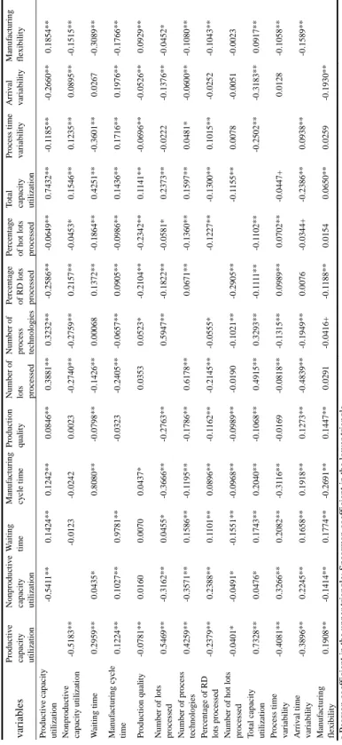
The analysis of correlation among variables is presented in Table 2. Pearson correlation coefficients are listed in the upper triangle and Spearman correlation coefficients are listed in the lower triangle. From Table 2, I find that capacity utilization is negatively correlated with production quality and positively correlated with manufacturing cycle time and waiting time. These results suggest that increased capacity utilization is associated with declines in production performance, which is consistent with the prediction. Besides, the correlation between independent variables is mostly lower than 0.7, which indicates there is no multicollinearity problem.
Impact of Capacity Utilization on Production Performance (H1)
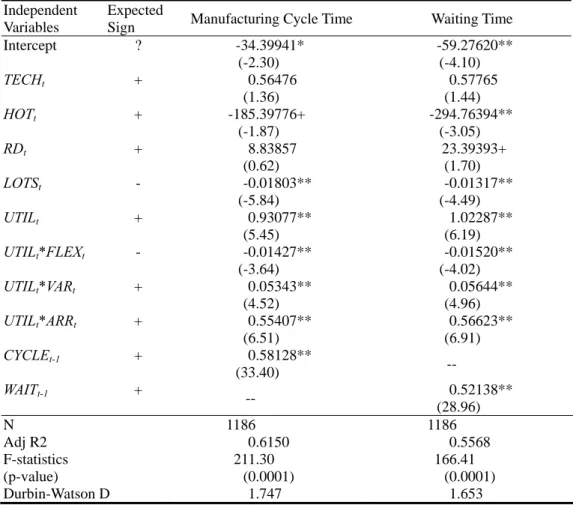
This study analyzes the impact of capacity utilization on production performance by investigating how production quality, manufacturing cycle time and waiting time change with the increase in capacity utilization. Both linear regression models and duration models are estimated. The empirical results are presented in Table 3, Table 4 and Table 5. The first hypothesis predicts that increased capacity utilization leads to declines in quality and time performance. From Table 3, each model is statistically significant at the one percent level and displays moderate to high explanatory power. In model M1, the coefficient of capacity utilization is significantly positive (coefficient = 0.9308, t-value = 5.45), indicating that, on average, it takes much longer time to process a production lot as capacity utilization increases. In model M2, I obtain similar findings. The coefficient of capacity utilization is significantly positive (coefficient = 1.0229, t-value = 6.19), as well, indicating that waiting time increases with the increase in capacity utilization.
T a ble 2 : Co rr el ation M a tr ix var ia b le s P ro d uc tiv e capac it y u ti liz atio n No n p ro d u ct iv e cap ac ity u til iz at io n W aiti n g ti m e Ma n u fa ct ur in g cy cle t im e Prod u ct ion qu a lity Nu mb er o f lot s pr o ce ss ed Numb er o f p ro ce ss te ch nol o g ie s Pe rc en ta g e of R D lot s pr o ce ss ed Pe rce n ta g e o f h o t l o ts pr o ce ss ed To ta l cap ac ity ut il iz ati o n P roc ess t im e v a ri ab il ity Ar ri v al v ar iabil ity Ma nuf ac tu ri ng fl ex ib il ity P ro d u cti v e ca pa ci ty ut il iz atio n -0 .541 1 ** 0 .1 424 ** 0 .1 242 ** 0 .0 846 ** 0 .3 881 ** 0 .3 232 ** -0 .258 6 * * -0 .064 9 ** 0 .7 432 ** -0 .1 1 8 5 ** -0 .266 0 * * 0 .1 854 ** N o npr o d u ct iv e cap ac ity u ti liz at io n -0 .518 3 * * -0 .012 3 -0 .024 2 0 .0 023 -0 .2 74 0 * * -0 .275 9 * * 0 .2 157 ** -0 .045 3 * 0 .1 546 ** 0 .1 235 ** 0 .0 8 9 5 * * -0 .151 5 ** W ai ti n g t ime 0 .2 959 ** 0 .0 435 * 0 .8 080 ** -0 .0 79 8 * * -0 .1 4 2 6 ** 0 .0 006 8 0 .1 372 ** -0 .186 4 ** 0 .4 251 ** -0 .360 1 ** 0 .0 267 -0 .308 9 ** M anuf ac tu ri ng cy cl e tim e 0 .1 224 ** 0 .1 027 ** 0 .9 781 ** -0 .0 32 3 -0 .2 40 5 * * -0 .065 7 * * 0 .0 905 ** -0 .098 6 ** 0 .1 436 ** 0 .1 716 ** 0 .1 9 7 6 * * -0 .176 6 ** Prod u ct ion qu a lit y -0 .078 1 * * 0 .0 160 0 .0 070 0 .0 437 * 0 .0 353 0 .0 523 * -0 .210 4 * * -0 .234 2 ** 0 .1 1 41 ** -0 .069 6 ** -0 .052 6 * * 0 .0 929 ** Nu m b er of l o ts pr o c es se d 0 .5 469 ** -0 .316 2 ** 0 .0 455 * -0 .366 6 * * -0 .2 76 3 * * 0 .5 947 ** -0 .182 2 * * -0 .058 1 * 0 .2 373 ** -0 .022 2 -0 .137 6 * * -0 .045 2 * Nu mb er of p roc ess te ch n o logi es 0 .4 259 ** -0 .357 1 ** 0 .1 586 ** -0 .1 1 9 5 * * -0 .1 78 6 * * 0 .6 178 ** 0 .0 671 ** -0 .136 0 ** 0 .1 597 ** 0 .0 481 * -0 .060 0 * * -0 .108 0 ** Perc en ta g e of R D lo ts pr oce ss ed -0 .237 9 * * 0 .2 388 ** 0 .1 1 01 ** 0 .0 896 ** -0 .1 1 6 2 * * -0 .2 1 4 5 ** -0 .055 5 * -0 .122 7 ** -0 .1 30 0 ** 0 .1 015 ** -0 .025 2 -0 .104 3 ** N u mb er of h o t lot s pr o c es se d -0 .040 1 * -0 .049 1 * -0 .155 1 * * -0 .096 8 * * -0 .0 98 9 * * -0 .019 0 -0 .102 1 * * -0 .290 5 * * -0 .1 1 5 5 ** 0 .0 078 -0 .005 1 -0 .002 3 T o ta l c ap ac it y ut il iz atio n 0 .7 328 ** 0 .0 476 * 0 .1 743 ** 0 .2 040 ** -0 .1 06 8 * * 0 .4 915 ** 0 .3 293 ** -0 .1 1 1 1 * * -0 .1 1 0 2 * * -0 .250 2 ** -0 .318 3 * * 0 .0 917 ** P ro ce ss time v ar iab il ity -0 .408 1 * * 0 .3 266 ** 0 .2 082 ** -0 .3 1 1 6 * * -0 .0 16 9 -0 .0 81 8 * * -0 .131 5 * * 0 .0 989 ** 0 .0 702 ** -0 .0 44 7+ 0 .0 128 -0 .105 8 ** A rr ival time v ar iab il ity -0 .389 6 * * 0 .2 245 ** 0 .1 658 ** 0 .1 918 ** 0 .1 273 ** -0 .4 83 9 * * -0 .194 9 * * 0 .0 076 -0 .034 4+ -0 .2 38 6 ** 0 .0 938 ** -0 .158 9 ** M anuf ac tu ri ng fl ex ib il ity 0 .1 908 ** -0 .141 4 ** 0 .1 774 ** -0 .269 1 * * 0 .1 447 ** 0 .0 291 -0 .041 6 + -0 .1 1 8 8 * * 0 .0 154 0 .0 650 ** 0 .0 259 -0 .193 0 * * a. P ear so n co ef fici en t in t h e u p p er t rian g le ; S p ear m an co ef fi cien t i n th e l o w er t ri an g le. b .+, * , ** = s tat ist ical ly s ig n if ic an t at th e 1 0 % , 5 % , 1 % l ev el s ( tw o -t ai led tes t) , r es p ect ively . c. A ll co rr el ati o n s ar e b as ed on p oo led d ata an d s h ou ld b e i n ter p re te d w ith c au ti o n .
Table 3: Impact of Capacity Utilization on Manufacturing Cycle Time and Waiting Time: Linear Regression Models (t-statistics in parentheses)
Note: +, *, ** = statistically significant at the 10%, 5%, 1% levels (two-tailed test), respectively.
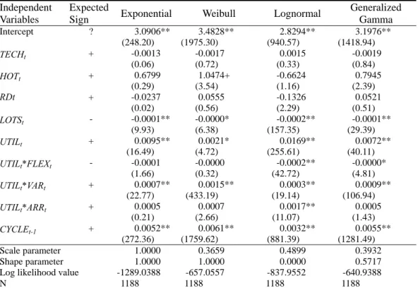
From Table 4, we see the results that generalized gamma distribution has the highest log likelihood value and exponential distribution has the lowest log likelihood value, showing that generalized gamma distribution has the highest fitness and exponential distribution has the lowest. Besides, the coefficient on capacity utilization is significantly positive across the four models, indicating that a greater level of capacity utilization leads to longer manufacturing cycle time. Put together, those results support the first hypothesis.
Independent Variables
Expected
Sign Manufacturing Cycle Time Waiting Time Intercept ? -34.39941* (-2.30) -59.27620** (-4.10) TECHt + 0.56476 (1.36) 0.57765 (1.44) HOTt + -185.39776+ (-1.87) -294.76394** (-3.05) RDt + 8.83857 (0.62) 23.39393+ (1.70) LOTSt - -0.01803** (-5.84) -0.01317** (-4.49) UTILt + 0.93077** (5.45) 1.02287** (6.19) UTILt*FLEXt - -0.01427** (-3.64) -0.01520** (-4.02) UTILt*VARt + 0.05343** (4.52) 0.05644** (4.96) UTILt*ARRt + 0.55407** (6.51) 0.56623** (6.91) CYCLEt-1 + 0.58128** (33.40) -- WAITt-1 + -- 0.52138** (28.96) N 1186 1186 Adj R2 0.6150 0.5568 F-statistics (p-value) 211.30 (0.0001) 166.41 (0.0001) Durbin-Watson D 1.747 1.653
Table 4: Impact of Capacity Utilization on Manufacturing Cycle Time: Duration Models (χ2-statistics in parentheses)
Independent Variables
Expected
Sign Exponential Weibull Lognormal
Generalized Gamma Intercept ? 3.0906** (248.20) 3.4828** (1975.30) 2.8294** (940.57) 3.1976** (1418.94) TECHt + -0.0013 (0.06) -0.0017 (0.72) 0.0015 (0.33) -0.0019 (0.84) HOTt + 0.6799 (0.29) 1.0474+ (3.54) -0.6624 (1.16) 0.7945 (2.39) RDt + -0.0237 (0.02) 0.0555 (0.56) -0.1326 (2.29) 0.0521 (0.51) LOTSt - -0.0001** (9.93) -0.0000* (6.38) -0.0002** (157.35) -0.0001** (29.39) UTILt + 0.0095** (16.49) 0.0021* (4.72) 0.0169** (255.61) 0.0072** (40.11) UTILt*FLEXt - -0.0001 (1.66) -0.0000 (0.32) -0.0002** (42.72) -0.0000* (4.81) UTILt*VARt + 0.0007** (22.77) 0.0015** (433.19) 0.0003** (19.14) 0.0009** (106.94) UTILt*ARRt + 0.0005 (0.21) 0.0007 (2.66) 0.0017** (11.07) 0.0005 (1.43) CYCLEt-1 + 0.0052** (272.36) 0.0061** (1759.62) 0.0032** (881.39) 0.0055** (1281.49) Scale parameter 1.0000 0.3659 0.4899 0.3932 Shape parameter 1.0000 1.0000 0.0000 0.5717
Log likelihood value -1289.0388 -657.0557 -837.9552 -640.9388
N 1188 1188 1188 1188
Note: +, *, ** = statistically significant at the 10%, 5%, 1% levels (two-tailed test), respectively.
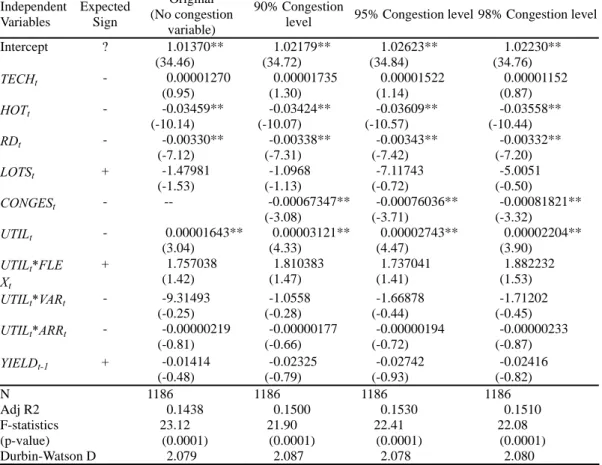
The results on the impact of capacity utilization are presented in Table 5. Each model is statistically significant at one percent level and displays moderate explanatory power. From estimation results for model M3, I find that the coefficient for the capacity utilization variable is significantly positive (coefficient = 0.00001643, t-value = 3.04), indicating that production quality increases with increase in capacity utilization. The result is contrary to the prediction of H1. After interviews and discussions with engineers, I find that the operators accumulate experience through repetitive operations and thus reduce the chance of scrapping wafers as capacity utilization increases. However, based on operations research, the probability of incurring operation errors will finally increase and production quality will finally decline as capacity utilization approaches 100%. To test whether congestion leads to lower production quality, one additional congestion variable (CONGES) is included in model M3. Empirical results are presented in Table 5, as well.
Table 5: Impact of Capacity Utilization on Production Quality (t-statistics in parentheses) Independent Variables Expected Sign Original (No congestion variable) 90% Congestion
level 95% Congestion level 98% Congestion level
Intercept ? 1.01370** (34.46) 1.02179** (34.72) 1.02623** (34.84) 1.02230** (34.76) TECHt - 0.00001270 (0.95) 0.00001735 (1.30) 0.00001522 (1.14) 0.00001152 (0.87) HOTt - -0.03459** (-10.14) -0.03424** (-10.07) -0.03609** (-10.57) -0.03558** (-10.44) RDt - -0.00330** (-7.12) -0.00338** (-7.31) -0.00343** (-7.42) -0.00332** (-7.20) LOTSt + -1.47981 (-1.53) -1.0968 (-1.13) -7.11743 (-0.72) -5.0051 (-0.50) CONGESt - -- -0.00067347** (-3.08) -0.00076036** (-3.71) -0.00081821** (-3.32) UTILt - 0.00001643** (3.04) 0.00003121** (4.33) 0.00002743** (4.47) 0.00002204** (3.90) UTILt*FLE Xt + 1.757038 (1.42) 1.810383 (1.47) 1.737041 (1.41) 1.882232 (1.53) UTILt*VARt - -9.31493 (-0.25) -1.0558 (-0.28) -1.66878 (-0.44) -1.71202 (-0.45) UTILt*ARRt - -0.00000219 (-0.81) -0.00000177 (-0.66) -0.00000194 (-0.72) -0.00000233 (-0.87) YIELDt-1 + -0.01414 (-0.48) -0.02325 (-0.79) -0.02742 (-0.93) -0.02416 (-0.82) N 1186 1186 1186 1186 Adj R2 0.1438 0.1500 0.1530 0.1510 F-statistics (p-value) 23.12 (0.0001) 21.90 (0.0001) 22.41 (0.0001) 22.08 (0.0001) Durbin-Watson D 2.079 2.087 2.078 2.080
Note: +, *, ** = statistically significant at the 10%, 5%, 1% levels (two-tailed test), respectively.
To design the congestion variable, I first review the field data and find that machines with utilization equal to or higher than 95% account for 20% of the whole sample. So, I label the machines with capacity utilization lower than 95% as “non-congested” and those with 95% or higher capacity utilization as “congested”. Then, I design the congestion variable as a dummy. For non-congested machines, the congestion variable is zero. As for congested machines, the congestion variable is one. Finally, I include the congestion variable in the model M3 and re-estimate the model. From Table 5, the model with congestion variable displays a higher explanatory power. In addition, the coefficient of congestion is significantly negative (coefficient = -0.00076036, t-value = -3.71), indicating that congestion has a negative impact on production quality, which is consistent with the prediction of H1. To examine whether the results are driven by the definition of the congestion variable, I further use 90% and 98% as cutoff points to define “congestion” respectively and estimate the model again. Empirical results are all shown in Table 5. From Table 5, we find that the coefficient of congestion is consistently negative across models with different definitions of congestion, indicting that a greater
level of capacity utilization does lead to lower production quality. The first hypothesis is supported.
Impact of Manufacturing Variability and Manufacturing Flexibility on
Performance Effects of Capacity Utilization (H2, H3)
From Table 3, I find that the coefficient of interaction between capacity utilization and process time variability is significantly positive (coefficient = 0.05343,t-value = 4.52) and the coefficient of the interaction between capacity utilization and arrival time variability is significantly positive, as well (coefficient = 0.55407,t-value = 6.51), in model M1, indicating that the impact of capacity utilization on manufacturing time increases with the increase in manufacturing variability. In addition, in model M2, I also find that the coefficient of the interaction between capacity utilization and process time variability is significantly positive (coefficient = 0.05644,t-value = 4.96) and the coefficient of the interaction between capacity utilization and arrival time variability is significantly positive, as well (coefficient = 0.56623,t-value = 6.91), indicating that increased capacity utilization leads to a greater increase in waiting time as manufacturing variability is larger. Considering the nonlinear relation between capacity utilization and production performance, I estimate the duration models and provide additional empirical evidence on the moderating effect of manufacturing variability in Table 4. From Table 4, we also find a significantly positive coefficient of the interaction between capacity utilization and manufacturing variability. These results consistently corroborate the predictions of the second hypothesis. As for the analysis of production quality, the results are shown in Table 5. From Table 5, I find that the interactions between capacity utilization and two manufacturing variability measurements both are negative (coefficient = -9.31493, -0.00000219 respectively) but do not reach a statistically significant level, indicating that manufacturing variability does not significantly affect the relation between capacity utilization and production quality.
The results for the impact of manufacturing flexibility are also shown in Table 3, Table 4 and Table 5. From Table 3, I find that the coefficient of the interaction between capacity utilization and manufacturing flexibility is significantly negative (coefficient = -0.01427,t-value = -3.64) in model M1, implying that the impact of capacity utilization on manufacturing cycle time decreases with the increase in manufacturing flexibility. That is, manufacturing flexibility helps to mitigate adverse impact of capacity utilization on production performance. Model M2 yields similar findings. The coefficient of the interaction between capacity utilization and manufacturing flexibility is significantly negative (coefficient = -0.01520,t-value = -4.02), indicating that the greater the level of manufacturing is, the smaller the impact of capacity utilization on waiting time is. Further analysis of moderating effect of manufacturing flexibility is presented in Table 4. The results show that the coefficient of the interaction between capacity utilization and manufacturing flexibility is consistently negative across models with four different probability distribution assumptions. For the two models with higher fitness in particular, the coefficient is significantly negative, showing that manufacturing flexibility reduces the adverse impact of capacity utilization on time performance. The results support the third hypothesis. As for model M3, the interaction between capacity utilization and
manufacturing flexibility is positive (coefficient = 1.757038, t-value = 1.42), supporting the prediction of H3. But, for the coefficient which is not statistically significant, the moderating effect of manufacturing flexibility on the relation between capacity utilization and production quality is not empirically validated.
VII. CONCLUSIONS AND DISCUSSIONS
This study examines the impact of capacity utilization on waiting time, manufacturing cycle time and production quality and further investigates whether manufacturing flexibility and manufacturing variability affect the performance impact of capacity utilization in the context of semiconductor manufacturing. Empirical results indicate that increased capacity utilization not only leads to longer waiting time and longer manufacturing cycle time but also causes decreases in production quality, thus increasing operating costs, with the implication that maximizing the level of capacity utilization is not necessarily optimal for firms. Besides, empirical results also indicate that performance degradation arising from high capacity utilization is greater in a production environment with higher level of manufacturing variability. Still, firms can reduce the impact of capacity utilization on production performance by improving manufacturing flexibility.
This analysis makes the following contributions to extant research. First, this study provides empirical evidence on congestion cost, indicating that production performance decreases with increase in capacity utilization in semiconductor manufacturing. Second, as far as I know, this study is the first one to analyze empirically the drivers of congestion cost. The empirical findings relating manufacturing flexibility and manufacturing variability to performance impact of capacity utilization contribute to our understanding of the behavior of congestion cost. Specifically, manufacturing variability increases the extent of performance degradation arising from increased capacity utilization, thus increasing the cost of congestion. As for manufacturing flexibility, it is beneficial for firms to reduce the adverse impact of capacity utilization on performance, thus reducing the cost of congestion. Finally, previous studies often ignored the impact of manufacturing variability and flexibility while analyzing capacity-related costs. This study finds that opportunity cost of capacity production might be under- or over-estimated without considering these two factors, causing capacity utilization decisions to be made sub-optimally.
Empirical analyses of this study also have a number of implications for management, as well. First, I find that manufacturing cycle time of each production lot with each machine increases by about one minute as capacity utilization increases by 1 %. On average, producing one production lot requires three hundred production steps. Manufacturing cycle time of one production lot will thus increase about five hours if the capacity utilization increases 1 %. Furthermore, congestion of front-end machines will result in increasing variability of back-end machines and thus increase the complexity of scheduling and cause an even greater production delay. These results suggest that managing capacity effectively is the key to achieving superior delivery performance in the semiconductor-manufacturing environment. Besides, they shed light on the importance of understanding congestion cost for capacity planning, scheduling and order acceptance decisions.
Specifically, as to production planning decisions, this study finds that increased capacity utilization leads to congestion, thus causing decrease in production performance, with the implication that maximizing the level of capacity utilization is not necessarily optimal for firms and keeping excess capacity might rather be helpful to reduce costs. For production scheduling decisions, this study finds that a greater level of capacity utilization usually results in the degradation of delivery and time performance. These results suggest that firms would better operate at a level of capacity utilization below 100 %, maintain buffer capacity and manage schedules to smooth utilization across machines. For order acceptance decisions, this study suggests that costs of decreased quality and time performance resulting from accepting additional orders or rush orders must be considered while determining optimal product mix.
In addition, this study finds that capacity utilization has a greater impact on production performance at workstations with a higher level of manufacturing variability. These results suggest that firms can either keep greater capacity slack and higher work-in-process level to buffer against manufacturing variability or reduce the level of manufacturing variability, if they would like to improve performance in a capacity-constrained environment. Finally, the empirical results indicate that manufacturing flexibility is helpful in solving congestion problems and improving time and quality performance. Therefore, firms can achieve high capacity utilization and production performance level simultaneously through increasing their manufacturing flexibility.
Limitations
This study has several limitations. Since the data are collected from a single company, the results of the empirical analysis are driven by the specific economics of the research site; thus, the generalizability of the findings is inevitably constrained. However, the research site is representative of other companies in the semiconductor manufacturing industry and congestion cost is present anytime a firm makes capacity-related decisions. Hence, I believe that several aspects of this study’s findings are germane to other companies and other industrial settings. Besides, Itter and Larcker (2001) indicate that field studies can provide a deeper analysis of management practice and contribute to theory development despite that they often have low external validities. Another limitation pertains to data availability. Since data linking the responsible scheduling and maintenance engineers to each machine is not available, I cannot investigate the impact of preventive and maintenance policies and scheduling performance on capacity utilization. Since performance in preventive and maintenance policy and scheduling policy are not systematically correlated with capacity utilization, the robustness of the empirical results is not affected. But, readers still need to exercise caution in generalizing the results of this study.
Future Studies
Future studies can test if the impact of capacity utilization on production performance is driven by other factors, such as organizational characteristics. Besides, this study focuses on the costs of congestion. Operations research indicates that higher capacity utilization can also increase revenues through processing more customer orders.
Future researches are needed to investigate the impact of capacity utilization on revenue, production cost and operating cost, thus to offer insight for determining the optimal level capacity utilization in the face of conflicting cost and revenue implications.
REFERENCES
Balakrishnan, R., and N. S. Soderstrom. 2000. The cost of system congestion: Evidence from the healthcare sector. Journal of Management Accounting Research 12, 97-114.
————, and K. Sivaramakrishnan. 1996. Is assigning capacity costs to products really necessary for capacity planning? Accounting Horizons 10, 1-11.
Banker, R. D., S. M. Datar, and S. Kekre. 1988. Relevant costs, congestion and stochasticity in production environments. Journal of Accounting and Economics 10, 171-197.
————, I. Hwang, and B. K. Mishra. 2002. Product costing and pricing under long-term capacity commitment. Journal of Management Accounting Research 14, 79-97.
Benjaaffar, S. 1994. Models for performance evaluation of flexibility in manufacturing systems. International Journal of Production Research 32, 1383-1402.
————. 1995. Effect of routing and machine flexibility on manufacturing performance.
International Journal of Integrated Manufacturing 8, 265-279.
————. 1996. Modeling and analysis of machine sharing in manufacturing systems.
European Journal of Operational Research 91, 56-73.
————. 2002. Modeling and analysis of congestion in the design of facility layouts.
Management Science 48, 679-704.
————, J. Kim, and N. Vishwanadham. 2004. On the effect of product variety in production-inventory systems. Annuals of Operations Research 126, 71-101. Benjaafar, R., and D. Gupta. 1998. Scope versus focus: issues of flexibility, capacity and
number of production facilities. IIE Transactions 30, 413-425.
Bitran, G., and R. Morabito. 1999. An overview of tradeoff curves in manufacturing systems design. Production and Operations Management 8, 56-75.
————, and D. Tirupati. 1989. Tradeoff curves, targeting and balancing in manufacturing queuing networks. Operations Research 37, 547-564.
Boyer, K. K., and G. K. Leong. 1996. Manufacturing flexibility at the plant level. Omega,
International Journal of Management Science 24, 495-510.
Buss, A., Lawrence, S. and D. Kropp. 1994. Volume and capacity integration in facility design. IIE Transactions 26, 36-47.
Campbell, D. 2004. Relevant costs, uncertainty, and supply of excess capacity in services: Theoretical analysis and empirical evidence. Working Paper.
Carayannis, E. G., and J. Alexander. 2004. Strategy, structure, and performance issues of precompetitive R&D consortia: insights and lessons learned from SEMATECH.
IEEE Transactions on Engineering Management 51, 226-232.
Chandra, P., and M. Tombak. 1992. Models for the evaluation of routing and machine flexibility. European Journal of Operational Research 60: 156-165.
Manufacturing Flexibility. Omega 20, 431-443.
Connors, D., G. Feigin, and D. Yao. 1996. A queueing network model for semiconductor manufacturing. IEEE Transactions on Semiconductor Manufacturing 9, 412-427. Cooper, R., and R. Kaplan. 1999. The Design of Cost Management Systems. NJ: Prentice
Hall.
Cox, D. R. 1972. Regression models and life-tables. Journal of Royal Statistical Society 34(2): 187-220.
Fry, T. D. and J. H. Blackstone. 1988. Planning for idle time: a rationale for the underutilization of capacity. International Journal of Production Research 26, 1853-1959.
Gerwin, D. 1987. An agenda for research on the flexibility of manufacturing processes.
International Journal of Operations and Production Management 17, 38-49.
————. 1993. Manufacturing flexibility: A strategic perspective. Management Science 39, 395-410.
Goldratt, E., and J. Cox. 1986. The Goal: A Process of Ongoing Improvement. North River Press.
Graves, S., and B. Tomlin. 2003. Process flexibility in supply chains. Management
Science 49, 907-919.
Gupta, M., T. Randall, and A. Wu. 2003. The economic impact of congestion and capacity utilization: an empirical examination. Working Paper.
Hansen, S. C., and R. P. Magee. 1993. Capacity cost and capacity allocation.
Contemporary Accounting Research 9, 635-660.
Hopp and Spearman. 2001. Factory Physics: Foundations of Manufacturing Management. Irwin publishing.
Ittner C. D., and D. F. Larcker. 2001. Assessing empirical research in managerial accounting: A value-based management perspective. Journal of Accounting and
Economics 32, 349-
Jeng, M., X. Xie, and S. Chou. 1998. Modeling, qualitative analysis, and performance evaluation of the etching area in an IC wafer fabrication system using Petri Nets.
IEEE Transactions on Semiconductor Manufacturing 11, 358-373.
Karmarkar, U. S., S. Kekre, S. Kekre, and S. Freeman. 1985. Lot-sizing and lead time performance in a manufacturing cell. Interfaces 15, 1-9.
Klammer, T. 1996. Capacity Measurement and Improvement. CAM_I study: Times Mirror.
Konopka, J. M. 1996. Improving output in semiconductor manufacturing environments. Ph. D Thesis of Arizona State University.
McNair, C. J. 1996. The Hidden Costs of Capacity. Handbook of Cost Management. Warren, Gorham & Lamont. Boston, MA.
————, and R. Vangermeersch. 1998. Total Capacity Management. St. Lucie Press. Miller, S. M. 1987. Impacts of industrial robotics: potential effects on labor and costs
within the metalworking industries. University of Wisconsin Press, Madison, WI. Murphy, R., P. Saxena, and W. Levinson. 1996. Use OEE; don’t let OEE use you.
Semiconductor International 19, 125-132.
Nakajima, S. 1988. Introducing to TPM: Total Productive Maintenance. Cambridge, Mass: Productivity Press.
Schaffer, G. H. 1981. Implementing CIM. Special Report #736. American Machinist. Sethi A., and S. Sethi. 1990. Flexibility in manufacturing: a survey. The International
Journal of Flexible Manufacturing Systems 7, 289-328.
Stevenson, W. J. 1996. Production/Operations Management. Irwin.
Thompson, M. 1995. Using simulation-based finite capacity planning and scheduling software to improve cycle time in front end operations. Proceedings of the 1995 IEEE/SEMI Advanced Semiconductor Manufacturing Conference.
Upton, D. 1994. The management of manufacturing flexibility. California Management
Review 36, 72-89.
————. 1995. What really makes factories flexible? Harvard Business Review July-Aug, 74-84.
Uzsoy, R., C. Lee, and L. Martin-Vega. 1992. A review of production planning and scheduling models in the semiconductor industry--Part one: System characteristics, performance evaluation and production planning. IIE Transactions 24, 47-60. Van Zant, P. 2000. Microchip Fabrication: A Practical Guide to Semiconductor
Processing 4th
ed. McGraw-Hill.
Wen, H., L. Fu, and S. Huang. 2001. Modeling, scheduling, and prediction in wafer fabrication systems using queueing Petri net and genetic algorithm. Proceedings of the 2001 IEEE International Conference on Robotics and Automation, Seoul, Korea.