超寬頻多輸入多輸出系統模型之建構與量測

全文

(1)國立交通大學電信工程學系碩士論文超寬頻多輸入多輸出系統模型之建構與量測 Modeling and Measurement of UWB MIMO Radio Channels. 研究生：蔡孟勳指導教授：唐震寰博士. 中. 華. 民. 國九十四年十月 I.

(2) 超寬頻多輸入多輸出系統模型之建構與測量 Modeling and Measurement of UWB MIMO Radio Channels 研究生：蔡孟勳. Student :. Mun-Xuin Tsai. 指導教授：唐震寰. Advisor : Dr. Jenn-Hwan Tarng. 國立交通大學電信工程學系碩士班碩士論文. A Thesis Submitted to Department of Communication College of Engineering National Chiao Tung University in Partial Fulfillment of the Requirements for the Degree of Master of Science in Communication Engineering October 2005 Hsinchu, Taiwan, Republic of China. 中華民國九十四年十月 II.

(3) 超寬頻多輸入多輸出系統模型之建構與量測. 研究生：蔡孟勳. 指導教授：唐震寰博士國立交通大學. 電信工程學系碩士班摘要近幾年高傳輸速率特別受到重視，例如第三代行動通訊的標準如 WCDMA 和 UWB。基於需要較高的傳輸速率，我們結合 UWB 和 MIMO 的特性。本論文介紹在 UWB MIMO 系統中，傳播環境中的傳輸端與接收端的距離、本地散射體、相鄰的天線間距及天線的擺放方式對通道容量及相關性的影響。此外在本論文中也提出了適用於室內 UWB MIMO 的通道模型，此通道模型主要是先找出 UWB 的特性再根據 802.11n 通道模型去做結合的動作。在本論文中，吾人發現了下列幾個現象：(1)在具有雜亂回波的環境下，在不同的接收距離下並不會對通道容量有任何影響; (2)在有本地散射體的環境下，通道容量會高於沒有本地散射體的環境; (3)通道容量會隨著天線單元間距的增加而增加，但在超過 0.5 波長後，天線單元間距對於通道容量就沒有顯著的影響; (4)在直接波存在的情況下，天線的擺放方式對通道容量是有影響的; (5)因為高相關性所造成的通道容量損失，會隨著 SNR 的增加而獲得補償; (6)在採用 S-V 模型的 UWB 系統中，可觀察到在直接波存在的情況下，參數Γ衰減的比沒有直接波存在的情況快; (7) 我們發展的室內 UWB MIMO 通道模型，經由與量測結果的比較結果發現我們的通道模型是可適用於 UWB MIMO 系統。 III.

(4) Modeling and Measurement of UWB MIMO Radio Channels Student：Mun-Xuin Tsai. Advisor：Dr. Jenn-Hwan Tarng. Department of Communication Engineering National Chiao Tung University Abstract. Recent years have seen the emergence of high data rate, third generation wideband wireless communication standards like wideband code division multiple access (W-CDMA) and UWB radio. Motivated by the ever increasing demand for higher wideband wireless data rates, we consider multiple antenna communication over the UWB wireless channel (UWB-MIMO). In this thesis, we will introduce the capacity and correlation properties of UWB-MIMO channels and analyze the measured UWB-MIMO channel data to investigate the effects of propagation range, local scatterer, antenna spacing and array orientation effect. And in order to propose a set of channel models applicable to indoor UWB-MIMO systems. We first present the characterization of UWB channels for indoor environment with above measured data. Then we base on 802.11n channel model to develop the UWB-MIMO channel model. In this research, some phenomena are revealing and listed as following (1) Propagation distance effect: Capacity is independent of Tx-Rx distance in the LOS/NLOS with heavy clutter. (2) Local scatterers effect: In the environment with local scatterers, the capacity is higher than the environment without local scatterers under LOS and NLOS condition. (3) Antenna spacing effect: The UWB-MIMO capacity increases as the antenna spacing increases and it saturates when the spacing is larger than 0.5λ. (4) IV.

(5) Antenna array orientation effect: Capacity for perpendicular antenna array is higher than parallel antenna array in LOS condition. But in NLOS condition, capacity is higher for perpendicular antenna array in a guided environment. (5) Capacity Loss: The relative channel capacity loss due to the effect of high antenna correlation is reduced as SNR increases. (6) From the parameter of S-V model in UWB radio channel model, we can see that Γ decay faster in the LOS condition than in the NLOS condition. (7) The UWB-MIMO channel model has been proved to be effective and accurate.. V.

(6) 誌謝首先，我要對我的指導教授唐震寰老師致上最誠摯的感謝，感謝老師在我碩士兩年的研究生涯中，給于我最細心與凡心的指導與叮嚀，並帶領我一窺無線通訊領域研究的奧妙。其次，對於波散射與傳播實驗室的學長與同學們也要致上我深深的謝意，他們所給予我在知識上和精神上的啟示與鼓勵以及在實驗量測中的協助，對完成本篇論文有莫大的助益。最後，要感謝的是我最親愛的父母親由於他們給予我的支持與關懷，使我在人生的過程裡得到最細心的呵護與照顧，讓我在成長與求學的過程中能夠有所依靠。僅以此篇論文獻給所有關心我的人。. 蔡孟勳國立交通大學，新竹市中華民國九十四年十月. VI.

(7) Table of Contents TABLE OF CONTENTS............................................................................................................................... VII TABLE CAPTIONS ......................................................................................................................................... X FIGURE CAPTIONS ......................................................................................................................................XI CHAPTER 1 ..................................................................................................................................................... 1 INTRODUCTION ............................................................................................................................................... 1 1.1 Paper review ........................................................................................................................................ 1 1.2 Motivation ............................................................................................................................................ 3 1.3 Purpose ................................................................................................................................................ 3 1.4 Organization ........................................................................................................................................ 3 CHAPTER 2 ..................................................................................................................................................... 6 FUNDAMENTAL THEORY OF UWB-MIMO SYSTEMS .................................................................................... 6 2.1 Generalized UWB-MIMO capacity formula ........................................................................................ 6 2.2 Complex Spatial Correlation Coefficient ............................................................................................. 8 2.3 Effective Degrees of Freedom (EDOF) ................................................................................................ 9 CHAPTER 3 ................................................................................................................................................... 11 MEASUREMENT SYSTEM AND ENVIRONMENT ............................................................................................. 11 3.1 Measurement System and Setup ......................................................................................................... 11 3.2 The Description of Measurement Environment .................................................................................. 14 CHAPTER 4 ................................................................................................................................................... 21 PROPAGATION, ARRAY ARRANGEMENT AND BANDWIDTH ON UWB-MIMO CAPACITY AND CHANNEL CORRELATIONS ............................................................................................................................................. 21. VII.

(8) 4.1 UWB-MIMO capacity, EDOF and correlations evaluation ............................................................... 21 4.2 Propagation Range Effect (Scenarios I/II/III/IV) ............................................................................... 22 4.2.1 LOS with light/heavy clutter (scenarios I/II)................................................................................................22 4.2.2 NLOS with light/heavy clutter (scenarios III/IV).........................................................................................25. 4.3 Local Scatterer Effect (Scenarios I/II/III/IV)...................................................................................... 28 4.4 Antenna Spacing Effect (Scenarios I/II/III/IV) ................................................................................... 33 4.5 Array Orientation Effect..................................................................................................................... 36 4.5.1 Measured results in the scenarios V and VI (corridor, site E) ......................................................................36 4.5.2 Measured results in the scenarios II and IV (laboratory, site F) ...................................................................41. 4.6 Capacity Loss..................................................................................................................................... 46 4.6.1 Capacity Loss for different antenna spacing ................................................................................................46 4.6.2 Capacity loss for different Tx-Rx distance in LOS condition...............................................................48. 4.7 Bandwidth Effect ................................................................................................................................ 50 CHAPTER 5 ................................................................................................................................................... 51 CHARACTERIZATION OF UWB CHANNELS FOR INDOOR ENVIRONMENT ..................................................... 51 5.1 Radio Channel Model ........................................................................................................................ 51 5.2 Model Parameters from the Data....................................................................................................... 53 5.2.1 Cluster and Ray Power-Decay Time Constants, Γ and γ ..............................................................................53 5.2.2 Cluster and Ray Arrival Rates, Λ and λ .....................................................................................................53. 5.3 Measured results in the Scenarios I, II, III, and IV ............................................................................ 54 5.4 Analysis of Measured results.............................................................................................................. 58 CHAPTER 6 ................................................................................................................................................... 59 HYBRID UWB MIMO CHANNEL MODEL ...................................................................................................... 59 6.1 SISO UWB Models ............................................................................................................................. 60. VIII.

(9) 6.2 UWB-MIMO Matrix Formulation...................................................................................................... 61 6.3 Cluster Modeling Approach ............................................................................................................... 63 6.3.1 PDP Shape....................................................................................................................................................63 6.3.2 PAS Shape....................................................................................................................................................63 6.3.3 Mean AOA (AOD) of Each Cluster .............................................................................................................63 6..3.4 AS of Each Cluster......................................................................................................................................64 6.3.5 Doppler Spectrum ........................................................................................................................................66. 6.4 Simulated UWB-MIMO Channel Properties Using Matlab Program................................................ 67 CHAPTER 7 ................................................................................................................................................... 71 CONCLUSION ................................................................................................................................................. 71 REFERENCE ................................................................................................................................................ 74. IX.

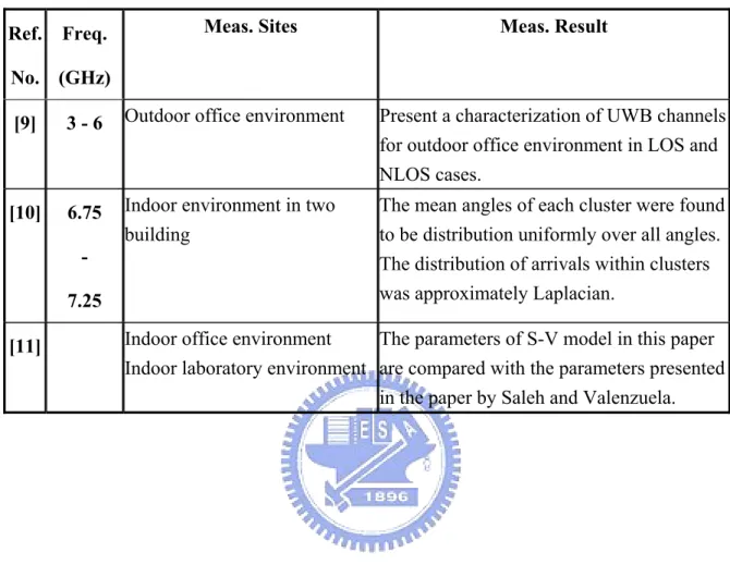
(10) Table Captions TABLE 1 SUMMARY OF RELATED WORKS ON MIMO/UWB-MIMO CAPACITY PREDICTION AND MEASUREMENT ....................................................................................................................................... 4. TABLE 2 SUMMARY OF RELATED WORKS ON UWB RADIO CHANNEL MODELING.................................................. 5 TABLE 3 SUMMARY OF RELATED WORKS ON MIMO/UWB MIMO RADIO CHANNEL MODELING ......................... 5 TABLE 4 THE MAIN PARAMETERS IN THE MEASUREMENT.................................................................................... 12 TABLE 5 MEASUREMENT SITES ........................................................................................................................... 20 TABLE 6 SUMMARY OF FOUR PARAMETERS OF S-V MODEL FOR SCENARIOS I, II, III AND IV............................... 58 TABLE 7 PARAMETERS OF PATH LOSS MODEL ...................................................................................................... 61 TABLE 8 MEAN AND STANDARD DEVIATION OF CLUSTER RMS DELAY SPREADS FOR EACH MODEL .................. 65 TABLE 9 CAPACITY OF OUR SIMULATED MODEL, 802.11N CHANNEL MODEL AND MEASURED RESULTS ............... 70. X.

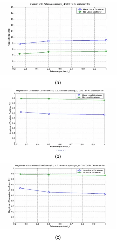
(11) Figure Captions FIG. 3-1 BLOCK DIGRAM OF THE MEASURED SYSTEM ......................................................................................... 13 FIG. 3-2 A PHOTO OF THE FREQUENCY DOMAIN CHANNEL SOUNDING SYSTEM .................................................... 13 FIG. 3-3 A PHOTO OF THE UWB ANTENNA. ......................................................................................................... 14 FIG. 3-4 FLOOR LAYOUT OF THE MEASUREMENT SITES st. (A) SITE A ON 1. (B) SITE B ON 2. FLOOR OF THE MISRC.............................................................................................. 16. nd. FLOOR OF THE MISRC ............................................................................................. 16. (C) SITE C ON LAB 213 OF THE MISRC ................................................................................................... 17 (D) SITE D ON 2 (E) SITE E ON. nd. 7 th. FLOOR OF THE 4TH ENGINEERING BUILDING ........................................................... 17 FLOOR OF THE MISRC .............................................................................................. 18. (F) SITE F ON LAB 810 OF THE MISRC .................................................................................................... 18 FIG. 3-5 RECEIVER ANTENNA BROADSIDE (A) PERPENDICULAR (ORIENTATION I) ............................................ 19 (B) PARALLEL TO THE DIRECT PATH (ORIENTATION II).............................................................................. 19 FIG 4-1 MEASURED RESULTS AT SITE B (IN LOS CONDITION IN SCENARIO I) ...................................................... 23 (A) CAPACITY VERSUS DISTANCE; (B)EDOF VERSUS DISTANCE; ............................................................... 23 (C) ρ Tx. (D) ρ Rx. VERSUS DISTANCE;. VERSUS DISTANCE.................................................................. 23. FIG 4-2 MEASURED RESULTS AT SITE C (IN LOS CONDITION IN SCENARIO II) ..................................................... 24 (A) CAPACITY VERSUS DISTANCE; ( C). ρ Tx. (B) EDOF VERSUS DISTANCE; .................................................... 24. VERSUS DISTANCE;. ρ Rx. (D). VERSUS DISTANCE; ..................................................... 24. FIG 4-3 MEASURED RESULTS AT SITE A (IN NLOS CONDITION IN SCENARIO III) ................................................. 26 (A) CAPACITY VERSUS DISTANCE; (B) EDOF VERSUS DISTANCE; .............................................................. 26 ( C). ρ Tx. VERSUS DISTANCE;. (D ). ρ Rx. VERSUS DISTANCE.................................................................. 26. FIG 4-4 MEASURED RESULTS AT SITE C (IN NLOS CONDITION IN SCENARIO IV)................................................. 27 (A) CAPACITY VERSUS DISTANCE; (B) EDOF VERSUS DISTANCE; ............................................................ 27 ( C). ρ Tx. VERSUS DISTANCE;. (D). ρ Rx. VERSUS DISTANCE .............................................................. 27. FIG. 4-5 LOCAL SCATTERERS DISCUSSION UNDER LOS CONDITION IN SITE D (SCENARIOS I/II) .......................... 29 (A) CAPACITY (B). ρ Tx. ( C). ρ Rx. VERSUS ANTENNA SPACING AT TX-RX DISTANCE=3M. ..................... 29. FIG. 4-6 LOCAL SCATTERERS DISCUSSION UNDER LOS CONDITION IN SITE D (SCENARIOS I/II) (A) CAPACITY (B). ρ Tx. ( C). ρ Rx. VERSUS ANTENNA SPACING AT TX-RX DISTANCE=7M ..................... 30. FIG. 4-7 LOCAL SCATTERERS DISCUSSION UNDER NLOS CONDITION IN SITE D (SCENARIOS III/IV)................... 31 (A) CAPACITY (B). ρ Tx. ( C). ρ Rx. VERSUS ANTENNA SPACING AT TX-RX DISTANCE=3M. ..................... 31. FIG. 4-8 LOCAL SCATTERERS DISCUSSION UNDER NLOS CONDITION IN SITE D (SCENARIOS III/IV)................... 32 (A) CAPACITY (B). ρ Tx. ( C). ρ Rx. FIG. 4-9 (A) CAPACITY (B) ρ Tx (C) ρ Rx. VERSUS ANTENNA SPACING AT TX-RX DISTANCE=7M. ..................... 32. VERSUS ANTENNA SPACING IN LOS CONDITION .................................. 34. XI.

(12) (P3 BELONG TO THE SCENARIO A AND P1、P5 BELONG TO THE SCENARIO B) ..................................... 34 FIG. 4-10 (A) CAPACITY (B) ρ Tx (C) ρ Rx. VERSUS ANTENNA SPACING IN NLOS CONDITION. ............................. 35. (P4 BELONG TO THE SCENARIO C AND P2, P6 BELONG TO THE SCENARIO D)....................................... 35 FIGURE 4-11 CAPACITY VERSUS ARRAY ORIENTATIONS IN THE SCENARIO V (SITE E, LOS)................................. 38 (A) TX-RX DISTANCE=3M (B) TX-RX DISTANCE=7M (C) TX-RX DISTANCE=13M ................................ 38 FIGURE 4-12 CAPACITY VERSUS ARRAY ORIENTATIONS IN THE SCENARIO VI (SITE E, NLOS) ............................ 38 (A) TX-RX DISTANCE=13M (B) TX-RX DISTANCE=17M ......................................................................... 38. ρ Tx (A) ρ Tx (B) ρ Tx (C) ρ Tx 4-14 ρ Tx (A) ρ Tx (B) ρ Tx. FIG 4-13. FIG. AND. ρ Rx. VERSUS ARRAY ORIENTATIONS IN THE SCENARIO V (SITE E, LOS)............................ 39. TX-RX DISTANCE=3M. (D). TX-RX DISTANCE=7M. (E). TX-RX DISTANCE=13M. ( F). AND. ρ Rx. ρ Rx ρ Rx ρ Rx. TX-RX DISTANCE=3M .................................................... 39 TX-RX DISTANCE=7M..................................................... 39 TX-RX DISTANCE=13M .................................................. 39. VERSUS ARRAY ORIENTATIONS IN THE SCENARIO VI (SITE E, NLOS)....................... 40. TX-RX DISTANCE=13M. ( C). TX-RX DISTANCE=17M. (D). ρ Rx ρ Rx. TX-RX DISTANCE=13M ................................................ 40 TX-RX DISTANCE=17M ................................................ 40. FIGURE 4-15 CAPACITY VERSUS ARRAY ORIENTATIONS IN THE SCENARIO II (SITE F, LOS) ................................. 42 (A) TX-RX DISTANCE=3M (B) TX-RX DISTANCE=7M (C) TX-RX DISTANCE=10M ................................ 42 FIGURE 4-16 CAPACITY VERSUS ARRAY ORIENTATIONS IN THE SCENARIO IV (SITE F, NLOS)............................. 43 (A) TX-RX DISTANCE=3M (B) TX-RX DISTANCE=7M (C) TX-RX DISTANCE=10M ................................ 43 FIG 4-17 (A) ( B) ( C) FIG 4-18 (A) ( B) ( C). ρ Tx ρ Tx ρ Tx ρ Tx ρ Tx ρ Tx ρ Tx ρ Tx. AND. ρ Rx. VERSUS ARRAY ORIENTATIONS IN THE SCENARIO II (SITE F, LOS) ............................ 44. TX-RX DISTANCE=3M. (D). TX-RX DISTANCE=7M. (E). TX-RX DISTANCE=10M. ( F). AND. ρ Rx. ρ Rx ρ Rx ρ Rx. TX-RX DISTANCE=3M .................................................... 44 TX-RX DISTANCE=7M..................................................... 44 TX-RX DISTANCE=10M .................................................. 44. VERSUS ARRAY ORIENTATIONS IN THE SCENARIO IV (SITE F, NLOS) ........................ 45. TX-RX DISTANCE=3M. (D). TX-RX DISTANCE=7M. (E). TX-RX DISTANCE=10M. ( F). ρ Rx ρ Rx ρ Rx. TX-RX DISTANCE=3M .................................................... 45 TX-RX DISTANCE=7M..................................................... 45 TX-RX DISTANCE=10M .................................................. 45. FIG. 4-19 CAPACITY LOSS VERSUS SNR AT DIFFERENT ANTENNA SPACING .......................................................... 47 (A) MEASURED POINT P1 IN LOS CONDITION ............................................................................................ 47 (B) MEASURED POINT P2 IN NLOS CONDITION.......................................................................................... 47 FIG. 4-20 CAPACITY LOSS VERSUS SNR AT DIFFERENT TX-RX DISTANCE IN LOS CONDITION ............................. 49 (A) MEASURED PATH1 IN THE SCENARIO I (SITE B) .................................................................................... 49 (B) MEASURED PATH3 IN THE SCENARIO II (SITE C) ................................................................................... 49 FIG. 4-21 CDF FOR CAPACITY (A) LOS (B) NLOS .............................................................................................. 50 FIGURE 5-1 AN ILLUSTRATION OF EXPONENTIAL DECAY OF MEAN CLUSTER POWER AND RAY POWER WITHIN CLUSTERS.......................................................................................................................................... 52. FIG 5-2 FOUR PARAMETERS OF S-V MODEL FOR SCENARIO I .............................................................................. 54 FIG 5-3 FOUR PARAMETERS OF S-V MODEL FOR SCENARIO II ............................................................................. 55. XII.

(13) FIG 5-4 FOUR PARAMETERS OF S-V MODEL FOR SCENARIO III............................................................................ 56 FIG 5-5 FOUR PARAMETERS OF S-V MODEL FOR SCENARIO IV............................................................................ 57 FIG.6-1 COMPUTED AND MEASURED 4×4 UWB-MIMO CAPACITY CDF FOR MODEL A AND SCENARIO I. ........... 68 FIG.6-2 COMPUTED AND MEASURED 4×4 UWB-MIMO CAPACITY CDF FOR MODEL B AND SCENARIO II........... 68 FIG.6-3 COMPUTED AND MEASURED 4×4 UWB-MIMO CAPACITY CDF FOR MODEL C AND SCENARIO III. ........ 69 FIG.6-4 COMPUTED AND MEASURED 4×4 UWB-MIMO CAPACITY CDF FOR MODEL D AND SCENARIO IV. ........ 69. XIII.

(14) Chapter 1 Introduction Over the past few decades, there has been rapid development and deployment of cellular phone networks. Recently, there has been development of the so-called wireless LAN technology, as specified in HiperLan/2 for the European standard and IEEE 802.11 for the North American standard. Many of the future wireless services to be provided by the future generation mobile communication systems are likely to be used in low- mobility environments with limited temporal or multipath diversity. This is the reason why most of the communication research that is going on concentrates on realization of indoor environments. The growing demand of increasing the capacity has pushed researches into investigation of space domains, beamforming, use of space diversity/ “smart antennas” and spectral multiplexing. For this reason conventional techniques with a single antenna fails to provide sufficient diversity. Instead multiple antennas give high-data rates and throughputs. Therefore the solution of using multiple antennas at both transmitter and receiver in indoor environment is growing in radio communication systems. Multiple-input multiple-output (MIMO) systems can provide radio channels capable of transferring parallel information within the same bandwidth and increase the attainable capacity [1], [2].. 1.1 Paper review Several effects on capacity and correlation coefficients on MIMO/UWB-MIMO capacity prediction/measurement have been explored. The effect of antenna spacing is reported in the literature [3] that the antenna spacing has little effect on capacity. The effect 1.

(15) of antenna orientation is reported in the literature [4, 8] that receiver antenna array, the one perpendicular to the direct-path direction obtains more capacity than the one parallel to the direct-path direction in a “wave-guiding” environment. The effects of Tx-Rx distance are reported in the literature [5] that for not normalized channel, the channel capacity usually rose when moving from NLOS into LOS since the loss in multipath was more than compensated for by an increase in SNR. The effect of unequal array spacing is reported in the literature [6] that unequal array spacing may obtain the optimum capacity. The effect of correlation of the antenna elements is reported in the literature [7] that correlations of the antenna elements are the limiting factor for the channel capacity. The above mentioned works are summarized in Table 1. Several effects on UWB radio channel modeling have been explored. Characterization of UWB channels are reported in the literature [9] that present character UWB channels for outdoor office environment in LOS and NLOS cases. Reference [10] indicates that means angles of each cluster were found to be distribution uniformly over all angles. The distribution of arrivals within clusters was approximately Laplacian. In the literature [11] that parameters of S-V model are compared with the parameters presented in the paper by Saleh and Valenzuela. The above mentioned works are summarized in Table 2 Several effects on MIMO/UWB MIMO radio channel modeling have been explored. Reference [12] presents a set of channel models applicable to indoor MIMO WLAN systems. Reference [13] presents a simplified UWB-MIMO channel model that combine IEEE 802.15.3a channel model recommendation and a wideband MIMO channel model structure. In the literature [14] that UWB system is represented by a STDL model and MIMO system is represented by MIMO channel covariance matrix. The above mentioned works are summarized in Table 3.. 2.

(16) 1.2 Motivation Recent years have seen the emergence of high data rate, third generation wideband wireless communication standards like wideband code division multiple access (W-CDMA) and UWB radio. Motivated by the ever increasing demand for higher wideband wireless data rates, we consider multiple antenna communication over the UWB wireless channel (UWB-MIMO). The spectral efficiency of UWB-MIMO system could be greatly increased when the channel is deployed in rich multipath condition such as indoor environment, where any two multipath components may have low correlation. Thus to investigate the capacity and correlation properties of the UWB-MIMO radio channel under various propagation and array arrangement will be an interesting and important subject. And few people do research on UWB-MIMO channel model.. 1.3 Purpose In this thesis, we will introduce the capacity and correlation properties of UWB-MIMO channels and analyze the measured UWB-MIMO channel data to investigate the effects of propagation range, local scatterer, antenna array spacing, array orientation and bandwidth. And in order to propose a set of channel models applicable to indoor UWB-MIMO systems. We first present the characterization of UWB channels for indoor environment with above measured data. Then we base on 802.11n channel model to develop the UWB-MIMO channel model.. 1.4 Organization This thesis is composed of 7 chapters as following: In chapter 2, the fundamental theory of UWB-MIMO systems will be introduced. Chapter 3 is the UWB-MIMO channels measurement. We will describe the UWB-MIMO channels measurement system and the measurement environments. In chapter 4, according to the measured data, the capacity, 3.

(17) EDOF, correlation coefficients and capacity loss of UWB-MIMO channel will be defined and calculated. The effects of propagation range, local scatterer, antenna spacing, array orientation and bandwidth effect will be considered. In chapter 5, character UWB channels for indoor environment with above measured data. The Saleh-Valenzuela (S-V) model [19] is used as a basis for our UWB channel model. In chapter 6, we propose a set of channel models applicable to indoor UWB-MIMO systems. The newly developed UWB MIMO channel models are based on the 802.11n channel model [12]. A brief conclusion is provided in Chapter 7. Table 1 Summary of related works on MIMO/UWB-MIMO capacity prediction and measurement Ref. Freq. Meas. Sites. Meas. Result. Remarks. No. (GHz) [3] 5.1-5.3 In the entrance hall Tx and Rx are 10m apart [4]. 2.4 Corridor dimensions are (100m×4m×3m) Room dimensions are (10m× 10m×3m). [5] 2.43 Corridor [6]. Spacing has little effect. Prediction of MIMO. Array orientation that is perpendicular to the direct-path obtains more capacity in the corridor. Prediction of MIMO. Capacity decreases with distance increases. Measurement of MIMO. 5.8 Indoor environment (virtual Unequal array spacing may obtain Measurement transmitter and receiver the optimum capacity of MIMO antenna array). [7] 5.14 Indoor office -5.26 [8] 5.225– Corridor dimensions are 100m×2m 5.725. The correlation of the antenna Measurement elements are the limiting factor for of MIMO the channel capacity. For a deterministic channel, with a Measurement strong LOS and small angular of spread, the horizontal orientation of UWB-MIMO the receiver antenna array can make a significant difference in channel capacity gain. 4.

(18) Table 2 Summary of related works on UWB radio channel modeling Ref.. Freq.. Meas. Sites. Meas. Result. No. (GHz) [9]. 3-6. Outdoor office environment. Present a characterization of UWB channels for outdoor office environment in LOS and NLOS cases.. [10]. 6.75. Indoor environment in two building. The mean angles of each cluster were found to be distribution uniformly over all angles. The distribution of arrivals within clusters was approximately Laplacian.. 7.25. Indoor office environment The parameters of S-V model in this paper Indoor laboratory environment are compared with the parameters presented in the paper by Saleh and Valenzuela.. [11]. Table 3 Summary of related works on MIMO/UWB MIMO radio channel modeling Ref. Freq. No. (GHz). Analyzed results. Present a set of channel models applicable to indoor MIMO MIMO WLAN systems.. [12]. 2.4 5.25. [13]. 4 - 10 A simplified UWB-MIMO channel model that combines IEEE 802.15.3a channel model recommendation (S-V model) and a wideband MIMO channel model structure.. [14]. Remarks. UWB MIMO. UWB system is represented by a STDL model and MIMO UWB MIMO system is represented by MIMO channel covariance matrix. 5.

(19) Chapter 2 Fundamental Theory of UWB-MIMO Systems. It is well known that using antenna arrays at both transmitter and receiver over a multiple-input–multiple-output (MIMO) channel can provide a very high channel capacity as long as the environment has sufficiently rich scattering. Under these circumstances, the channel matrix elements have low correlation and the channel realizations are high rank, leading to a substantial increase in channel capacity. In this chapter we will introduce the fundamental theory of UWB-MIMO systems, complex spatial correlation coefficient and EDOF (Effective Degrees of Freedom).. 2.1 Generalized UWB-MIMO capacity formula Consider a UWB-MIMO system with M transmits elements and N receives elements. The baseband input-output relationship is given by v r r v y (τ ) = H (τ ) × s (τ ) + n (τ ) v v v where s (τ ) is the transmitted signal, y (τ ) is the receiver signal, n (τ ) is AWGN. (Additive White Gaussian Noise) and × denotes convolution. Each element of the v channel impulse response matrix H (τ ) is the impulse response from a transmit antenna to a receiver antenna. When the transmitted power is equally allocated to each transmit element and frequency subchannel, the UWB-MIMO channel capacity can be expressed as [17], [31]. 6.

(20) C=. ⎞ ⎛ ρ 1 * ⎟⎟df ⎜ ( ) ( ) log det I H f H f + n 2 ⎜ R n W W∫ T ⎠ ⎝. bits/s/Hz. (2-1). where nT and n R are the numbers of Tx and Rx antenna array elements, respectively, and W is the overall bandwidth of the MIMO channel, H( f ) is the normalized frequency response matrix of each narrow-band subchannel, * is the complex conjugate, and ρ is the average SNR at each receiver branch over the entire bandwidth. Since the measured UWB-MIMO matrices include the pathloss, we have to do a normalization to set the average receiver SNR to a specific value. Here, we normalize the frequency response of every narrow-band subchannel using a common factor such that. ∫ E ( H( f ). 2 F. )df = Wn n T. R. W. We also write capacity formula into another form [10] 1 Ci = Nf. Nf. ∑ log f. 2. ⎛ ⎛ ⎜ det⎜ I N + ρ H i , f H i*, f ⎜ ⎜ R n T ⎝ ⎝. ⎞⎞ ⎟⎟ ⎟ ⎟ ⎠⎠. bits/s/Hz. (2-2). where N f is frequency components and i is the time or snapshot index. The normalization factor for each UWB-MIMO measurement snapshot Ti (i is the time or snapshot index) was calculated separately. This removed the effect of large-scale spatial fading, which can be significant for dynamic measurements, and ensured that only the small-scale: spatial fading was observed. Ti has dimensions of nR × nT × N f , where n R , nT , N f are the number of receive antennas, transmit antennas and frequency. components respectively. Each 4x4 measured channel snapshot had dimensions of (4×4× 801), thus providing a sufficient number of independent samples for normalization. The ^. normalized UWB-MIMO channel H i was calculated from (2-3) and (2-4), where η k is the normalization factor estimate.. 7.

(21) Hi =. ^. ηk. 2. Ti. (2-3). ^. ηk. 1 = n R nT N f. Nf. nR. nT. ∑∑∑ T f =1 j =1 k =1. 2. i , f , j ,k. (2-4). The goal of channel normalization is usually to scale the channel response so that the expectation of its power is unity. We refer to this as unity-gain normalization.. 2.2 Complex Spatial Correlation Coefficient In addition to capacity, we also considered the correlation at both transmit and receive side. To estimate the receive and transmit correlation matrix we let hij be the channel complex gain between j-th Tx element and i-th Rx element. The complex correlation coefficient between hij and hkl is given as [21]. ρ (a , b) =. E[ab * ] − E[a ]E[b * ] E[| a | 2 − | E[a ] | 2 ]E[| b | 2 − | E[b] | 2 ]. where * denotes the complex conjugate operation and a = hij and b = hkl. The complex correlation coefficient is a complex number that is less than unity in absolute value. In the following figures we will only present its absolute value. Also, it is assumed that all antenna elements in the two arrays have the same polarization and the same radiation pattern. To describe the propagation environments around Tx and Rx, the correlation coefficients of Tx and Rx are explored and given by [21], respectively,. ρ Tx = ρ ( h ij , h il ). (2-5). ρ. (2-6). Rx. = ρ ( h ij , h kj ). Receiver correlation describes the local scattering around the receivers, whereas transmitter correlation describes the correlation of the transmitted signals as seen at the 8.

(22) receiver and does not provide insight into the scattering of the environment close to the transmitter array. It is noted that ρTx and ρRx are first averaged over the index elements (j, l) or (I, k) then over the element indices i (receiving elements) and j (transmitting elements) respectively.. 2.3 Effective Degrees of Freedom (EDOF) The notion of multipath richness is less formal than capacity and there are several potential measures that could be used. Here, the concept of Effective Degrees of Freedom (EDOF) [2] will be used. This measure is based on the fact that for an N × N channel with rich multipath (fully decorrelated channel), a capacity increase of N bits is obtained when doubling the transmitted power. A correlated channel, i.e. a channel with fewer multipaths, will exhibit a smaller capacity increase. Hence, a convenient measure of the multipath richness is the slope of the capacity curve defined as. EDOF =. ∂ C 2δ ρ ∂δ. (. ). (2-7). δ =0. By rewriting the capacity expression in (2-1) [9] as C (ρ ) =. min {nT , nR }. ∑ k =1. Where. ⎤ ⎡ ρ log ⎢1 + λk ⎥ ⎦ ⎣ nT. (2-8). λk denotes the singular values of the normalized channel matrix it is. straightforward to calculate the derivative in (2-7) min {nT , nR } ∂ C 2δ ρ = ∑ ∂δ k =1. (. ). 1+. 1 nT. (2-9). 2δ ρλk. The EDOF is then obtained as EDOF =. min {nT , nR }. ∑ k =1. 1+. 9. 1 nT. λk ρ. (2-10).

(23) Note that the EDOF is a real number in [0, min{nT , n R }] . A LOS channel with one dominant propagation path will yield an EDOF close to one while a rich NLOS channel will be close to min{nT , n R } . For channels in between these, the EDOF will essentially be the minimum of the number of transmit and receive antennas or the number of propagation paths with non-negligible strength [33]. Unfortunately, the EDOF measure depends on the SNR since the number of independent transmission channels that rise above the noise floor depends on the SNR. In this paper the EDOF will be calculated assuming a medium SNR of 10dB.. 10.

(24) Chapter 3 Measurement System and Environment In a typical indoor environment, due to reflection, refraction and scattering of radio waves by structures inside a building, the transmitted signal most often reaches the receiver by more than one path, resulting in a phenomenon known as multipath fading. In UWB pulse transmission, the effect is to produce a series of delayed and attenuated pulses (echoes) for each transmitted pulse. In order to fulfill the requirement of higher data rates and capacities for future indoor wireless communications, numerous research programs are now underway and focused on evaluating and characterizing the wireless radio channel so that proper radio architectures with omni-directional UWB antennas on MIMO can be designed and implemented efficiently. This requires obtaining the channel characteristics in different environments, the UWB-MIMO channel measurement methods are proposed for analyzing each composition of multipath response. Later we will classify the propagation scenarios into following six categories: 1. LOS (Line-of-Sight) with light and heavy clutter (scenarios I and II). 2. NLOS (Non-Line-of Sight) with light and heavy clutter (scenarios III and IV). 3. LOS and NLOS in a guided environment such as corridors (scenarios V and VI).. 3.1 Measurement System and Setup In order to obtain the channel characteristics, the UWB channel measurement is performed to analyze the MPCs. An Agilent 8719ET Vector Network Analyzer (VNA) is 11.

(25) exploited to measure the channel response between two ends. The transmitted signal is sent from the VNA to the transmitting antenna through a low-loss 10-m coaxial cable. For our measurement operation, we use a pair of omni-directional UWB antennas by Electro-Metrics (EM-6865), which frequency range is 2-18 GHz and antenna gain is 0dBi. The signal from the receiving antenna is through a preamplifier (with a gain of 30 dB) via a low-loss 30-m coaxial cable and then returned to port 2 of the VNA. For UWB-MIMO application, the swept frequency band is from 3.5GHz to 4.5GHz (1GHz of frequency span). With 1.25MHz steps corresponding to 801 points, we would be able to detect multipath with a time delay up to 800ns. Besides the network analyzer, the time-domain channel response can be obtained by taking the inverse Fourier transform (IFFT) of the frequency-domain channel response. Table 4 lists the main parameters in the measurement. Because Agilent 8719ET is a SISO system with 2 omni directional antennas at both ends, we have simulated the 4x4 MIMO channels by moving the Tx and Rx to the ULA (Uniform Linear Array) fixed points. During the measurement, both the Rx and Tx antennas are at a height of 1.5m above the ground. And the measurement system that we used is shown in Figure 3-1, 3-2, 3-3.. Table 4 The main parameters in the measurement Parameter. Value. Frequency band. 3.5GHz to 4.5GHz. Bandwidth (frequency span). 1GHz. Number of points over the band. 801. Transmitted power. 10dBm. Preamplifier gain. 30dB. Antenna gain. 0dBi 12.

(26) Tx Ant. EM-6865. Rx Ant. EM-6865. Post-processing. Port 1 Low loss cable. Agilent 8719ET Vector Network Analyzer 50 MHz–13.5 GHz. Port 2 Pre-amp Low loss cable HP 8449B. Fig. 3-1 Block digram of the measured system. Fig. 3-2 A photo of the frequency domain channel sounding system. 13.

(27) Fig. 3-3 A photo of the UWB antenna.. 3.2 The Description of Measurement Environment The measurement was performed in 1st floor (site A), 2 nd floor (site B and C), 7 th. floor (site E), and 8th floor (site F) of the Microelectronics and Information System Research Center (MISRC) and 2 nd floor (site D) of the 4th Engineering Building at the National Chiao-Tung University, Hsinchu, Taiwan. The layout is shown in Fig. 3-4. In order to compare the difference of capacity, EDOF and correlation for varied Tx-Rx distance in the scenarios I, II, III and IV, we do some measurement at site A, B and C. At site A, path 2 is measured at 1nd floor of the MISRC and NLOS is always existed in path 2. At site B, path 1 is measured at 2 nd floor of the MISRC and LOS is always existed in path 1. At site C, both path 3 and path 4 are measured at Room 213 of the MISRC. And LOS is always existed in path 3. For instead of LOS, the NLOS exists in path 4. In the path 1, 2, 3, and 4, we take the samples when the Tx antenna array moves every 1m.. 14.

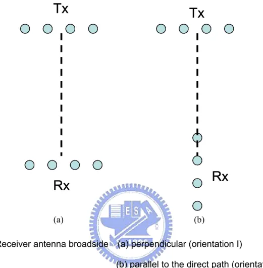
(28) In order to analyze how the local scatterer affects the UWB-MIMO capacity and correlation in the scenarios I, II, III and IV, we carry out the measurement in site D. The Room 202 and 203 are all enclosed with concrete walls and wooden doors. All of them are clustered with wooden chairs. During the measurement, we don’t move these chairs to stand for the environment with local scatterers (scenarios II/IV). And then we move these chairs far away Tx, Rx to stand for the environment without local scatterers (scenarios I/III). We adjust the element spacing of the virtual antenna arrays to investigate how the capacity varies is with different antenna spacing in the scenarios I, II, III and IV. At P1, P2, P3, P4, P5 and P6, both Tx and Rx antenna spacing is changed from 0.1 λ to 2.0 λ . In order to know the difference between LOS and NLOS condition, we measure at P1, P3 & P5 under the LOS condition, and P2, P4 & P6 under NLOS condition. In order to compare with the difference of varied antenna array orientation in the scenarios II, IV, V and VI, we do some measurement at site E and site F. For each transmit antenna position, the complex transfer functions were recorded for 10 receive antenna positions, 5 positions with the broadside of the virtual antenna perpendicular to the LOS (orientation I) and 5 positions with the broadside parallel to the LOS (orientation II). The array broadside orientation is shown in Fig. 3-5. The frequency response data have been exploited to analyze the UWB-MIMO channel characteristics. We observe the frequency response between 3.5GHz to 4.5GHz with 801 sweep points. Detailed measurement sites are shown in Table 5.. 15.

(29) Fig. 3-4 (a) Site A: 1st floor layout of the Microelectronics and Information System Research Center (MISRC). Fig. 3-4 (b) Site B: 2 nd floor layout of the MISRC. 16.

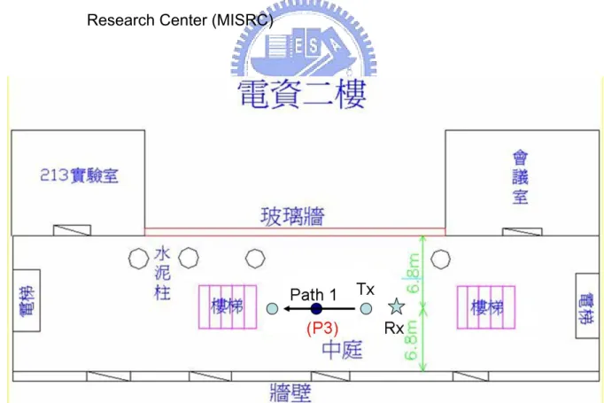
(30) Rx. v. Fig. 3-4 (c) Site C: Lab 213 layout of the MISRC. nd Fig. 3-4 (d) Site D: 2 floor layout of the 4th Engineering Building. 17.

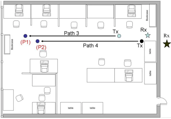
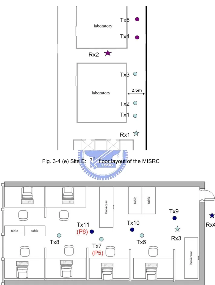
(31) th Fig. 3-4 (e) Site E: 7 floor layout of the MISRC. Fig. 3-4 (f) Site F: Lab 810 layout of the MISRC. 18.

(32) Tx. Tx. Rx. Rx (a). (b). Fig. 3-5 Receiver antenna broadside (a) perpendicular (orientation I) (b) parallel to the direct path (orientation II). 19.

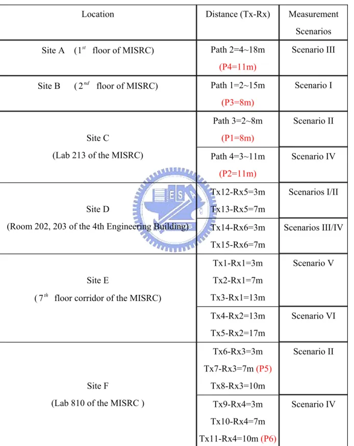
(33) Table 5 Measurement sites. Location. Distance (Tx-Rx). Measurement Scenarios. Site A ( 1st floor of MISRC). Path 2=4~18m. Scenario III. (P4=11m) Site B. ( 2 nd floor of MISRC). Path 1=2~15m. Scenario I. (P3=8m) Path 3=2~8m Site C. (P1=8m). (Lab 213 of the MISRC). Path 4=3~11m. Scenario II. Scenario IV. (P2=11m) Tx12-Rx5=3m Site D. Tx13-Rx5=7m. (Room 202, 203 of the 4th Engineering Building). Tx14-Rx6=3m. Scenarios I/II. Scenarios III/IV. Tx15-Rx6=7m Tx1-Rx1=3m Site E. Tx2-Rx1=7m. ( 7 th floor corridor of the MISRC). Tx3-Rx1=13m Tx4-Rx2=13m. Scenario V. Scenario VI. Tx5-Rx2=17m Tx6-Rx3=3m. Scenario II. Tx7-Rx3=7m (P5) Site F. Tx8-Rx3=10m. (Lab 810 of the MISRC ). Tx9-Rx4=3m Tx10-Rx4=7m Tx11-Rx4=10m (P6). 20. Scenario IV.

(34) Chapter 4 Propagation, Array Arrangement and Bandwidth on UWB-MIMO Capacity and Channel Correlations. To investigate the capacity and correlation properties of the UWB-MIMO channel under various propagation, array arrangement and bandwidth will be an interesting and important subject. In this chapter, the effects of propagation range, local scatterers, antenna spacing, array orientation and bandwidth on the UWB-MIMO capacity, EDOF and correlation are investigated through the measurement.. 4.1 UWB-MIMO capacity, EDOF and correlations evaluation From Eq. (2-2), the 4×4 MIMO capacity is given by Ci =. ⎛ ⎛ ρ 1 801 ⎞⎞ * log 2 ⎜⎜ det⎜ I 4 + H i ( f )H i ( f )⎟ ⎟⎟ ∑ 801 f =1 4 ⎠⎠ ⎝ ⎝ Hi ( f ) =. ^. ηk. Ti ( f ) ^. ηk N. 2. bits/s/Hz. n R nT f 1 = ∑∑∑ Ti, f , j ,k 4 × 4 × 801 f =1 j =1 k =1. 2. The capacity is calculated with ρ = 10dB and the measured 4×4 UWB-MIMO channel matrix, Ti (i is the time or snapshot index), which is realized through the measurement by Agilent 8719 ET vector network analyzer. The normalized UWB 21.

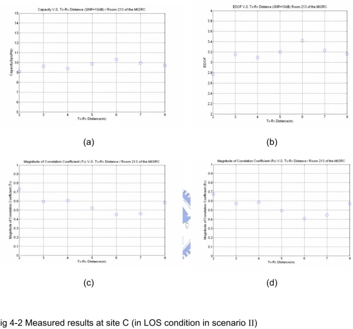
(35) ^. channel H i was calculated from (2-3) and (2-4), where η k. is the normalization factor. estimate. From Eq. (2-10), the EDOF is then obtained as EDOF =. min {nT , nR }. ∑ k =1. 1 1+. 4. λk ρ. And from Eq. (2-5) (2-6), the spatial correlation coefficient at Tx, Rx between elements are calculated.. 4.2 Propagation Range Effect (Scenarios I/II/III/IV) To investigate the propagation range effect on capacity, EDOF and correlations, we perform the measurement for a (4×4) UWB-MIMO system in two kinds of indoor environments: one in the lobby with light clutter (site A and site B) and another in the laboratory with heavy clutter (site C). We also consider the LOS and NLOS situation in two environments (scenarios I/II/III/IV). During the measurement, the antenna array broadside orientation direction is always perpendicular to the direct-path direction.. 4.2.1 LOS with light/heavy clutter (scenarios I/II) From Fig. 4-1 to fig. 4-2 illustrate the capacity, EDOF and correlations versus Tx-Rx distances in the LOS condition (scenarios I/II). By the chart of Fig. 4-1, we can find that in the scenario I, when Tx-Rx distance is in near distance, the capacity will be lower. But when distance is added to 10m, the capacity will not be changed obviously for distance increase. The reason is that because the Tx and Rx is very close, the correlations are relative higher at 1m, 2m and 3m (noted from Fig.4-1 (c) (d)). The LOS clutter strongly raises the correlation and then will cause the capacity reduced. In Fig. 4-1 (b) (EDOF vs. distance) can find the same tread as Fig. 4-1 (a). From fig. 4-2, we can find that capacity, EDOF and correlations are all similar for. 22.

(36) various distances in the scenario II. The reason is that there are heavy clutters in the laboratory so that when the Tx-Rx is in near distance, multipath will increase (compare with the scenario I), then correlations are not as high as the scenario II.. (a). (b). (c). (d). Fig 4-1 Measured results at site B (in LOS condition in scenario I) (a) Capacity versus distance; (b)EDOF versus distance; (c) ρ Tx versus distance;. (d) ρ Rx versus distance. 23.

(37) (a). (b). (c). (d). Fig 4-2 Measured results at site C (in LOS condition in scenario II) (a) Capacity versus distance;. (b) EDOF versus distance;. (c) ρ Tx versus distance;. (d) ρ Rx versus distance;. 24.

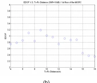
(38) 4.2.2 NLOS with light/heavy clutter (scenarios III/IV) Fig. 4-3, 4-4 illustrates the capacity, EDOF and correlations versus Tx-Rx distances in NLOS condition (scenarios III/IV). The main difference of Figs.4-1 (site B), 4-2 (site C) and Figs. 4-3 (site A), 4-4 (site C) is that there are many scatterers in the site C (compare with site A/B). By the chart of Fig. 4-3, we note that in the near distance, there is not a great effect on distance change to capacity, but when distance is during 16~18m, the capacity is low. We can find the reason out in the LAYOUT chart (Fig. 3-5(a)). As Tx-Rx distance is in 16~18m, Tx enter to a wide space and the multipath which RX received is reduced, so that the correlation coefficient is increase and then capacity decreased. The chart of Figs.4-3(c) (d) is the correlation coefficient for Tx, Rx and from the chart we can find that when Tx-Rx distance is in 16-18m, the correlation coefficient is higher. From fig. 4-4, we can find that capacity, EDOF and correlations are all similar for various distances in the scenario IV. The reason is same with situation II. Due to above results, we can conjecture that capacity is dependent of Tx-Rx distance in LOS with light clutter, i.e. capacity is lower when Tx-Rx distance in small AS (Angular Spread) of AOA/AOD. But capacity is independent of Tx-Rx distance in the environment with heavy clutter, i.e. capacity is similar for any Tx-Rx distance when AS of AOA/AOD is large. In addition, to compare Figs.4-1, 4-2, 4-3 and 4-4, we also can find that the capacity is higher under the environment that has scatterers around. With this phenomenon, we have a further discussion in the next section.. 25.

(39) (a). (b). (c). (d). Fig 4-3 Measured results at site A (in NLOS condition in scenario III) (a) Capacity versus distance; (b) EDOF versus distance; (c) ρ Tx versus distance;. (d) ρ Rx versus distance. 26.

(40) (a). (b). (c). (d). Fig 4-4 Measured results at site C (in NLOS condition in scenario IV) (a) Capacity versus distance;. (b) EDOF versus distance;. (c) ρ Tx versus distance;. (d) ρ Rx versus distance. 27.

(41) 4.3 Local Scatterer Effect (Scenarios I/II/III/IV) In this section, we analyze that how the local scatterer affects the UWB-MIMO capacity and correlation. In the first, we carry out the measurement in the classroom (site D) and consider the LOS and NLOS conditions (scenarios I/II/III/IV). During the measurement, the antenna broadside direction is perpendicular to the direct path direction. The antenna spacing has 0.25, 0.5, and 1 wavelength. Fig. 4-5 and fig. 4-6 show the capacity and correlations at two kinds of Tx-Rx distance under LOS condition (scenarios I/II). By the chart of fig.4-5(a), we can find that in the environment with local scatterers, the capacity is higher than the environment without local scatterers under any antenna spacing. And the same tread can be found as well in fig. 4-6(a). The reason is that the local scatterer reflect more multipath, and more multipath result in low correlation coefficient (noted from fig.4-5(b)(c), fig. 4-6(b)(c)) and then obtain higher capacity. The measured result under NLOS condition (scenarios III/IV) is showed in fig. 4-7 and fig. 4-8. We also find the similar outcome as the aforesaid conclusion. So we can conjecture that the environment with heavy clutter will have higher capacity than with light clutter in LOS and NLOS condition. Furthermore, capacity will be lower when antenna spacing is smaller than 0.5 wavelengths after compare above measured results. Because of this phenomenon, we take the further research in next section.. 28.

(42) (a). (b). (c) Fig. 4-5 Local Scatterers discussion under LOS condition in site D (scenarios I/II) (a) Capacity. (b) ρ Tx. (c) ρ Rx versus antenna spacing at Tx-Rx Distance=3m 29.

(43) (a). (b). (c) Fig. 4-6 Local Scatterers discussion under LOS condition in site D (scenarios I/II) (a) Capacity. (b) ρ Tx. (c) ρ Rx versus antenna spacing at Tx-Rx Distance=7m 30.

(44) (a). (b). (c) Fig. 4-7 Local Scatterers discussion under NLOS condition in site D (scenarios III/IV) (a) Capacity. (b) ρ Tx. (c) ρ Rx versus antenna spacing at Tx-Rx Distance=3m 31.

(45) (a). (b). (c) Fig. 4-8 Local Scatterers discussion under NLOS condition in site D (scenarios III/IV) (a) Capacity. (b) ρ Tx. (c) ρ Rx versus antenna spacing at Tx-Rx Distance=7m 32.

(46) 4.4 Antenna Spacing Effect (Scenarios I/II/III/IV) In the UWB-MIMO system, channel capacity may be improved by adaptively changing the element spacing. Changing the element spacing is a way to provide spatial diversity to a MIMO link without increasing the number of antenna array elements [17]. In this section, we adjust the element spacing of virtual antenna arrays to investigate how the capacity varies is with small changes in element locations. During the measurement, the measurement points from P1 to P6 have been selected to consider scenarios I/II/III/IV. And the antenna broadside direction is perpendicular to the direct path direction. Fig. 4-9(a) (b) (c) illustrates the capacity, Tx and Rx correlation coefficients versus antenna spacing for LOS condition respectively (scenarios I/II). For comparison, the capacity for a perfect Rayleigh channel is plotted. To this end, 10 6 random matrices with independent, identically distributed complex numbers (normal distribution with zero mean and variance σ = 1 ) were generated and the averaged capacity was calculated. In the LOS condition, the capacity is low to 6.5 bps/Hz at 0.1λ spacing and dramatically rises to about 10 bps/Hz at 0.5λ spacing. Afterward, capacity grows slowly with the antenna spacing increasing. Both ρ Tx and ρ Rx decrease with antenna spacing increasing. Fig. 4-10(a) (b) (c) illustrates the capacity, Tx and Rx correlation coefficients versus antenna spacing for NLOS condition respectively (scenarios III/IV). In the NLOS condition, the capacity is low to about 7 bps/Hz at 0.1λ spacing and rise to about 10.5 bps/Hz at 0.5λ spacing. The capacity is not changed while antenna spacing is larger than 1λ. From the result of this section, we can see that antenna spacing may affect UWB-MIMO capacity significantly under any environment (scenarios I/II/III/IV). And we can find that the capacity increases as the element spacing increases and it saturates when the spacing is larger than 0.5 λ . This reveals that the correlation distance between the elements in indoor environments is about 0.5 λ . 33.

(47) (a). (b). (c) Fig. 4-9. (a) Capacity (b) ρ Tx (c) ρ Rx versus antenna spacing in LOS condition (P3 belong to the scenario I and P1、P5 belong to the scenario II) 34.

(48) (a). (b). (c) Fig. 4-10. (a) Capacity (b) ρ Tx (c) ρ Rx versus antenna spacing in NLOS condition (P4 belong to the scenario III and P2, P6 belong to the scenario IV). 35.

(49) 4.5 Array Orientation Effect To investigate the array orientation effect on capacity and correlation, we perform the measurement for a (5×5) UWB-MIMO system in two kinds of indoor environments: one is in a corridor(site E, scenarios V/VI), another one is in a laboratory(site F, scenarios II/IV). During the measurement, two kinds of array orientation are considered: the antenna array broadside orientation direction is perpendicular (orientation I) and parallel (orientation II) to the direct-path direction [4] [18].. 4.5.1 Measured results in the scenarios V and VI (corridor, site E) In Fig. 4-11 and 4-12 (site E), the mean capacities for different array size ( nT = n R ) is shown. From Fig. 4-11, we observe a significant different between the capacities achieved by parallel and perpendicular arrays in all distance. The perpendicular array results in a higher capacity gain than the parallel array in LOS condition (scenario V). This is because the perpendicular receiver array allows additional spatial dimensions of the UWB-MIMO channel by distinguishing between those scatterers on the opposite walls of the corridor with the same distance to the receiver array. The parallel array would be unable to distinguish between these ‘mirrored’ scatterers and hence capacity gain for orientation II is significantly lower. Fig. 4-13 shows the correlation coefficients for scenario V. As expected, the receiver correlation is higher when the broadside of the receive array is parallel to LOS in all distance because perpendicular array will distinguish more multipath, so can reduce the correlation coefficient. The transmit correlations are almost equal for two orientations. The above effect is that we measured for LOS condition in the corridor (scenario V). And now let us observe that in case of NLOS condition (scenario VI), whether the characteristic we measure is the same as LOS condition? Fig. 4-12 is the result of measured in the scenario VI. From fig.4-12, we find that orientation I results in a higher capacity gain 36.

(50) than orientation II. The reason is the same as above result. Fig. 4-14 shows the correlation coefficient for the scenario VI. In addition, we also observe the capacity increases linearly with the number of antenna elements, indicating that there are a sufficient number of strong MPCs providing independent transmission paths for different data streams.. (a). (b). 37.

(51) (c) Figure 4-11 Capacity versus array orientations in the scenario V (site E, LOS) (a) Tx-Rx Distance=3m (b) Tx-Rx Distance=7m (c) Tx-Rx Distance=13m. (a). (b) Figure 4-12 Capacity versus array orientations in the scenario VI (site E, NLOS) (a) Tx-Rx Distance=13m. (b) Tx-Rx Distance=17m 38.

(52) (a). (d). (b). (e). (c). (f). Fig 4-13 ρ Tx and ρ Rx versus array orientations in the scenario V (site E, LOS) (a) ρ Tx Tx-Rx Distance=3m. (d) ρ Rx Tx-Rx Distance=3m. (b) ρ Tx Tx-Rx Distance=7m. (e) ρ Rx Tx-Rx Distance=7m. (c) ρ Tx Tx-Rx Distance=13m. (f) ρ Rx Tx-Rx Distance=13m. 39.

(53) (a). (c). (b). (d). Fig 4-14 ρ Tx and ρ Rx versus array orientations in the scenario VI (site E, NLOS) (a) ρ Tx Tx-Rx Distance=13m. (c) ρ Rx Tx-Rx Distance=13m. (b) ρ Tx Tx-Rx Distance=17m. (d) ρ Rx Tx-Rx Distance=17m. 40.

(54) 4.5.2 Measured results in the scenarios II and IV (laboratory, site F) Above-mentioned is the measured result in the corridor (scenarios V/VI), and then we observe the result in the laboratory (scenarios II/IV) below. Fig. 4-15 and 4-16 illustrate the capacity for both LOS and NLOS conditions in the laboratory (scenarios II and IV). From Fig. 4-15, in the far distance between Tx, Rx the capacity for orientation I is more than orientation II, but when the near distance between Tx, Rx, it is similar for both orientation. The reason for this phenomenon is that when the distance between Tx, Rx is far, the correlation coefficient will be drop. Therefore, when receiver array broadside parallel to the direct path will cause correlation coefficient increased, then capacity will be drop. But when the distance between Tx, Rx is near, the path of LOS is stronger than others. So both two orientations have high correlation coefficient, and then capacity is low equally. Fig. 4-17 shows the correlation coefficient in the scenario II. From Fig.4-16 we can see that in the NLOS condition, the capacity is similar for both orientations in all distance between Tx and Rx. This is because no dominant path exists under NLOS scenarios where no additional spatial diversity can be obtained by changing the orientations. Fig. 4-18 shows the correlation coefficient in the scenario IV.. (a) 41.

(55) (b). (c). Figure 4-15 Capacity versus array orientations in the scenario II (site F, LOS) (a) Tx-Rx Distance=3m (b) Tx-Rx Distance=7m (c) Tx-Rx Distance=10m. 42.

(56) (a). (b). (c) Figure 4-16 Capacity versus array orientations in the scenario IV (site F, NLOS) (a) Tx-Rx Distance=3m. (b) Tx-Rx Distance=7m 43. (c) Tx-Rx Distance=10m.

(57) (a). (d). (b). (e). (c). (f). Fig 4-17 ρ Tx and ρ Rx versus array orientations in the scenario II (site F, LOS) (a) ρ Tx Tx-Rx Distance=3m. (d) ρ Rx Tx-Rx Distance=3m. (b) ρ Tx Tx-Rx Distance=7m. (e) ρ Rx Tx-Rx Distance=7m. (c) ρ Tx Tx-Rx Distance=10m. (f) ρ Rx Tx-Rx Distance=10m. 44.

(58) (a). (d). (b). (e). (c). (f). Fig 4-18 ρ Tx and ρ Rx versus array orientations in the scenario IV (site F, NLOS) (a) ρ Tx Tx-Rx Distance=3m. (d) ρ Rx Tx-Rx Distance=3m. (b) ρ Tx Tx-Rx Distance=7m. (e) ρ Rx Tx-Rx Distance=7m. (c) ρ Tx Tx-Rx Distance=10m. (f) ρ Rx Tx-Rx Distance=10m 45.

(59) 4.6 Capacity Loss In this section, for a more in-depth analysis of the performance of UWB-MIMO systems at locations with high SNR and high antenna correlation, measurements were done to investigate the effects of SNR and antenna correlation on UWB-MIMO channel capacity. First of all, we define capacity loss ( C loss ) as. C loss = 1 −. C measure ( SNR) Ci.i.d ( SNR). (4-1). The capacity loss for different measurement is calculated for comparing the measured capacity and the optimum case at the same SNR.. 4.6.1 Capacity Loss for different antenna spacing The measurement points from P1, P2 have been selected to consider LOS and NLOS condition. The channel capacity loss with respect to the received SNR for various antenna spacing are calculated from Eq.4-1 and shown in Fig.4-19. From Fig.4-19, we can see that for small antenna spacing, when SNR increases, the channel capacity loss increases initially but decreases gradually afterwards. The reason for this is that when SNR is low, a comparison of the ideal channel and the measured channel shows that there is a channel capacity gap which widens as SNR increases. However, when SNR increases beyond a certain value, this gap becomes constant and independent of the SNR. It means that the relative channel capacity loss due to the effect of high antenna correlation is reduced as SNR increases. In other words, Fig.4-19 shows that in small antenna spacing, the UWB-MIMO system is robust against the high antenna correlation when SNR is high.. 46.

(60) (a). (b) Fig. 4-19 Capacity loss versus SNR at different antenna spacing (a) measured point P1 in LOS condition (b) measured point P2 in NLOS condition 47.

(61) 4.6.2 Capacity loss for different Tx-Rx distance in LOS condition From section 4-2, we know that when Tx-Rx distance is in near distance, channel capacity is low and antenna correlation is high in the LOS condition. However from the propagation point of view, the dominant LOS signal component would also lead to a high receive signal power which increases channel capacity when Tx-Rx distance is in near distance. It becomes a situation where there is a tradeoff between the effects of increased correlation and increased receive SNR on the UWB-MIMO channel capacity. Therefore we make a further analysis in the site B and site C. Fig.4-20 illustrates the capacity loss versus SNR at different Tx-Rx distance in the scenarios I and II. From Fig.4-20 (a), we can see that for small Tx-Rx distance, when SNR increases, the channel capacity loss increases initially but decreases gradually afterwards. The reason is same as section 4.6.1. But when Tx-Rx distance is added to 10m, the capacity loss is almost same at different SNR. This phenomenon tell us that when Tx-Rx distance is in near distance, although antenna correlation is high but if received SNR is excess 10dB then the UWB-MIMO system is robust against the antenna correlation. Above results are measured in the scenario I, now we observe the measured result in the scenario II. The main difference of scenarios I and II is that there are heavy clutter in the scenario II. From Fig.4-20 (b), we can see that when Tx-Rx distance is in near distance, the capacity loss is not as high as measured results in the scenario II. This is because there are scatterers in the scenario II, so antenna correlation is not as high as the scenario I. So if antenna correlation is not high, capacity loss will not change when SNR increases. From above results, we find that the loss of channel capacity owing to high correlation is significantly reduced when the SNR is sufficiently high. 48.

(62) (a). (b) Fig. 4-20 Capacity loss versus SNR at different Tx-Rx distance in LOS condition (a) measured path1 in the scenario I (site B) (b) measured path3 in the scenario II (site C) 49.

(63) 4.7 Bandwidth Effect In this section, we investigate the impact of the signal bandwidth on the UWB-MIMO capacity. We choose 20、40、80、500 and 1000M signal bandwidths to see how it affects the capacity. From figures 4-21 we can see that a small difference in capacity when using the larger bandwidth. Hence not much frequency diversity is available.. (a). (b) Fig. 4-21 CDF for capacity (a) LOS (b) NLOS 50.

(64) Chapter 5 Characterization of UWB Channels for indoor environment. This chapter presents the characterization of UWB channels for indoor environment with above measured data. This channel characterization addresses only the small scale propagation properties. The Saleh-Valenzuela (S-V) model [19] is used as a basis for our UWB channel model.. 5.1 Radio Channel Model For the small scale properties, we have chosen the S-V model [19] as a basis for parameter extraction. In the S-V model, multipath components (MPCs) behave like rays arriving in clusters. This results in the following discrete time impulse response for the channel: L. K. h(t ) = Σ Σ β k ,l δ (t − Tl − τ k ,l ) l =0 k =0. (5-1). where β k ,l is the tap weight of the kth component in the lth cluster, Tl represents the arrival time of the lth cluster, and τk,l is the arrival time of the kth arrival within the lth cluster, relative to Tl. K is the total number of MPCs in a cluster and L is the total number of clusters. By definition, τ o ,l = 0 .. The distributions of the cluster and ray arrival times, i.e. Tl and τk,l , are given by Poisson processes in the following equations: 51.

(65) p (Tl Tl −1 ) = Λ exp ⎡⎣ −Λ (Tl − Tl −1 ) ⎤⎦ ,. (. ). (. l >0. ). p τ k ,l τ ( k −1),l = λ exp ⎡⎣ −λ τ k ,l − τ ( k −1),l ⎤⎦ ,. k >0. (5-2). where Λ is the cluster arrival rate and λ is the ray arrival rate.. βkl is a Rayleigh-distributed random variable with a mean-square value that obeys a double exponential decay law, according to. β 2 kl = β 2 ( 0,0 ) exp ( −Tl / Γ ) exp ( −τ kl / λ ) ,. (5-3). where β 2 ( 0,0 ) is the average power of the first arrival of the first cluster. This average power is a function of the distance separating the transmitter and receiver. Fig. 5-1 illustrates this, showing the mean envelope of a three-cluster channel. Hence, in order to characterize the multipath statistics of the channel, the parameterΓ,. γ, Λ, λ (i.e. cluster and ray power-decay time constants and arrival rates) have to be extracted.. Figure 5-1 An illustration of exponential decay of mean cluster power and ray power within clusters.. 52.

(66) 5.2 Model Parameters from the Data The VNA measurements yield the complex frequency responses of the channel. The time domain impulse responses are obtained from these frequency domain data by using simple IFFT. The above procedure yields the PDP for each channel impulse response. The number of clusters and their respective arrival times, w.r.t. To are obtained from manual inspection of each PDP.. 5.2.1 Cluster and Ray Power-Decay Time Constants, Γ and γ For the extraction of Γ, the power level of the MPCs in each cluster is divided by. β 2 ( 0,0 ) . Then, all the cluster arrivals, i.e. first MPC in each cluster β0,l are superimposed and plotted on a semi-log graph against Tl . Γ is obtained from the plot by applying a least square curve fitting program. For the extraction of γ , it is assumed in this paper that the MPCs in all clusters decay at a constant rate. The MPCs in each cluster is first normalized w.r.t. the power of the first MPC in that cluster. All the clusters from all PDPs are then superimposed and plotted on a semi-log graph against τk,l.. 5.2.2 Cluster and Ray Arrival Rates, Λ and λ Cluster and ray arrivals are described by the Poisson process in (5-2). For cluster arrivals, T0 is set to zero, with all other Tl adjusted accordingly. For ray arrivals, τ0,l is set to zero, with all other arrival times of rays in the same cluster adjusted accordingly. With these adjustments, the empirical CDF is obtained from the measured data and least mean square (LMS) criteria is used to fit the best exponential CDF (CDF of a Poisson process is an exponential function) to the empirical CDF.. 53.

(67) 5.3 Measured results in the Scenarios I, II, III, and IV Fig 5-2, 5-3, 5-4, 5-5 show four parameter of S-V model for scenarios I, II, III and IV.. Tl. τk,l (a). (b). Tl – Tl-1. τk,l-τk-1,l. (c). (d). Fig 5-2 Four parameters of S-V model for scenario I (a) Cluster decay exponent fit for scenario I ( Γ = 30.47 ns ) (b) Ray decay exponent fit for scenario I. ( γ = 27.12 ns ). (c) Cluster arrival rate fit for scenario I. (1. (d) Ray arrival rate fit for scenario I. ( 1 = 4.47 ns ). Λ. λ. 54. = 23.7 ns ).

(68) Tl. τk,l. (a). (b). Tl – Tl-1. τk,l-τk-1,l. (c). (d). Fig 5-3 Four parameters of S-V model for scenario II (a) Cluster decay exponent fit for scenario II ( Γ = 27.75 ns ) (b) Ray decay exponent fit for scenario II. ( γ = 30.77 ns ). (c) Cluster arrival rate fit for scenario II. (1. Λ. = 20.51 ns ). ( 1 = 3.35 ns ). (d) Ray arrival rate fit for scenario II. λ. 55.

(69) Tl. τk,l (a). (b). τk,l-τk-1,l. Tl – Tl-1 (c). (d). Fig 5-4 Four parameters of S-V model for scenario III (a) Cluster decay exponent fit for scenario III ( Γ = 43.68 ns ) (b) Ray decay exponent fit for scenario III. ( γ = 40.37 ns ). (c) Cluster arrival rate fit for scenario III. (1. (d) Ray arrival rate fit for scenario III. ( 1 = 2.39 ns ). Λ. λ. 56. = 22.91 ns ).

(70) Tl. τk,l. (a). (b). τk,l-τk-1,l. Tl – Tl-1 (c). (d). Fig 5-5 Four parameters of S-V model for scenario IV (a) Cluster decay exponent fit for scenario IV ( Γ = 41.84 ns ) (b) Ray decay exponent fit for scenario IV. ( γ = 41.1 ns ). (c) Cluster arrival rate fit for scenario IV. (1. (d) Ray arrival rate fit for scenario IV. ( 1 = 1.98 ns ). Λ. λ. 57. = 25.2 ns ).

(71) Table 6 Summary of four parameters of S-V model for scenarios I, II, III and IV LOS with light NLOS with light LOS with heavy NLOS with heavy clutter. clutter. clutter. clutter. 6.38. 7.52. 7.17. 8.59. Γ. 30.47 ns. 43.68 ns. 27.75 ns. 41.84 ns. std. 6.06. 16.92. 4.21. 16.37. γ. 27.12 ns. 40.37 ns. 30.77 ns. 41.1 ns. std. 9.73. 21.06. 10.66. 18.04. 1/Λ. 23.7 ns. 22.91 ns. 20.51 ns. 25.2 ns. 1/λ. 4.47 ns. 2.39 ns. 3.35 ns. 1.98 ns. Mean No. of clusters. 5.4 Analysis of Measured results Table 6 is a summary of four parameters of S-V model for scenarios I, II, III and IV. From Comparing scenasios I and III, we can see that Γ decay faster in the LOS condition than in the NLOS condition. This is because that in the LOS condition, direct path is stronger than others. The same tread is find between scenario II and IV. From [19] we can see that in the broadbasnd system, Γ、 γ have different decay slope, but we find that in the UWB system Γ、 γ have similar decay slope from our measured results.. 58.

(72) Chapter 6 Hybrid UWB MIMO Channel Model In this chapter, we propose a set of channel models applicable to indoor UWB-MIMO systems. The newly developed UWB MIMO channel models are based on 802.11n channel model [12] to modify and combing UWB channel model. A step-wise development of the new models follows: In each of the four models (A-D) distinct clusters were identified first. The number of clusters varies from 6 to 9, depending on the model. The power of each tap in a particular cluster was determined by using the parameter of above UWB channel model (chapter 5). Next, angular spread (AS), angle-of-arrival (AOA) and angle of departure (AOD) values were assigned to each tap and cluster (using statistical methods) that agrees with experimentally determined values reported in the literature. Cluster AS was experimentally found to be in the 20o to 40o range [10, 11, 22-25] and the mean AOA was found to be random with a uniform distribution. With the knowledge of each tap power, AS, and AOA (AOD), for a given antenna configuration, the channel matrix H can be determined. The channel matrix H fully describes the propagation channel between all transmit and receive antennas. If the number of receive antennas is n and transmit antennas is m, the channel matrix H has a dimension of n x m. To arrive at channel matrix H, we use a method that employs correlation matrix and i.i.d. matrix (zero-mean unit variance independent complex Gaussian random variables). The correlation matrix for each tap is based on the power. 59.