治癒模式之半母數迴歸分析

國立交通大學

統計學研究所

博 士 論 文

治癒模式之半母數迴歸分析

Semiparametric Regression Analysis

in Presence of Non-susceptibilit

y

研究生： 許秋婷

指導教授： 王維菁 教授

治癒模式之半母數迴歸分析

Semi-parametric Regression Analysis

in Presence of Non-susceptibility

研 究 生：許秋婷 Student：Chew-Teng

Kor

指導教授：王維菁 教授 Advisor：Weijing Wang

國 立 交 通 大 學

統 計 學 研 究 所

博 士 論 文

A Dissertation

Submitted to Institute of Statistics College of Science

National Chiao Tung University in partial Fulfillment of the Requirements

for the Degree of Doctor of Philosophy

in Statistics

Institute of Statistics, National Chiao Tung University Hsinchu, Taiwan, R.O.C.

治癒模式之半母數迴歸分析

學生：許秋婷 指導教授：王維菁

國立交通大學統計學研究所 博士班

摘 要

本論文針對存活資料，考慮“不受感染體質＂(nonsusceptibility)者之存在， 在混合模式架構下提出半母數迴歸分析方法。我們採用邏輯斯模式分析解釋變數與 “發病與否＂的關係。針對受感染體質者之“潛在發病時間＂，我們探討兩類迴歸 模式之推論問題。第一類模式包含常見的加速失敗模式和位移模式，我們利用計數 程序之機率性質以建構估計函數，並進一步提出模式選取方法。第二類為線性轉換 模式，包含等比風險模式與等比勝負比模式。我們採用概似函數法做為參數估計的 原則，除了分析獨立設限的情況外，並進一步提出當存在競爭風險時，如何修正模 式假設與推論方法。兩個研究方向都利用 EM 的技巧，以補插法處理感染體質不確 定之觀測值。我們透過模擬實驗評估所提出方法在有限樣本下之表現。 關鍵字: 混合模式，不受感染體質，補插法，半母數線性迴歸，線性轉換模式， 鞅估計函數，對數秩統計量，競爭風險。

Semi-parametric Regression Analysis in Presence of

Non-susceptibility

Student: ChewTeng Kor Advisor:Weijing Wang

Institute of Statistics

National Chiao Tung University

Abstract

In this thesis, we consider semiparametric regression analysis for survival data in presence of non-susceptibility or cure. The mixture framework is adopted in analysis of such data. The incidence rate is assumed to follow the logistic regression model and the latency distribution is studied under two types of semiparametric regression models. One class refers to the semi-parametric linear regression model which includes the AFT and location-shift models as special cases. We propose estimating functions and also a model checking procedure based on properties of counting processes. The other class is known as transformation models which contain the proportional hazards model and proportional odds model. The likelihood principle is adopted for parameter estimation. We examine two situations of independent and dependent censoring respectively. In both research directions, the principle of EM is applied to handle uncertain susceptibility status. Simulation results are provided to examine the finite-sample properties of the proposed methods.

Keywords: Competing risk; EM, Logistic regression; Linear regression model; Latency distribution; Log-rank statistic; Transformation model; Martingale; Mixture model; Non-susceptibiblity.

誌 謝

人生的機遇總是很奇妙，如同蝴蝶效應般的影響著往後的人生規劃。或許 很多決定是不假思索順勢而為，感謝上帝的眷顧，讓我擁有這段美麗的研究 生生活。博士畢業也代表我在台灣 12 年學生旅程的 ending，接下來我將轉 換身份繼續出發，期許自己能有更好的表現答謝支持鼓勵我的師長，家人和 朋友們。 首先，我要感謝我的指導教授王維菁教授。我自覺自己是個迷糊，缺乏組織 能力的學生。在這方面，王老師時而充滿著母愛般耐心的提醒我，時而如嚴 父般地教誨改進我缺點，我內心充滿感激老師的用心良苦。回想當初在我研 究遇到瓶頸，心情沮喪挫折之時，王老師比任何人更擔憂我的前途，也與我 討論了許多改進的方向。我由衷的感謝老師的教育。 我還要感謝洪慧念教授的輔助指導，當我在理論證明或是模擬程式有困難的 時候，洪老師總是不厭其煩的指導我，並指示出可能出錯的問題。我也很感 謝洪老師分享生活上經驗予我參考。 另外，我也要感謝我的口試委員 鄭光甫教授，陳珍信教授和程毅豪教授特地 在來新竹幫我口試。老師們撥空對我論文的架構提出寶貴的意見，使我的博 士論文更為完善。當中老師們也提供了許多論文題目予我分享，對後續研究 方向的確立幫助甚大。我將繼續保持謙卑，不倦的學習態度面對往後的研究 工作，再次感謝老師們的指導與教育。 在交大八年的研究生生涯中，我也要感謝統計所所有的老師的教育。感謝所 辦郭姐身兼諮商老師輔導我在家庭相處，婚姻感情的處理態度，我懷念跟郭 姐一起午休散步的日子。感謝研究室的伙伴們和一起在課業打拼的同學們， 我很高興有你們的陪伴。因為有你們的陪伴學習，使我在交大有美好的學習 回憶。 在此，我要特別的感謝我先生新淵永遠支持我任何的決定。當我學習上遇到 挫折沮喪時常常鼓勵我，並安慰我說“蹲下是為了跳更高＂。當我在煩惱畢 業問題時，總是安慰我說“不急慢慢來，讓我照顧你＂。因為有你的陪伴， 給了我重新出發勇氣。最後也要感謝我親愛的家人們，因為有你們的栽培， 才能成就今天的我。 最後，僅將此論文獻給敬愛的家人，老師，同學和關心我的人，與我一同分 享此論文的喜悅與榮耀。 許秋婷 謹誌於 國立交通大學統計所 中華民國九十九年六月

Table of Contents

1 Introduction

1

1.1 Literature background

1

1.2 Outline

of

the

thesis

2

2 Literature Review for Semi-parametric Linear Models with Cure 4

2.1 Overview

4.

2.2 M-Estimation by Li & Taylor (2002)

7

2.3 Log-rank type Estimation by Zhang & Peng (2007)

8

2.4 Sketch of Numerical Algorithm for EM-type Estimation

9

3 Proposed Approach for Semiparametric Linear Models

11

3.1 Martingale estimating function based on complete data

11

3.2 The proposed estimating functions

12

3.3 Large

sample

analysis

13

3.4 Numerical algorithm and variance estimation

17

3.4.1 Re-sampling based on bootstrap approach

18

3.4.2 Re-sampling based on pivotal estimating function

18

3.5 Model

Checking

20

3.6 Simulation

analysis

22

3.6.1 Data generation 22

3.6.2 Simulation results 22

4 Literature Review for Transformation Models with Cure

25

4.1 Background

26

4.3 Likelihood approach under the

PH

model

26

4.4 Moment approach for the class of transformation models

29

5 Proposed Approach for Transformation Cure Model under

Independent

Censoring 32

5.1 Model

assumptions

32

5.2 Likelihood analysis for complete data

33

5.3 Imputation for handling missing data

36

5.4 Numerical

algorithms

37

5.5 Simulation

analysis

37

5.5.1 Data generation 37

5.5.2 Simulation results 38

6 Proposed Approach for Transformation Cure Model Under

Dependent

Censoring

40

6.1 Model

assumptions

40

6.2 Imputation

under

the

new

models

41

6.3 Likelihood analysis under dependent censorship

42

6.4 Score equations under dependent censorship

45

6.5 Numerical

algorithm 49

6.6 Simulation

analysis

50

6.6.1 Data generation 50 6.6.2 Simulation results 52

Conclusion

53

References

54

Appendix 56

Chapter 1

Introduction

1.1 Literature background

Traditional survival models assume that every subject in the study will eventually experience the event of interest. However, Kaplan-Meier curves based on empirical data often level off at the right tail and exhibit a stable plateau. Survival analysis which accounts for the possibility of cure or non-susceptibility has received increasing attentions in the literature since it provides reasonable explanations for some scientific phenomenon. The most popular approach to analyzing survival data in presence of cure is to represent the population as a mixture of susceptible and cured subjects. Define  as the indicator of susceptibility. The population is divided into two groups: the susceptible with   and the cure with 1   . For 0  1, define T as the time to the failure event. When   , T is undefined or conventionally set to be infinity. Accordingly one 0 can write

Pr(T t ) Pr(T t | 1) Pr(  1) Pr(  . 0)

In presence of covariates denoted by Z , the mixture model can be written as

Pr(T t Z | )Pr(T t | 1, ) Pr(Z  1| )Z Pr( 0 | )Z . (1.1)

Under the above mixture framework, most literature assumes that the incidence function follows the logistic regression model which can be written as

0 Pr( 1| )Z  ( | )Z 0 0 exp( ) 1 exp( ) T T Z Z     . (1.2)

Different proposals for modeling the latency variable T|  have appeared in the literature. 1 Parametric models including the Weibull, generalized Gamma and generzlized F have been proposed by Farewell (1982), Yamaguchi (1992) and Peng et al. (1998) respectively. Semi-parametric models are more popular choices due to their flexibility and robustness. Most popular semi-parametric models, after some transformation, can be written as a linear regression form. For modeling T|  , one can write 1

0 ( ) T

h T Z   , (1.3)

where ₀:p is the unknown regression parameter of interest, ( )1 h  is a monotone functions and  is the error term whose distribution does not depend on Z .

Now we discuss two general classes of model (1.3). One type of models, which refers to semi-parametric linear models, assumes that ( )h  is given but the error distribution is unknown. For example if ( )h t log( )t , the model becomes an accelerated failure time model. If ( )h t  , it t comes a location-shift model. Hence unknown parameters become ₀ and 0

( ) Pr( )

F t_    . The t

other class, known as transformation models, assumes that h( ) is unknown but the distribution of  is specified. For the Cox proportional hazards (PH) model,  follows the extreme value

distribution with 0

( ) exp{ exp( )}

S t_   t and 0

( )t exp( )t



  . For the proportional odds model, 

follows the logistic distribution with 0

( ) exp( ) /{1 exp( )}

S t_  t  t . Unknown parameters contain

0

 and h( ) .

Nonparametric analysis for cure models with right censored observations may suffer from the inherent non-identifiability problem. A censored observation indicates two possible situations: the subject may be susceptible but the event has not occurred by the end of study; or he/she is cured. To distinguish the two different cases, the follow-up period has to be long enough to observe the susceptible ones as much as possible. The book of Maller and Zhou (1996) discusses the issue of identifiability and presents nonparametric tests to verify the condition of sufficient follow-up. Despite the theoretical contribution, these tests are not practical due to their low power. Therefore for practical applications, expert opinions about whether cure exists or not are important for choosing an appropriate model (Farewell, 1986).

1.2 Outline of the thesis

This thesis considers semi-parametric inference based on models in (1.2) and (1.3). The problem of non-identifiability is not as serious as in the nonparametric setting since additional

model assumptions will be imposed. For the latency distribution, we consider both classes of models. We review the literature for semi-parametric linear models and present our proposal in Chapter 2 and 3 respectively. Then we consider transformation models in Chapters 4, 5 and 6. Chapter 4 reviews existing literature and Chapters 5 and 6 present our proposals under independent censoring and dependent censoring respectively. Chapter 7 contains concluding remarks.

Chapter 2

Literature Review for

Semi-parametric Linear Models with Cure

2.1 Overview

Under the mixture framework, assume that

0 Pr(_i 1|Z_i) _i( | )Z 0 0 exp( ) 1 exp( ) T i T i Z Z     and for _i  , we have 1

0 ( )_{i i}T _i

h T Z   ,

where h( ) is specified and ( 1,..., )_i i n form an iid sample with an unknown marginal distribution independent of Z . Define _i f t_0( ) , F t_0( ) , S t_0( ) and 0_( )t as the density, distribution, survival and cumulative hazard functions of  respectively, all of which are unspecified. In this chapter, we review existing literature for estimating ( ₀, ₀) in presence of the nuisance function S t_0( ). Note that when ( )h t log( )t , the model becomes the AFT model; and if h t( ) , the model becomes the location-shift model. t

Let C be the censoring variable for the ith subject. We will assume that _i C and _i T are _i

independent. Denote observed data as



(X_i, ,_i Z_i), 1,...,i n



, where X_i  T_i C_i and

( )

i I Ti Ci

   . Before we discuss specific methods, it is useful to examine the inference problem using the classical likelihood approach. One can express the data under the scale of the error variable. Let _i()h

 

T_i Z_iT , _iC()h

 

C_i Z_iT and  _i( )h X( _i)Z_iT. Note that

0 ( )

i

  has the same distribution as  when ₀ is the true value of . The likelihood function can be written as 0 ( , , ) L   f





( 1) 0 1 ( ) ( ) i n _I i i i f_          



_  _ 0





( 0) ( ) ( ) (1 ( )) I i i S i i            _    _ , (2.1a)

where ( ) _i exp(Z_iT) /{1 exp( Z_iT)}.

logarithm.

The idea of EM algorithm is often adopted in statistical inference of cure models. If “complete” data denoted as



(X Z_i, _i, , _{i i}), 1,...,i n



are available, the above likelihood in (2.1a) can be simplified as:











₀ ( 1) ₀ ( 0, 1) 1 ( ) ( ) i ( ) ( ) i i n _{I I} i i i i i f_  S_                      



 





( 0, 0)



1 _i( ) I i i . (2.1b) The resulting log-likelihood function can be written as:

log ( , ,L   f_0) ( , ,  f_0)₁( ) ₂( , f_0) where 1( )   1 log ( ) n i i i     



1 (1 ) log{1 ( )} n i i i       



; (2.3a) 0 2( , f )  0





1 log ( ) n i i i f_     



 0





1 (1 ) log ( ) n i i i i S_       



 . (2.3b)

Notice that the parameters  and  become separated in (2.3a) and (2.3b) respectively. Accordingly the score functions for  and  become

1( ) /     1 ( ) ( ) n i i i i       



 1 { ( )} (1 ) 1 ( ) n i i i i          



 , (2.4a) 0 2( , f ) /     0 0 0 0 1 ( ( )) ( ( )) (1 ) ( ( )) ( ( )) n i i i i i i i i i f f Z f S                         



 _{ } , (2.4b) where f t( ) f t( ) /t and ( )    ( ) /. The above derivations imply that  and  can

be estimated separately if the value of _i could be observed for all i1,...,n and 0 ( )

f t_ , or at

least its parametric form, is known. However these two conditions often do not hold in practical applications. Now we discuss how to handle these problems.

To deal with possibly unknown value of _i, a common approach is to replace it by an imputed value, often an estimate of its conditional mean given observed data. Notice that when

1

i

  , 1_i  ; but when _i  , 0 _i is unknown. It follows that ) , | ( ) , , | ( _i X_{i i} Z_{i i} E _i T_i C_i X_i Z_i E        .

Under the imposed models, we write 0 0 0 ( _i| _i, ,_{i i}) _i (1 _i) _i( , , ) E  X  Z     w   S_ , (2.5) where ( , , ) i w   S_ ( ) ( ( )) ( ) ( ( )) {1 ( )} i i i i i S S                    . (2.6)

In estimation, the weight w_i( , ,  S_) is often treated as a fixed value by plugging in previous estimates of 0

0 0

( ,  ,S_). This technique is commonly seen for analyzing missing data.

Under the semi-parametric setting, the major challenge is the log-likelihood function in (2.3b) or the score equation in (2.4b) which involves the nuisance functions f_0(.), f_0(.) and S_0(.), the first two of which are complicated. Existing methods try to get rid of the density function

0 (.)

f_ in the estimation but still keep the survival function 0 (.)

S_ since it is easier to handle. To

see this, there exist two estimators of 0 ( )

S t_ based on complete data given by

0 ˆ ( | ) S t_   1 1 ( ( ) , 1) {1 } ( ( ) ) n i i i n u t i i i I u I u             







  , (2.7a) 0 ˆ ( | ) S t_   1 1 ( ( ) , 1) exp( ) ( ( ) ) n i i i n u t i i i I u I u             







  . (2.7b)

Note we use the same notations in (2.7a) and (2.7b) to simplify the presentation since these two functions are asymptotically equivalent. Replacing _i by _i (1 _i)w_i( , ,  S_), we have

ˆ ( | , ) S t_  w  1 1 ( ( ) , 1) {1 } { (1 ) } ( ( ) ) n i i i n u t i i i i i I u w I u                







  ; (2.8a) or

ˆ ( | , ) S t_  w  1 1 ( ( ) , 1) exp{ } { (1 ) } ( ( ) ) n i i i n u t i i i i i I u w I u                







  , (2.8b)

where ( , ,w_i w_i   S_) and w{w j_j, 1,..., }n . Since S tˆ ( | , )_  w depends on ( , ,  S_), the expressions in (2.8a) and (2.8b) are not explicit estimators of S t_( ) but can be used as an estimating equation along with the score equations in (2.4a) and (2.4b) or its modified version.

We now introduce two papers which provide different ways of modifying the second score equation. Note that, since the transformation ( )h  is known, the papers usually assume the accelerated failure time model with h t( )log( )t .

2.2 M-Estimation by Li & Taylor (2002)

Li and Taylor (2002) extended the idea of M-estimators by Ritov (1990) to cure models. First, the covariate Z is centered to exclude the unknown intercept term:

0 0 0 0 1 ( ( )) ( ( )) ( ) (1 ) ( ( )) ( ( )) n i i i i i i i i i i f f Z Z f S                     _   _  



 _{ } , (2.9) where 1 / n i i Z Z n 





. Following Ritov (1990), Li and Taylor (2002) suggested to replace 0 0 (.) (.) f f    

by a reasonable score function g(.). Notice that

0 0 0 0 0 0 0 ( ) ( ) ( ) ( ) ( ) ( ) ( ) t t f x f x f t f x dx dF x f x f x           

_

  

_



given that f_0( )  . Accordingly 0 f_ ( ( )) _i can be replaced by ( ) ( ) ( ) i g x dF x_   





. Here are the

examples of g(.) given in the paper: (i)g(u)u; (ii)            3 3 3 | | 3 3 ) ( u if u if u u if u g .

Finally Li and Taylor (2002) proposed to modify (2.4b) by ( ) i 1 ( ) ( ) ( | , ) (Z ) ( ( )) (1 ) ( ( )) i n u LT i i i i i i g u dF u U w S Z g w S                        _   _      





   . (2.10)

2.3 Log-rank type Estimation by Zhang & Peng (2007)

The log-likelihood function in (2.1b) is expressed in terms of density and survival functions. Zhang and Peng (2007) re-wrote the function in terms of hazard and survival function such that

0 2( , f )  0 0 1 log[ ( ( ))] log[ ( ( ))] n i i i i i i S            



  . (2.11)

Zhang and Peng (2007) found new insights from (2.11). Specifically, replacing _i by (1 )

i i i wi

     , the above function can be written as

0 2( , ) l  f  0 0 1 log[ ( ( ))] log[ ( ( ))] n i i i i i S           



   (2.12a) which equals 0 0 1 log[ { ( )}] log[ { ( )}] n i i i i i i S            



    . (2.12b)

In particular, the expression in (2.12b) can be viewed as the likelihood from the model such that *

( )_{i i}T _i

h T Z   , (2.13a)

where _i* has the hazard function  _{i }0( ) . Notice that the problem in (2.13a) becomes a semi-parametric model without cure. It has the form of a semi-parametric linear model since (.)h is specified while the distribution of *

i

 is unknown.

The proposal of Zhang and Peng (2007) was motivated by the work of Wei (1992) who incorporated the rank estimation method under the framework of PH models. Specifically (2.13a) can be written as

*

( ) ( ) T

i h Ti Zi

     .

proportional hazards model for * 0 PH( ) ( ) exp( ) T t _ t Z     . (2.14a)

The score equation for  deriving from the partial likelihood function based on model (2.14a) is given by * * 1 * * 1 1 exp( ) { ( ) ( )} ( ) exp( ) { ( ) ( )} n T j j j j i n j i i n T i j j j i j Z Z I Z Z I                    _         _     







  . (2.14b)

Notice that (2.14b) has the form of log-rank statistics. When   , which reduces to the true 0 model (2.13a), the above score function becomes

1 1 1 ( ( ) ( )) (0) ( ( ) ( )) n j j j i n j i i n i j j i j Z I Z I                 _         _     







      . (2.14c)

Zhang and Peng (2007) suggested to add a weight function (0) to (2.14c) and proposed the following estimating function:

1 1 1 { ( ) ( )} ( | ) { ( )} { ( ) ( )} n j j j i n j ZP i i i n i j j i j Z I U w W Z I                   _         _     







       , (2.15)

where W(.) is a weight function and _i   _i (1 _i)w_i with w depending on_i ( , ,  S_)

.

2.4 Sketch of Numerical Algorithm for EM-type Estimation

Now we discuss how to implement the estimation procedures which will also be adopted by the proposed approach discussed in the next chapter. We need to solve two estimating equations:

( | )w 0    and * ( | ) 0 U  w  where ( | )w    1 ( ) ( ) n i i i i       



  1 { ( )} (1 ) 1 ( ) n i i i i          



 

and * = “LT” based on (2.10) or “ZP” based on (2.15). Define ULT( | ) w ULT( | , w Sˆ_) since

ˆ

For numerical implementation, let w( )m be the mth step estimate of w based on ( ) ( ) ( )

ˆ ˆ ˆ

( m, m ,S_m ) . It is used to solve  ( |w( )m )0 and U*( | w( )m )0 to obtain ( 1) ( 1) ˆ ˆ ( m , m ) and ( 1) ˆ m _{( )} S_  t _ 1 ( ) 1 1 ( ( ) , 1) exp{ } ( ( ) ) ( ( ) ) n i i i n n m u t i i i i i I u I u w I u                  









   .

The procedure is repeated for m0,1, 2,... until convergence.

It is important to note that solving ULT( | w( )m,Sˆ_( )m)0 is more difficult than ( )

( | ) 0

ZP m

U  w  since _Sˆ( )m

 plays a more important role in the former equation. As a result, a

grid search with a large number of finely spaced points is suggested by Li and Taylor (2002). In the simulation studies conducted by Zhang and Peng (2007), the estimator proposed by Li and Taylor (2002) may fail to produce a consistent estimator.

The dependency of w on ( , ,  S_) complicates theoretical analysis. Both papers did not derive asymptotic properties of their proposed estimators. The bootstrap approach was suggested by Zhang and Peng (2007) for variance estimation. We will briefly discuss this approach in the next chapter.

Chapter 3 Proposed Approach for Semiparametric Linear Models

In this chapter we present our proposal to replace the second score function in (2.4b):

0 2( , f ) /     0 0 0 0 1 ( ( )) ( ( )) (1 ) ( ( )) ( ( )) n T i i i i i i i i i f f Z f S                         



 _{ } .

3.1 Martingale estimating function based on complete data

Temporarily we assume that the information of _i is available. Recall that

 

   T i i i( )hT Z and ( ) ( ) T i h Xi Zi

     . Define the observable counting process for

( ) i   as ( ; ) ( ( ) , 1, 1) ( ( ) , 1) i i i i i i N t  I   t     I   t   , (3.1a) the at-risk process for a susceptible subject:

( ; ) ( ( ) , 1)

i i i

Y t  I   t   (3.1b) and the corresponding filtration for the susceptible group:



( , ) ( ( ) , 1), ( ( ) , 0, 1), T | 0 , 1,..., } t i i i i i i F t   I   u   I   u     Z  u t i n . Define 0 0 ( ; ) ( ; ) t ( ; ) ( ) i i i M t  N t  

_

Y u  d_ u . (3.1c) When  equals its true value ₀, the Doob-Meyer decomposition says that M t_i( ;₀) is a mean-zero martingale with respect to F t_t( ,₀).

The martingale property of M t_i( ;₀) can be used to construct an estimating function for  when _i (i1,..., )n are available. Consider





0 1 ( ) ( ; ) ( ; ) ( ; ) n i i i i U   Z dN t  Y t  d _ t   





    _{, (3.2a)} where







    t n j j n j j u Y u dN t 0 1 1 ) ; ( / ) ; ( ) | ( ~ _{  }  . (3.2b)

1 ( ; ) ( ; ) n i i i Z Y t  d _ t   



 1 1 1 ( ; ) ( ; ) ( ; ) n j n j i i n i j j dN t Z Y t Y t       







1 ( ; ) ( ; ) n j j Z t  dN t   



 , where ( ; )Z t  1 1 ( ; ) / ( ; ) n n i i j i j Z Y t  Y t   







. Accordingly we can write





0 1 ( ) ( ; ) ( ; ) ( ; ) n i i i i U   Z dN t  Y t  d _ t   

_



    _{. (3.3a)} 0 1 { ( ; )} ( ; ) n i i i Z Z t  dN t    

_



  _{. (3.3b)}

3.2 The proposed estimating functions

A possibly unknown _i can be replaced by its imputed value: _i   _i (1 _i)w_i, where ( , , ) i i w w   S_ ( ) ( ( )) ( ) ( ( )) {1 ( )} i i i i i S S                    .

The at-risk process Y t_i( ; ) can be replaced by

( | , ) ( ( ) , 1) ( ( ) , 0) i i i i i i i Y t  w I   t   w I   t   and define ( ; , ) Z t  w 1 1 ( ; , ) / ( ; , ) n n i i i i i i i Z Y t  w Y t  w   







 and





_



_   t n j i i n i i u Y u w dN w t 0 1 1 ) , ; ( ~ / ) ; ( ) , | ( ˆ _{  }  .

We propose the following estimating function for 





0 1 ˆ ( | ) ( ; ) ( ; , ) ( ; , ) n i i i i i U  w  Z dN t  Y t  w d _ t  w  

_



   _(3.4a) 0 1 { ( ; , )} ( ; ) n i i i Z Z t  w dN t    

_



 , (3.4b) where Z t( ; , ) w 1 1 ( ; , ) / ( ; , ) n n i i i i i i i Z Y t  w Y t  w  









 _{. Recall that the other estimating function of } is ( | )w   









      n i i i i n i i i i 1 1 1 ( ) ) ( ) ~ 1 ( ) ( ) ( ~             , where ( ) ()        .

The expression of U( | ) w in (3.4b) is equivalent to UZP( | ) w proposed by Zhang and Peng (2007) despite that the two proposals are developed based on different ideas. Nevertheless our approach starts from the concept of martingales which provides a useful framework for further analysis including large-sample analysis, variance estimation and model checking.

3.3 Large sample analysis

Recall that the proposed estimators of ( , _{0 0}), denoted as (ˆ , )ˆ solve

ˆ _ˆ ( | { , , }) ( | ) 0 ˆ ( | )ˆ 0 ( | { , , }) w S w U w U w S              _{    }    _{    }         , where wˆ 



w jˆ ,_j 1,....,n



and ˆw_i w_i{ , ,  Sˆ_(. | , )} wˆ , ˆ ( | , ) S t_  w  1 1 ( ( ) , 1) exp( ) { (1 ) } ( ( ) ) n i i i n u t i i i i i I u w I u                







  . We also define * 0 ( , , ) i i w w   S_ ( )₀ 0( ( )) ( ) ( ( )) {1 ( )} i i i i i S S                    ,

where S_0( ) is true survival function. It is not easy to establish asymptotic properties of ˆ( , )ˆ jointly since wˆ still depends on ( , )  in a complicated way. To precede the theoretical development, we need to assume

Assumption: 1/ 3

ˆ

sup i i ( )

i

w _w _o n _{a.s. for all  and .}

Note that the quality of weights still plays an important role. We ran simulations to evaluate the effect of using arbitrary weights but the results lead to a biased estimator of . The imposed assumption is a condition to assure that wˆ is a good weight. Due to this assumption,  ( | )wˆ can be ignored in the evaluation of ˆ since  affects ˆˆ  only through wˆ.

0 1 ˆ ˆ ( | ) { ( ; , )} ( ; ) n i i i U  w  Z Z t  w dN t   

_



 . (3.5)

Temporarily ignoring the estimated weight, first we examine the property of

U( | w) * 0 1 { ( ; , )} ( ; ) n i i i Z Z t  w dN t    





 , (3.6)

where w is the true weight. Following Lin et al. (1998), we can write U(|w)U(₀|w) as the sum of the following three terms:







1 ₀ 1 ( ; , ) ( ; ) ( ; ) ( ; ) n n i i i i i B  Z Z t  w dN t  Y t  d  t   

_



   ,







2 ₀ 0 0 0 0 1 ( ; , ) ( ; ) ( ; ) ( ; ) n n i i i i B  Z Z t  w dN t  Y t  d _ t    

_



   ,









3 ₀ 0 1 ( ; , ) ( ; ) ( ; ) ( ; ) n n i i i i B  Z Z t  w Y t  d  t  d _ t   

_



   

where Y t_i*( ; )  Y t_i( | , w_i)and )_(t;₀ is the limit of







   t n j j j n j j u Y u w dN 0 1 0 1 0 ( ; , ) ~ / ) ; (  

and _i(t;)_



(t(₀ )Z_i);₀



. Note that



0



0 0 0 1 ( ; , ) ( ; ) ( ; ) 0 n i i i Z Z t  w Y t  d _ t   _{  }    





, And





₀ 0 1 ( ; , ) ( ; ) ( ; ) 0 n i i i Z Z t  w Y t  d _ t   _{  }    





,

where _( ;t ₀)  _( ;t ₀) / ,t _( ;t ₀) _( ;t ₀) / and t _(t;₀) is the limit of







_   t n j j j n j j u Y u w dN 0 1 0 1 0 ( ; , ) ~ / ) ;

(   . We apply similar techniques of Ying (1993) to prove that

1n 2n

B B has the order 1/ 2 ( )

o n in a _o(_n1/3)

neighborhood of ₀. See Appendix 1 for the proof. By the Taylor’s expansion,

_( ; )t   _( ;t ₀)



_( ;t ₀)o(1)



ZT(  ₀), where _*( ; )t   _( ; ) /t   or equivalently t





0 0 0

( ; ) ( ; ) ( ; ) (1) T( )

d__ t  _{ }d _ t  _ _ t  dt o_ Z  _

where )_(t;₀)dtd_(t;₀ . Thus B can be written as _3n





0 0



0



0 1 ( ; , ) ( ; ) ( ; ) ( ) n T i i i i Z Z t  w Z Y t  _ t  dt   o n    _{  }      











2





0 0 0 0 1 ( ; ) ( ; , ) ( ; )( ) ( ; ) n i i t Z Z t w dN t o n t               _    

_



      , where



  n j i t N t N 1 ) ; ( ) ; (   and _M2 _MMT

. In summary we have proved

) | ( ) | ( w U ₀ w U  





2 0 1/ 2 0 0 0 1 ( ; ) ( ; , ) ( ; )( ) ( ) ( ; ) n i t Z Z t w dN t o n n t               _    

_



      which is equivalent to U( | w*)U(0|w*)A nn (  0)o n( 1/ 2n   0 ), (3.7a) where





2 0 1 ( ; ) 1 ( ; , ) ( ; ) ( ; ) n n i i t A Z Z t w dN t n t             





  .Now let’s incorporate the influence of the estimated weight. Our original goal is to show that

n1/ 2U( | ) wˆ n1/ 2U( | w)o_p(1).

However we only obtained the result: U( | ) wˆ U( | w)o n( 2/3)which implies that





1/ 6 1 ˆ ( | ) ( | ) ( ) U w U w o n n   

  which des not converge to o_p(1) when n is large. Note that if we impose a more strict condition on wˆ (say sup ˆi i ( 1/ 2)

i

w _w _o n

for all ( , )  ), we will

get the desirable property. However since this is not a realistic assumption, we have to try other approaches.

We obtain some intermediate results. Applying similar techniques of expansion, we can write U( | ) wˆ U(0| )wˆ A nˆn (  0)rn, (3.7b)

where the components of Aˆ_n are similar to A with w_n  being replaced by wˆ . The difference of (3.7a) and (3.7b) directly follows that

* * 0 [ ( |U  w )U( |w )][ ( | )U  wˆ U(₀| )]wˆ







_{0 0}



₀ 0 0 1 1 ˆ ˆ ( ; , ) ( ; , ) ( ; ) ( ; , ) ( ; , ) ( ; ) n n i i i i Z t  w Z t  w dN t  Z t  w Z t  w dN t   _  _   





 





  . dn

In Appendix 2, we show that d_n o n( 1/ 3). Notice that, based on the right-hand sides of (3.7a) and (3.7b), one can also write

d_n  A n_n (  ₀) 1/ 2

0

( )

o n n  

   A nˆn (  0)rn.

In Appendix 3, we show that r_n o n( 1/ 2) and hence A_n  Aˆ_n. We aim to establish the result:





1 1

0

ˆ _{(0, ( ) ( ) )}

n   Normal A   A  , (3.8)

where A is the limit of A and _n  is the limit of



₀



2 ₀ 1 1 ( ; , ) ( ; ) n n i i Z Z t w dN t n       



 .

However the above proofs are not enough to make this conclusion. Let’s summarize the results that we have obtained:

U( | ) wˆ U(₀|w*) { ( U ₀| )w Uˆ  (₀|w*)}A n_n (  ₀)o n( 1/2). Note that U(₀|w*)Normal(0, ) . If * 1/ 2

0 ˆ 0

( | ) ( | ) ( )

U  w U  w o n , it follows that asymptotically, 0n1/ 2U( | )ˆ ˆw A n( ˆ 0) which implies the normality of ˆ . In developing the variance estimator of ˆ, we still rely on the result in (3.8).

In Appendix 4, we show that for each t, Z t( ;₀, )wˆ Z t( ;₀,w)o_p(1), but the order after taking the sum is still not derived yet. The final goal is to prove

1 U( ₀| )wˆ 1 U( ₀ |w*) o_p(1) n   n   . Note that * 0 ˆ 0 ( | ) ( | ) U  w U  w



_{0 0}



₀ 0 1 ˆ ( ; , ) ( ; , ) ( ; ) n i i Z t  w Z t  w dN t   _  







.

taking the sum is still not derived yet. The difficulty comes from the dynamic weight which is a complicated function of



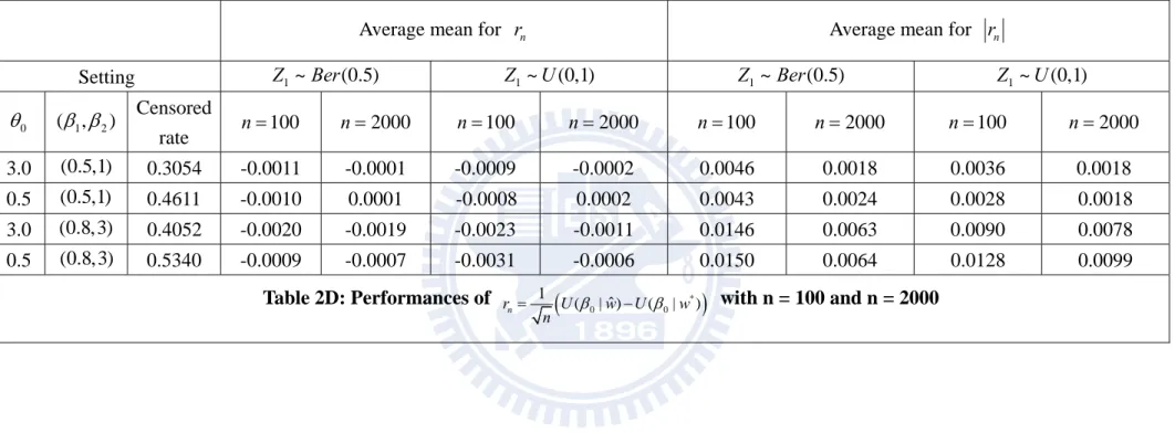
  . We have conducted simulations to check whether ,





*



0 0 1 ˆ ( | ) ( | ) n r U w U w n  

  gets close to zero as the sample size increases. In Table 2D, we

can see that the sample size changes from n100 to n2000, the value of r_n ( or r_n )

decreases and is close to zero.

3.4 Numerical algorithm and variance estimation

The proposed estimators solve ( | )w    1 ( ) ( ) n i i i i       



  1 { ( )} (1 ) 1 ( ) n i i i i          



  ; (3.9a) ( | ) U  w 0 1 { ( ; , )} ( ; ) n i i i Z Z t  w dN t    

_



 , (3.9b) where (1_i   _i _i)w_i and ( , , ) i i w w   S_ ( ) ( ( )) ( ) ( ( )) {1 ( )} i i i i i S S                   

with S_ being replaced by the following explicit formula:

1 1 ( ( ) , 1) ˆ ( ) exp{ } { (1 ) } ( ( ) ) n i i i n u t i i i i i I u S t w I u                  







  .

The estimation procedure requires many iterations by updating the weights using previous estimates. Specifically let w( )m be the m-th step estimate of w based on (ˆ( )m,ˆ( )m ,Sˆ_( )m ). Treating w as fixed value, one can solve ( )m  ( |w( )m ) and 0 U( | w( )m) to obtain 0 ˆ(m1)

( 1) ˆ m

 

respectively and then update

( 1) ˆ m _{( )} S_  t _ 1 ( ) 1 ( ( ) , 1) exp{ } { (1 ) } ( ( ) ) n i i i n m u t i i i i i I u w I u                







  .

3.4.1 Re-sampling based on bootstrap approach

The non-differentiability and the complicated and dynamic weight components make it difficult to derive an analytic formula for variance estimation. The bootstrap approach provides a simulation scheme without extra analytic work. Say R bootstrap samples are drawn from the original data



(X_i, ,_i Z_iT), 1,...,i n



. For each bootstrap sample, we perform the estimation procedure which involves  ( |w( )m ) and 0 U( | w( )m) for say m1,...,M . The sampling distributions of ˆ and ˆ can be approximated based on the K bootstrap estimates. The bootstrap method is time-consuming which involves solving the roots R M times. Note that solving U( | w( )m ) even once is not an easy task. 0

3.4.2 Re-sampling based on pivotal estimating functions

Parzen, Wei and Ying (1994) proposed a re-sampling method which has become a popular tool for variance estimation for many semi-parametric inference problems. This approach is useful when the estimating function is not smooth. In other situations, the derivative of the score function can be derived under some regularity conditions but still contains unknown density functions which cannot be estimated based on the simple plug-in approach.

Now we apply and modify the idea of Parzen et al. (1994). For our problem, the pivotal estimating function are the asymptotic distributions of

* 0 * 0 ( | ) ( | ) w U w            1 1 U        .

Directly applying this approach, we first need to generate many replicates from the pivotal distribution denoted as (_j,U_j) for j1,...,R. Then solve

ˆ ( | { , , }) ˆ ( | { , , }) j j w S U U w S                      _{  }   . (3.9c)

ˆ ˆ j j                      

 , given the observed sample, is asymptotic equivalent to the unconditional distribution

of 0 0 ˆ ˆ                 

  for each j . It implies that the empirical distributions of {( , j j) j1,..., }R

  _,

conditional on the observed sample, can be used to approximate the unconditional distribution of ˆ ˆ

( , )  .

The above procedure, however, is very time-consuming since it still involves many iterations to obtain the solution of (3.9c). We propose to modify the procedure by solving

* * ˆ ( | ) ˆ ( | ) j j w U U w                   , (3.10)

where w denotes the final estimated weight. This modification can avoid the time-consuming ˆ* iterations within each re-sampling run. In Appendix 3, we will see that this modification still produces valid results for variance estimation.

Now we derive the algorithm to simulate random samples from the pivotal distributions. Since our interest is in , we only need to focus on *

( | )

U  w since it does not involve other parameters when _{w is a fixed value. We have} *

* ( | ) U  w * 0 1 { ( ; , )} ( ; ) n i i i Z Z t  w dN t    





 * 0 1 { ( ; , )} ( ; ) n i i i Z Z t  w dM t    



 * 1 ( , ) n i i w    



, (3.10a) where 0 ( , ) { ( ; , )} ( ; ) i w Zi Z t w dM ti

  

_

    . It can be shown that

1/ 2 * 0 ( ; ) ~ _p(0, ) n U  w N _ , (3.10b) where * * 0 0 [ (_i , ) (_i , ) ]T E  w   w

  . Plugging in the final estimated weight, asymptotically we

1/ 2 * 0 ˆ

( ; ) ~ _p(0, )

n U  w N _

, (3.10c)

where the covariance matrix can be estimated by 1 ˆ ˆ ˆ n _{( , ) ( , ) /ˆ ˆ} T i i i w w n       



. (3.10d)

In Section 3.3, we have shown that for  in a small neighborhood of ₀, n U1/ 2 ( | wˆ)n U1/ 2 (₀;wˆ)An1/ 2(  ₀)o_p(1),

where A is the asymptotic slope matrix of n1/ 2U(₀;w*) . We simulate G_i ~N(0,1) independently for i1,...,n. Let ˆ* be the solution to



   _ n i i i G w w U 1 ) ˆ , ˆ ( ) ˆ | (   . (3.10e)

We can show that the conditional distribution of



   n i i i G w n 1 2 / 1 ) ˆ , ˆ (

 , given the observed data, is

also (0, )N_p  . Accordingly the conditional distribution of n1/2(ˆˆ) follows N_p(0,A1A1), which is equivalent to the unconditional distribution of ( ˆ 0)

2 /

1  

n . To implement the

re-sampling algorithm, we repeat (3.10e) for R times and then obtain ˆ*_j for j1,...,R. The sample variance can be used to estimate Var( )ˆ . The proposed re-sampling procedure is much faster than the bootstrap approach since no iteration is needed in solving (3.10e) and also there is no need to deal with the estimating function of .

3.5 Model Checking

We utilize the martingale framework to construct a model checking procedure for the latency distribution. Here the model assumption refers to the chosen form of (.)h . Define the residual process: 1/ 2 1 ˆ ( ; ) ( ; ) n i i i V t  n Z M t   



, (3.11a) where

ˆ ( ; )_i M t  * 0 ˆ ˆ ( ; ) t ( ; , ) ( ) i i i N t  Y u  w d _ u  



  (3.11b) and * 0 1 1 ˆ _{( )} t n _{( ; ) /} n _{( ; , ˆ )} j i i j j t dN u Y u w       

_





 . (3.11c)

The Kolmogorov-type test based on sup_t n1/ 2V t( ; )ˆ can be used to measure the degree of departure from the imposed model.

First of all we need to show that, under the assumed model, V t( ; )ˆ converges weakly to a mean-zero Gaussian process. The argument is similarly to Ghosh (2003). Here we summarize the sketch of proof. One can write

1/ 2 1 ˆ ˆ ˆ ( ; ) ( ; ) n i i i V t  n Z M t   



1/ 2





0 1 ˆ _ˆ ˆ ˆ _ˆ ( ; , ) ( ; , ) n _t i i i n Z Z u  w dM u  w  



 . Notice that 1 1 1 1 ˆ ( ( ) , 1) ˆ ˆ ˆ ˆ _{( ; , ˆ ) ( ( ) , 1) ˆ ( ( ) )} ˆ ˆ ( ( ) ) n j j n n j i i i i i n i i j j j I u M u w I u w I u w I u                    _{ }            _     









    1 1 1 1 ˆ ( ( ) , 1) ˆ _ˆ ˆ ( ( ) , 1) ( ( ) ) ˆ ˆ ( ( ) ) n j j n n j i i i i n i i j j j I u I u w I u w I u                        









    0, for 0 u t.

Using (3.8), V t( ; )ˆ can be rewritten as

1/ 2 _{0 1 0} 1/ 2 ₀ 0 1 ˆ ˆ ˆ ˆ ( ( ; , )) ( ; , ) ( ) ( ) (1) n _t i i n p i n Z Z t  w dM t  w A t n   o      



.

By the martingale central limit theorem and the consistency of ˆ,

V t( ; )ˆ dN_p(0, ) ,

distribution can be approximated by ˆ ( ) V t 1/ 2 * 0 1 ˆ _ˆ ˆ ˆ ˆ { ( ; , )} ( ; ) ( ; ) ( ; ) n _t i i i i n Z Z u  w dM u  G V t  V t   



    . (3.12)

For informal model diagnostics, we can plot the sample curve of V t( ; )ˆ along with several

simulated curves of ˆ ( )V t . If the sample curve is located within the range of simulated curves, the

model assumption is reasonable. Formally, we can generate many replicates of ˆ ( )V t and compute

the value of sup_t n1/ 2V tˆ( ) for the model candidates under consideration. The p-value refers to the empirical frequency that the observed value of sup_t n1/ 2V t( ; )ˆ exceeds the simulated values of sup_t n1/ 2V tˆ( ) .

3.6 Simulation analysis

3.6.1 Data generation

We first generate Z from₁ Bernoulli (0.5)and compute

* (1) * (1)

0 (1, 1) ( 0, 0 ) 0 0 1

T T

Z   Z     Z ,

where the values of ₀* are ₀(1) are specified. Then generate  ~Bernoulli(p_Z) with 0 0 exp( ) ( | ) 1 exp( ) T Z T Z p Z Z        .

If 1  , we generate the latency variable T which follows log T (1) (2)

0 Z1 0 Z2

  

  

where  follows the log-exponential distribution. If  0, we set T to be a very large number exceeding the support of C which follows a uniform distribution. Observed variables include replications of



X, , Z



, where X  T C and  I T C(  ).We consider two settings with A:

) 5 . 0 ( ~ 1 Ber

Z and Z2 ~ Ber(0.5); and B: Z1 ~Ber(0.5) and Z2 ~Unif(0,1).

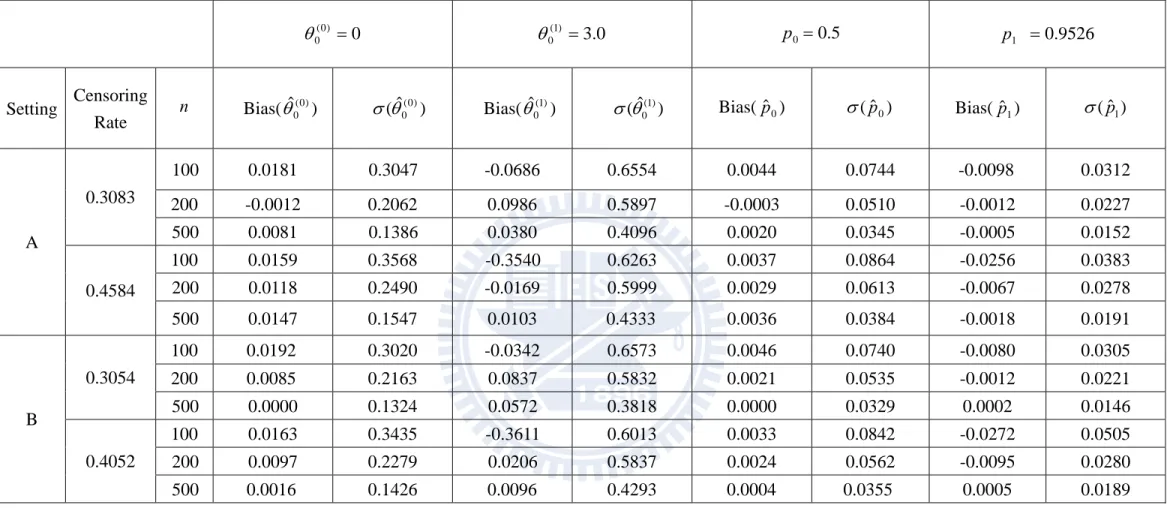
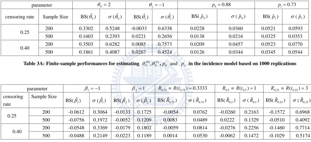
Tables 1A and 1B show the results for estimating ₀(0), ₀(1), (0) 0 0 (0) 0 exp( ) ( | 0) 1 exp( ) p   Z       , and (0) (1) 0 0 1 (0) (1) 0 0 exp( ) ( | 1) 1 exp( ) p   Z           .

We calculate the average bias and standard deviation based on 1000 replications. In the two tables, the estimators have reasonable performances which improve as the sample size increases. Transforming )( , 0(1)

) 0 ( 0 

 into the probability scale based on (p₀,p₁), the performances of

) ˆ , ˆ

(p₀ p₁ look satisfactory. Comparing the two tables which differ in the values of p₁, we see that the corresponding estimator becomes more variable when p₁ is closer to 0.5.

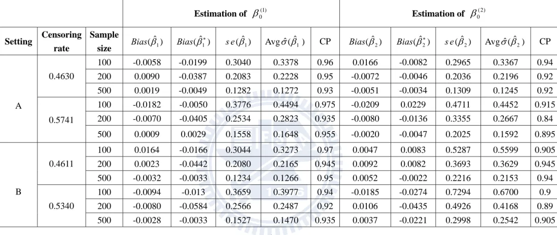
Our main proposal is developed for estimating ₀ in the latency model. Table 2A and Table 2B correspond to the incidence models in Table 1A and Table 1B respectively. The proposed estimators of ₀(1) and ₀(2) have reasonable performances but sometimes produce larger bias when the sample size is small or the censoring rate is high. Our another important proposal is the re-sampling scheme for variance estimation. To examine the performance, we first check whether the sample average of ˆ*_j which solves (3.10e) is close to the true parameter value. Then we examine whether the proposed estimator  ˆ (ˆ_j), which is sample standard deviation of ˆ*_j

(j1,..., )R , is close to the simulated estimate denoted as se(ˆ_j). The results are satisfactory. As a consequence, the coverage probability is close to the 95% nominal level in most cases. Notice that the results in Table 2B appear to be better than those in Table 2A since the former corresponds to higher incidence rate which provides more data to estimate the latency distribution.

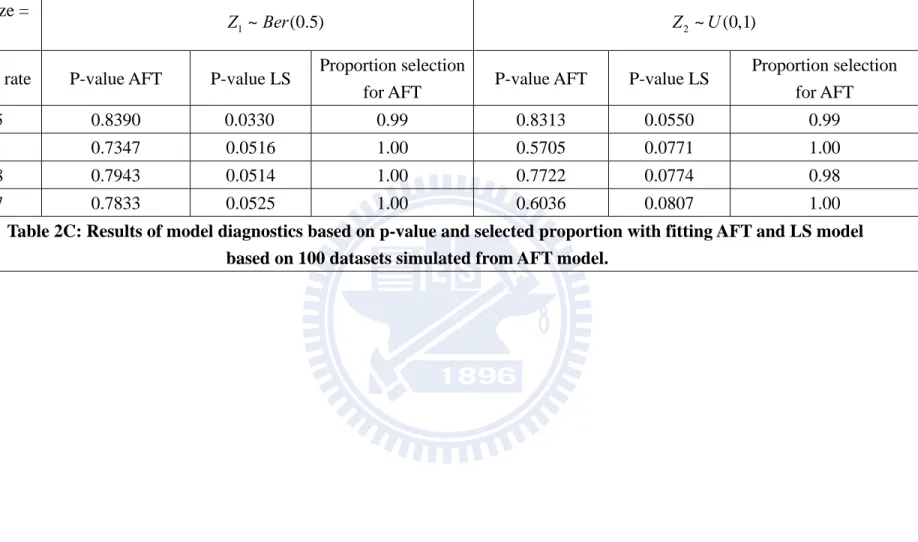
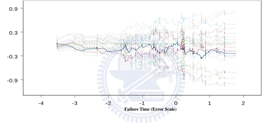
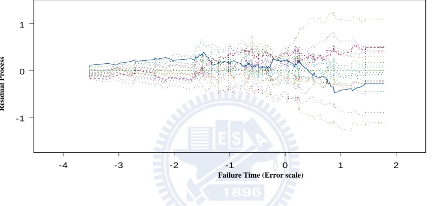
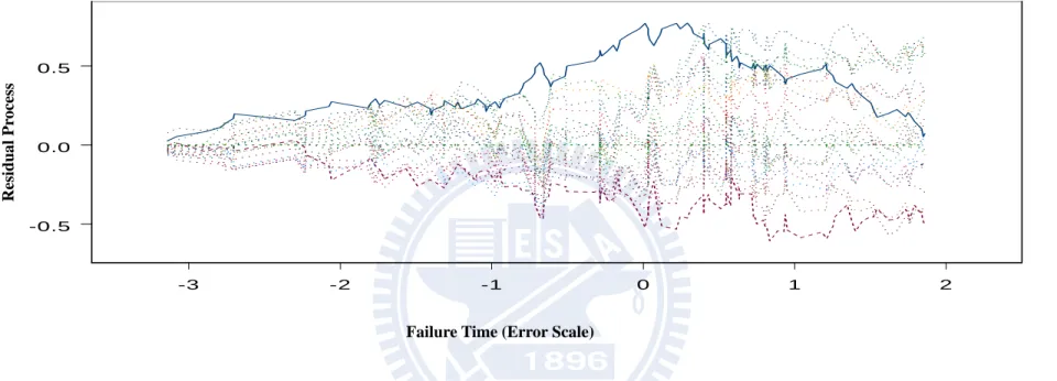
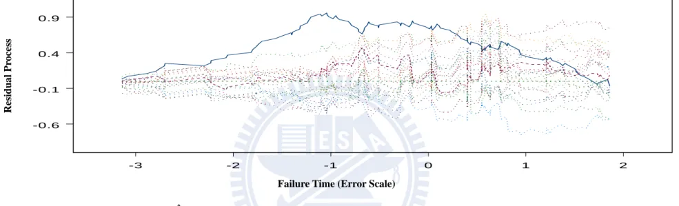
Finally we examine the proposed model checking procedure. We first simulate data from an AFT model and then analyze it by an AFT model. Figures 4.1A and 4.1B show the two

components of V t( ; )ˆ based on Z and ₁ Z respectively. The observed curves are mostly ₂ located within 20 simulated curves which show that the fitted model is acceptable. Then we generate an AFT model and fit a location shift model. Figures 4.2A and 4.2B, the observed curves are located outside the simulated curves which show that the fitted model is not satisfactory.

Chapter 4

Literature Review for

Transformation Models with Cure

4.1 Background

In this chapter we consider the second class of models with the incidence model given by

Pr( 1| )Z  ( ₀| )Z 0 0 exp( ) 1 exp( ) T T Z Z     .

And for   , 1 T follows a transformation model of the form _i 0

( ) T

h T Z   ,

where ( )h  is a unknown monotone function but the distribution of  is completely specified. Note that we denote the distribution, survival and cumulative hazard functions of  as F_, S_ and  which are fully specified. The most well-known example is the proportional hazards (PH) _ model in which  follows the extreme value distribution with F s_

 

1 exp{ exp( )}- - s . When

 follows the standard logistic distribution with F s_ε

 

exp

 

s / + {1 exp

 

s }, the model becomes the proportional odds (PO) model.

For the discussions in this chapter, observed data are denoted as



(X_i, ,_i Z_i), 1,...,i n



, where X_i   and T_i C_i _i I T( _i C_i). The parameters of interest are( , )  while h t is an ( ) infinite-dimensional nuisance function. In the early stage of methodology development, statisticians including Kuk and Chen (1992), Sy and Taylor (2000) and Peng and Dear (2000) focused on the special case that the latency distribution follows the PH model. Then a new trend starting from Lu and Ying (2004) considers statistical inference for the whole of class of transformation models. In this chapter, we review existing literature for transformation cure models. Roughly speaking, existing inference approaches can be classified into two types. One is based on the likelihood principle and the other is based on moment properties.