毫米波無線個人通訊網路適於群播應用之排程演算法

i

國

立

交

通

大

學

網路

網路

網路

網路工程研究所

工程研究所

工程研究所

工程研究所

碩

碩

碩

碩

士

士

士

士

論

論

論

論

文

文

文

文

毫米波無線個人通訊網路適於群播應用之排程演算法

Scheduling for Multicast Services in Millimeter Wave Wireless

Personal Area Networks

研 究 生：詹智涵

指導教授：趙禧綠 教授

中

中

中

中 華

華

華

華 民

民

民

民 國

國

國

國 一百

一百 年

一百

一百

年

年

年 七

七

七

七 月

月

月

月

ii

毫米波無線個人通訊網路適於群播應用之排程演算法

Scheduling for Multicast Services in Millimeter Wave Wireless

Personal Area Networks

研 究 生 : 詹智涵 Student：Chih-Han Chan

指導教授 : 趙禧綠 Advisor : Hsi-Lu Chao

國 立 交 通 大 學

網 路 工 程 研 究 所

碩 士 論 文

A Thesis

Submitted to Institute of Network Engineering

College of Computer Science

National Chiao Tung University

in partial Fulfillment of the Requirements

for the Degree of

Master

in

Computer Science

July 2011

Hsinchu, Taiwan, Republic of China

中華民國一百年七月

iii

毫米波無線個人通訊網路適於群播應用之排程演算法

學生:詹智涵 教授:趙禧綠

國立交通大學網路工程研究所碩士班

摘要

摘要

摘要

摘要

由於近年來對於高速多媒體傳輸的要求變得很受歡迎，IEEE 802.15.3c 訂定了媒體 存取控制與實體層的標準。其實體層的特性包含了使用頻帶在 60GHz ISM 上和波束成 形技術，60GHz ISM 造成了較高的訊號路徑衰退，波速成形技術則是增加了空間重利 用性。從現今應用的角度來看，多媒體資料傳輸較適合以群播方式傳輸。從 Shannon 的 頻寛理論來看，我們可以發現群播資料流的容量和接收者的數目多寡、傳輸者和最遠接 收者的距離、傳輸者的波束角度大小有關。而且，對於每一個群播資料流的接收者選擇 方式將會影響空間的重複利用性。每個群播資料流有 2n -1 種單一分群方式且至少有 2n-1 種可排程之接收者分群集合, n 是接收者個數。我們的目標是針對群播資料流提出一個有 效的連線樣本選擇方式並且結合所提出的公平的排程演算法達到最大化網路效能且不 失去公平性。模擬結果顯示提出的連線樣本方法所選擇的連線樣本在效能上比原本的連 線樣本和全部都拆成單播資料流連線樣本更好，且其效能可近似區域最佳解。和 REX 排 程演算法相比，所提出的排程演算法有較好的效能但也失去一些公平性。

iv

Scheduling for Multicast Services in Millimeter Wave Wireless Personal

Area Networks

Student : Chih-Han Chan Advisor : Hsi-Lu Chao

Institute of Network Engineering College of Computer Science

National Chiao Tung University

Abstract

The high speed multimedia transmission applications had been become popular in recent year, the IEEE 802.15.3c task group had been compose the media access control (MAC) and physical layer (PHY) standard. The physical characteristics include adopting frequency at 60GHz ISM band and beamforming technique which respectively causes high path loss and increases the spatial reusability. In the recent application view, the operation of multimedia data transmission prefers adopt multicast transmission scheme. With the observation of Shannon capacity, we can find out the capacity of a multicast flow is highly correlated with number of receivers (links), distance between sender and receivers and beamwidth of the flow. Also, the link pattern selection of each multicast flow would affect the spatial reusability. Each multicast flow has link flow patterns and at least schedulable link flows set with n receivers. Our objective is to propose an efficient link pattern selection scheme for each multicast flow and joint the fair scheduling algorithm to maximize the system throughput without losing the fairness. The simulation results show that the proposed joint link pattern selection and flow scheduling scheme is better than only unicast link pattern and original link pattern, and the performance approximate to local optimal link pattern selection scheme in throughput. Compare with REX scheduler, the proposed scheduling scheme is better in throughput but with minor loss in fairness.

v

毫米波無線個人通訊網路適於群播應用之排程演算法

學生:詹智涵 教授:趙禧綠

國立交通大學網路工程研究所碩士班

致謝

致謝

致謝

致謝

在研究的這段期間非常感謝家人、同學的陪伴還有老師的指導。過程中經歷了不少 題目的尋找、題目的更換、創新思考、討論到提出方法，每一個步驟都令人刻骨銘心。 雖然每一步都有一些困難與挑戰，但都能以堅持和理性思考方式去解決修正。家人和同 學的陪伴是度過孤獨的最好良藥，老師的指導是不可或缺的加速劑。這一關，我學了耐 心和獨力思考的能力。雖然花了不少時間去學習磨合，但我想應該是值得。

vi

Table of content

摘要 ..………...…...…..………iii

Abstract ...………….……….iv

致謝 .…..….………..……….v

Table of content ………vi

List of Tables ……….……….viii

List of Figures ……….………ix

Chapter 1 Introduction………1

1.1 Characteristics of IEEE 802.15.3c………1

1.2 Motivation and problem descriptions ....…………....………….………2

1.3 Contributions.…..……….……….3

Chapter 2 Related Work ……….………3

Chapter 3 System Model, Antenna Model and Physical Model ………5

3.1 System model and MAC super frame ……….…….5

3.2 Antenna model ……….………6

3.3 Physical model ………..………6

3.4 Derive the beamwidth and azimuth of a multicast flow………...………8

3.5 Derive the mutual cover rule by exclusive region………..10

3.6 The four conflict rules in protocol model……….………..12

Chapter 4 Proposed Link Pattern Selection Scheme and Scheduling Algorithm ………13

4.1 Preliminary……….….13

4.1.1 Conflict graph ...……….………….13

4.1.2 Maximal independent set ………14

4.2 Combination of schedulable link flow set ………..…15

vii

4.4 Design of link pattern selection ……….………17

4.5 Link pattern selection algorithm……….21

4.6 Proposed fair slot assignment (FSA) algorithm……….……….23

Chapter 5 Performance Evaluation……….. 25

5.1 Simulation environment and metric definition………...………25

5.2 Simulation results ……….……..27

5.2.1 Number of flows and system throughput….………27

5.2.2 Minimal beamwidth and system throughput………28

5.2.3 Number of flows and efficiency of merge rule 3………...28

5.2.4 Number of flows and fairness index ………...29

5.2.5 Minimal beamwidth and fairness index ……….……….30

Chapter 6 Conclusion and Future Work ………..31

viii

List of Tables

Table I Description of notations ………...17 Table II Parameters setting ……….………..24

ix

List of Figures

Figure 1-1 The comparison between original link pattern and only unicast link pattern in

scheduling result ….……….………..2

Figure 3-1 Piconet superframe structure ……….………...5

Figure 3-2 The multicast beamforming with beamwidth θ_{………….……….7}

Figure 3-3 The beamwidth and azimuth of a multicast flow ………….………7

Figure 3-4 Illustrations of each type of the multicast flow ………..………10

Figure 3-5 The four confliction rules …………..……….………13

Figure 4-1 Transform the relationship between flows to conflict graph ……….……….14

Figure 4-2 Maximal independent set ………...15

Figure 4-3 Conflict graph of each merge rule …………...………...19

Figure 4-4 Illustration of each merge rule …..…………...………...20

Figure 5-1 Throughput vs number of flows ……….………27

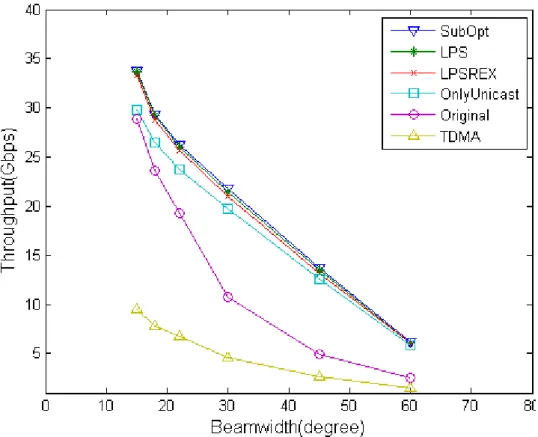
Figure 5-2 Throughput vs minimal beamwidth ………...28

Figure 5-3 Efficiency of merge rule 3 vs number of flows ………..……….29

Figure 5-4 Fairness index vs number of flows ……….………30

1

Chapter 1 Introduction

1.1 Characteristics of IEEE 802.15.3c

Due to the demand of playing high-definition (HD) uncompressed video increases in recent year, the IEEE 802.15.3c task group had been composed the medium access control (MAC) and physical layer (PHY) standard to realize HD video transmissions in Wireless Personal Area Networks (WPAN). To provide at least 1.5Gbps high speed transmission, the main characteristic in physical layer includes adopting operating frequency within 57~66GHz ISM band and the beamforming technique. The natural characteristic of 60GHz and small wavelength leads to high path loss and oxygen absorption which plus beamforming technique would promote the spatial reusability and directivity. In the recent application view, for example likes video conference with augmented reality (AR) technique or 3D applications, it’s better to adopt a new design to support the multicast transmission. There is several existed work discussing about the problem of NLOS flow transmission which is caused by moving obstacle like human. And they proposed multi-hop transmission [3-5] to replace the NLOS single hop transmission. Some other works studies the spatial multiplexing capacity and propose scheduling method based on exclusive region conception. However, as far as we know, there are few researches study the system performance when the unicast and multicast flows coexisted in the WPAN which would be more general in the future.

2

1.2 Motivation and problem descriptions

With the observation of Shannon capacity, the capacity of a flow depends on the distance between sender and receiver, and the main lobe beamwidth of the sender and receiver. A multicast flow includes several receivers in a transmission would increase the multicast flow capacity. However, when there are several multicast and unicast flows in the system, a multicast flow selects more receivers to transmit would enlarge the beamwidth of the multicast flow and cause more collision, which defers other flow transmit together, decreasing the spatial reusability and system throughput. In Figure 1-1, the case 1 contains a multicast flow with sender S1, receiver D1 and D3 and a unicast flow with sender S2 and receiver D2, the multicast flow request 6 time slot and unicast flow request 2 time slot to transmit. The link flows with red color were scheduled in channel time allocation 1 (CTA1) and the link flows with blue color were scheduled in CTA2. Here a link flow is a sender to one or more receivers. First we divide the multicast flow into n unicast link flows and calculate the time requirement of each link flows. In Fig. 1-1 (b), the multicast flow is divided into two unicast flows, with 5 time slot and with 4 time slot, we can find out the flow on original link pattern is better than only unicast link pattern in scheduling result in Fig. 1-1 (c). In Fig. 1-1 (e), coexisted with but collide with . The scheduling result of case 2 shows that only unicast link pattern is better than original link pattern. We can find out the scheduling result is highly correlated with link pattern selection of each multicast flow. It’s the tradeoff between multicast flow capacity and spatial reusability. And my objective is to propose an efficient link pattern selection scheme for each multicast flow and joint it with the scheduling algorithm which is better than the original link pattern and only unicast link pattern in system throughput.

3

1.3

Contributions

The main contributions of the paper are two-fold. First, to the best of our knowledge, the work is the first one to study the system throughput with unicast flows and multicast flows. We propose a link pattern selection scheme and joint it with the proposed scheduling algorithm to achieve the better system performance than the system performance with original link patterns or only unicast link patterns. Also, the system throughput with proposed scheme approximate to the system throughput with suboptimal link pattern selection scheme. Second, the proposed scheme has better system throughput and lower complexity than REX scheduler but with minor loss in fairness.

Chapter 2 Related Work

Due to the special characteristic of mmWave and directional antenna respectively cause high path loss and increase spatial reusability. The authors in [3] proposed exclusive region conception of the receiver to determine if each two flows

Figure 1-1. The comparison between original link pattern and only unicast link pattern in scheduling result

4

can concurrently transmit. The work discusses the exclusive region of the receiver when the sender and receiver both equips with omni-directional antenna or directional antenna, and there are four scenarios. When the sender and receiver both adopt directional transmission, the exclusive region of the receiver contains four zones with one zone like cone shape. Senders of two flows both outside the exclusive region of the receiver of the other flow means the two flows can be coexisted. The authors [4][5] analyze the spatial multiplexing capacity based on the exclusive region concept and the result shows that the most proper exclusive radius is about 4m. Also, the work [4] tells that the smaller the beamwidth of each flow would increase the number of concurrent transmission flows and the spatial capacity of the system. The authors in [6] analyze the probability of a collision occurs in a time slot is about 3.7% in protocol model and 10% in physical model when the interferers were Poisson distributed. And it concludes that the high directive links with mmWave characteristic can be seen as pseudo wired links and the interference in mmWave network can almost be ignored for MAC designer. In [7] and [8], the authors proposed the main idea of multiple high rate hops to replace the low rate hop to enhance the system throughput. The key observation of the work is the distance between transmitter and receiver dominates the transmission rate, so it propose a novel metric which include the hop distance and hop loading as the weight of each hop and the PNC calculates the total weight of each path and select the minimal weighted path for each flow. The proposed scheduling algorithm constructs coexistence groups and allocates each group with maximal flow time of the group. The main problem of the work is the scheduling algorithm doesn’t concern about the later hop in a path can’t not be scheduled before the previous hop which may cause flow starvation of the later hop and it can be improved if it also concern about the coexistence factor between hops of different flows. In [9], the

5

authors proposed the usage of repeater devices to reduce the NLOS effect, the objective of the work is make transmission rate of each flow get up to a threshold, for example 800Mbps, since the selection of a repeater for each flow is NP-hard problem, it proposed a random repeater selection scheme for each flow not get up to the threshold. The main problem of the work is it adopts the random scheme to select the repeater, it’s a time consuming operation because the selection of a flow may reduce the transmission rate of the other flow which already get up to threshold and become no get up to the threshold, some flows may not achieve the threshold in the final because the algorithm stops if it has no more improvement. There are several existed work discuss about how to solve the NLOS transmission problem, but as far as we know, there are little works study the system performance when the unicast and multicast flows coexisted within the mmWave WPAN. The following is the system model and the proposed methods.

Chapter 3 System Model, Antenna Model and

Physical Model

3.1 System model and MAC super frame

In 802.15.3c WPAN, the piconet is constructed on demand. Each piconet contains a piconet coordinator (PNC) and several slave devices. The first device construct the piconet would be the PNC and sent the beacons in the beacon period of a super frame like in Figure 3-1, the other devices get the beacon from the PNC is the slave devices. The super frame contains three periods, beacon period, contention access period (CAP) and channel time access period (CTAP). The channel time access period contains management CTA (MCTA) and data transmission CTA. In beacon period, the PNC sent beacon to synchronize the devices in the system or notify the devices about system information likes scheduling results. In CAP, the newly joined

6

devices can associate with PNC or transmission data with other devices in CSMA/CA manner. In CTAP, the PNC may use the MCTA to send the command or allocate the MCTA to the devices for CTA request. The CTA is used for data transmission in TDMA manner.

3.2 Antenna model

Each node equips with steerable antenna which can direct the beam to any direction with beamwidth range from 0 to . We adopt the ideal flat top antenna model which assumes the radiation of side lobe can be ignored and set null to the direction of interference and noise. The antenna gain of mainlobe is inversely proportional to the mainlobe beamwidth, otherwise, the antenna gain would be zero [5].

(1) is the antenna gain of mainlobe. is the angle difference between vector from sender to receiver and the azimuth of mainlobe.

3.3 Physical model

The transmission rate is derived from Shannon capacity and Friis transmission equation. According to Shannon capacity equation, the achievable data rate is defined as

(2) Figure 3-1. Piconet superframe structure

7

(3) W is the bandwidth, SINR is signal to interference and noise ratio, is the wave length, and is respectively transmission antenna gain and receive antenna gain. is the transmission power, is the distance between transmitter i and receiver j. is the background noise and I is the total power from other concurrent transmitters. is the path loss exponent with value range from 2 to 6. To simplify the complexity, here we assume each receiver have the same interference which is set to background noise. Combine formulation (1), (2) and (3), we can derive the transmission rate of a flow as

(4)

Here the beamwidth of the sender is a variable and beamwidth of the receiver is default minimal beamwidth . When a multicast flow comes with time requirement t, for calculating the time requirement of each unicast link flows of the multicast flow, we can derived it from the equation

(5)

is time requirement of unicast link flow. is the transmission rate of the unicast flow. is the transmission rate of multicast flow. is the time requirement of original multicast flow. is the maximal distance of all receivers of the multicast flow.

3.4 Derive the beamwidth and azimuth of a multicast flow

There are n possible beamwidth for a multicast sender to cover all receivers of the multicast flow. The azimuth of a multicast flow is defined as the transmission direction in the middle of beamwidth which is range from 0 to .

8

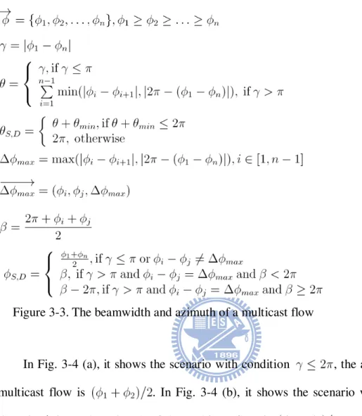
First we get the planar coordination of the receivers of each unicast link flow and transform it to the radian coordination with radian range from 0 to . To derive the minimal beamwidth and azimuth of the multicast flow, we sort the azimuth of each receiver in descendent order as in Fig. 3-3. is the azimuth difference between receiver with maximal azimuth and receiver with minimal azimuth. With condition of , the azimuth of each receiver in the multicast flow must locate within the range . Otherwise, we derive all the azimuth difference with i from 1 to n-1 and , sorting the azimuth difference in ascendent order and get the summation of the first n-1 azimuth difference to take the minimal azimuth difference of the multicast flow. After getting the minimal azimuth difference which cover all the receivers of the multicast flow. For compensating the collision condition of receivers with maximal and minimal azimuth in graph theory, we take the multicast beamwidth with value , if the value larger than , set it to to make sure the beamwidth within . is the maximal azimuth difference between adjacency two links. is the tuple contains maximal azimuth difference of two adjacency links and the azimuth of the two links. is the larger azimuth within and is the smaller azimuth within . is the azimuth of the multicast flow. is in the middle of maximal azimuth and minimal azimuth with condition or . With condition

, the maximal azimuth difference must be and the azimuth of each receiver of the multicast flow must be between and . Otherwise, with condition and , the azimuth of each receiver of the multicast flow must be between cross 0 to and the azimuth of the multicast flow is , set to if is larger than or

9

equal to to make sure the azimuth within .

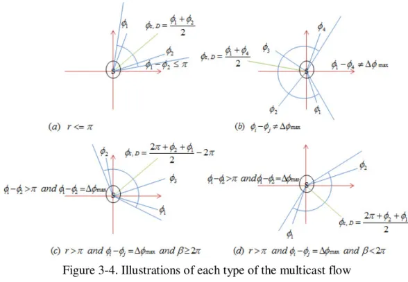
In Fig. 3-4 (a), it shows the scenario with condition , the azimuth of the multicast flow is . In Fig. 3-4 (b), it shows the scenario with condition

, the azimuth of the multicast flow is . In Fig. 3-4 (c), it shows the scenario with condition and and , the azimuth of the multicast flow is . In Fig. 3-4 (d), it shows the scenario with condition and and , the azimuth of

the multicast flow is .

Figure 3-3. The beamwidth and azimuth of a multicast flow

Figure 3-2. The multicast beamforming with beamwidth

10

3.5 Derive the mutual cover rule by exclusive region

To determine if two flows can be coexisted, we would derive the conflict rule called mutual cover rule. The two flows are conflicting when sender of the two flows is covered by the receiver of the other flow. The following is the process to derive the mutual cover rule.

The interference from one of concurrent flow is the received power from the sender of the other flow and it set as Friis transmission equation [10].

(6) is the received power of receiver j and is the distance between

interferer k and receiver j. The total interference from n concurrent flows show as (7) And we set the interference value less than the background noise to match our assumption. We calculate the exclusive region conservatively and set the distance of all n interferer equal to the distance which the closest interferer has. Convert the equation (7) to

11

(8) is the minimal distance between receiver j and maximal interferer k. The exclusive distance of receiver j would be

(9)

In general, when and n is limited. The exclusive radius . The scenario of (9) show the case when the interferer is within the mainlobe of the receiver and the receiver is also within the mainlobe of the interferer. When the interferer is within the mainlobe of the receiver and the receiver is outside the mainlobe of the interferer, the interference is derived as

(10) When the receiver is within the mainlobe of the interferer and the interferer is outside the mainlobe of the receiver, the interference is derived as

(11) When the interferer is outside the mainlobe of the sender and the interferer is outside the mainlobe of the receiver, the interference is derived as

(12) In the condition of (10), (11) and (12), we get the relationship of exclusive distance as

12

In general, and n is limited, the exclusive distance would close to zero with radian . With the equation (9) and (13), we get the mutual cover rule likes Fig. 3-5 (a).

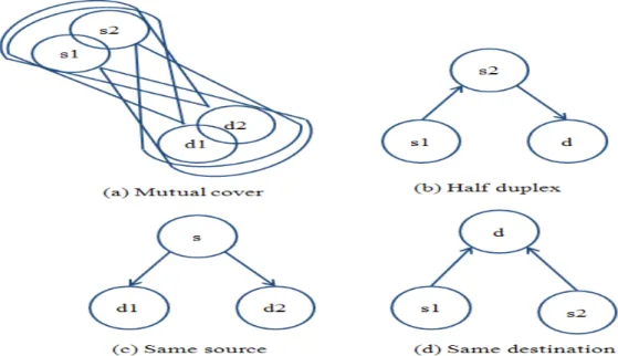
3.6 The four conflict rules in protocol model

There are four conflict rules to determine the conflict condition between two flows which respectively show in Fig. 3-5. The first one in Fig. 3-5 (a) is the mutual cover, when a receiver was covered by the main beam of the interferer and the interferer is also covered by the main beam of the receiver, the confliction occurs. The second one in Fig. 3-5 (b) is the half duplex which means one device can’t transmit and receive at the same time. The third one in Fig. 3-5 (c) is the flows from one device can’t be simultaneously transmitted. The fourth one in Fig. 3-5 (d) is two flows can’t transmit to the same destination at the same time. The mathematic formulation of each conflict rule is presented as following.

Mutual cover: and

Half duplex: and Same source:

Same destination:

represents the angle difference between azimuth of flow i and the vector from

si to receiver j of the other flow. is the beamwidth. is the destination set of flow i.

13

Chapter 4 Proposed Link Pattern Selection

Scheme and Scheduling Algorithm

In section 4.1, we would show the preliminary before start our proposed schemes. In section 4.2, we would show the combination of link flows sets. In section 4.3, we would prove the minimal time frame length scheduling problem is a NP-hard problem. In section 4.4, we would discuss the design of link patterns selection. The link patterns selection algorithm was presented in section 4.5. The proposed fair slot assignment algorithm was presented in section 4.6.

4.1 Preliminary

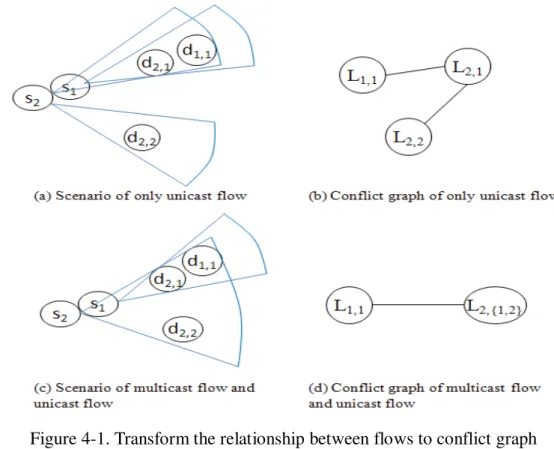
4.1.1 Conflict graph

In the conflict graph, a node represents a link flow and an edge between two nodes represents the two link flows are conflicted. We would split the multicast flow into the number of destination unicast link flows and transform the problem into conflict graph. Each node in the conflict graph is a unicast link flow at initial state. The edge between two nodes means two link flows can’t be coexisted. Since we would merge two nodes into one node in the conflict graph, we define the merge link

14

flows set {ML}. Each link flow in the set {ML} may be a unicast link flow or a multicast link flow. We construct the conflict graph base on the four conflict rule described in section 3.6. For example in Fig. 4-1 (c), the flow of S2 is a multicast flow with destination d2,1 and d2,2 and it split into two unicast link flows like Fig. 4-1 (a). In Fig. 4-1 (b), L1,1 represents the link flow S1 to d1,1, L2,1 represents the link flow S2 to d2,1, L2,2 represents the link flow S2 to d2,2, since L1,1 conflict with L2,1 base on mutual cover rule, and L2,1 conflict with L2,2 base on same source rule, there exists an edge between them in conflict graph. The same rules show in Fig. 4-1 (c)-(d), since it’s a multicast link flow of S2, if one of its unicast link flow conflict with the other link flow in {ML}, it means the two link flows were conflicted.

4.1.2 Maximal independent set

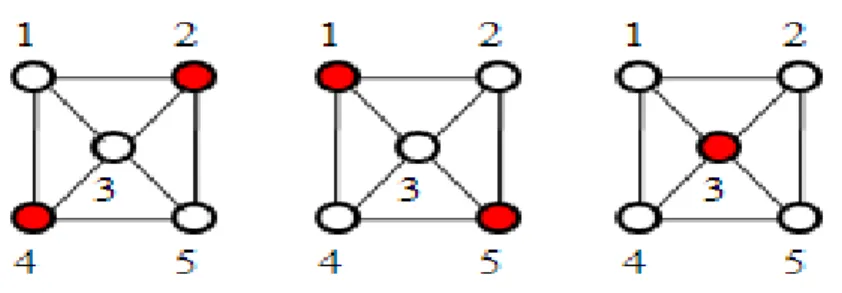
In graph theory, a maximal independent set (MIS) or maximal stable set is an independent set that is not a subset of any other independent set. For example, we have {b}, {a,c} two MISs, then {a} is not a MIS since it was a subset of {a,c}. Figure

15

4-2 shows all the MISs of the five nodes, {2,4},{1,5},{3}.

4.2 Combination of schedulable link flows set

Each multicast has 2n-1 link patterns. n is the number of destinations of the multicast flow. The number of schedulable link flows of each flow is derived as

(14) The total number of schedulable link flows set is derived as

(15)

N is the number of the flows in the system. Since the combination of schedulable link flows set is exponential, we would propose an efficient link pattern selection scheme for each multicast flow and select a good schedulable link flows set compare with the original link flows set and only unicast link flows set. The link pattern selection problem is highly correlated with scheduling problem and it would affect the final scheduling result.

4.3 Proof of minimal time frame length scheduling problem is

NP-hard

We could transform the schedulable link flow set into conflict graph and find the maximal independent set to schedule in each slot. First we proof the minimal time frame length scheduling problem is a NP-hard problem and it also can be formulate as ILP problem which is also a NP-complete problem.

Theorem 1.0. In a general conflict graph, the minimal time frame length scheduling problem is a NP-hard problem.

16

Proof. To minimize the time frame length, it should schedule maximum independent set of the conflict graph in each time slot. For instance, given a conflict graph G with two nodes and find a maximum independent set in graph G. We could reduce the problem to minimal time frame length problem. We create the G’ which is equal to G and set the time requirement of each node in G’ to 1. To find a maximum independent set in G if and only if solving the minimal time frame length scheduling problem in

G’. G reduces to G’ is a polynomial time reduction.

We formulate the minimal time frame scheduling problem as integer linear programming (ILP) problem.

(16) is the set of maximal independent set after we select a schedulable link flow set. is the number of time slot allocated to MIS . The ILP problem is a NP-complete problem and the complexity is too high for practical system to adopt.

We define each entry of the concurrent link set of , CLS( ), as a set of link flows coexist with . We prove each link flow L belong to entry of set of maximal independent set (SMIS) of , SMIS( ), implies L belong to CLS( ).

Lemma 1.0. Proof.

17

4.4 Design of link pattern selection

We defined the relational symbols in Table I. We would split each multicast flow into multiple unicast link flows, transform it to the conflict graph and merge selected two link flows into one link flow called merged link flow Li,J _{depends on the}

defined benefit B. To solve the general case in conflict graph, we class the graph into one of following three classes with corresponding merge rule. The merge rule 1 is when the merged link flow _{coexist with and} , we set the benefit to . Figs. 4-3 (a),(b) show the scenario of class one,

and are unicast link flows of a multicast flow, coexist with which is included in _and . Actually, there exists multiple scenarios include in each of three classes. The benefit is defined as predicted difference of scheduling result between before merge and after merge, and if the benefit is larger than zero, the link pattern selection operator would merge the selected

Table I. Description of notations

Notations Description

{ML} Merge link flows set.

V represents link flows and E represents conflict relationship.

A set of link flows coexist with . (CLS)

_{A set of link flows conflict with . (NS)}

Maximal independent set of . (MIS)

Set of maximal independent set of . (SMIS)

A set of link flows conflict with and . (CNS)

Original graph G delete the and

After merge of original graph G and delete the and

Bi

The defined benefit of merge rule i. It was defined as predicted difference of scheduling results between before merge and after merge.

18

two link flows _{and into} . Here we explain the definition of merge rule 1. If a scheduler A schedule the other merge link flows except the selected two link flows, the scheduling result is the same between before merge and after merge. After that, the predicted difference of before merge and after merge would be

since coexist with each entry of and

which means _{coexist with each entry of and} , _could be scheduled with each entry of _and .

The merge rule 2 is when the merge link flow _{conflict with but}

coexist with , . The

time requirement of _{must be larger than} and _{since the transmission} rate of multicast flow is less than or equal to minimal transmission rate of unicast link flow of the multicast flow. First we delete the _{from the graph of before merge} and schedule the {ML} of before merge and {ML} of after merge. The difference of scheduling result is equal to , after that attach _{back to graph of} before merge and schedule it. The benefit of merge operation is the additional cost in

before merge and the benefit would be , for

simplicity, we take the as the benefit of merge operation. Figs. 4-3 (c), (d) show the scenario of class 2.

The third scenario is when _{conflict with} and . In this case, we would cut some nodes in graph of before merge and after merge which would not affect the difference of scheduling result. There are three types of nodes except the selected nodes _and . The first type _{is the co-conflict nodes} which conflict with and in the graph of before merge. In Fig. 4-3 (e), the node L4,1 is belong to . With the condition one that coexist with other nodes

19

we can delete the co-conflict nodes without affecting the difference of scheduling result. Since the co-conflict node fulfill the condition one, would be included in maximal independent set (MIS) of , the difference of scheduling result would not change after we delete the nodes in type . The second type is the co-concurrent node which coexist with and its value is less than or equal to , for example likes in Fig. 4-3(e). Since

and is included in SMIS of , the scheduler allocate time slot to in before merge or allocate time slot to in after merge is equal to simultaneously allocate time slot to , so we can delete the _{without affecting the difference of} scheduling result. The final step is scheduling the flows in remaining graph of before merge and after merge, take the difference as the benefit of merge rule 3. The following is the steps we calculate the benefit of merge rule 3.

When _{conflict with} and _.

(1) With condition that coexist with other merge link flows except _and 1

,j+

i

L _and . Delete from

graph of before merge and after merge.

(2) With condition that coexist with _and , . Delete from graph of before merge and after merge.

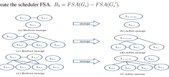
(3) Create the scheduler FSA. .

20

In Fig. 4-4 (a), it contains a unicast flow L2,1 with 3 time slot and a multicast

flow L1,{1,2} with 5 time slot and it was split into two unicast link flows respectively

L1,1 with 5 time slot and L1,2with 4 time slot. The scheduling result of after merge is 5

time slot which is better than before merge. By the merge rule 1, the benefit B1=

5+4-5 = 4 which is larger than zero. In Fig. 4-4 (c), it contains a multicast flow L1,{1,2}

with 9 time slot, a unicast flow L2,1 with 5 time slot and a unicast flow L3,1with 4 time

slot. By the merge rule 2, the benefit B2=7-9+max(9-5,0)=2 which is larger than zero.

In Fig. 4-4 (e), it contains a multicast flow L1,{1,2} with 9 time slot, a unicast flow L2,1

with 7 time slot, a unicast flow L3,1 with 6 time slot and L4,1 with 5 time slot. By the

merge rule 3, we could delete co-conflict node L3,1 and co-concurrent node L4,1

without affecting the difference of scheduling results between before merge and after merge.

21

4.5 Link pattern selection algorithm

First we get the unicast and multicast flow requests with time requirement T. The link pattern selection module would split each multicast flow into multiple unicast link flows with new time requirement fulfill the same data size of the original multicast flow. {ML} is the merge link flows set which contains only unicast link flows at initial state. After the operation of LPS, the set {ML} may contain unicast link flows and multicast link flows. We design the LPS based on the local climbing method. The merge rules are the simple search scheme to the better state compare with the previous state. The time complexity of LPS is . After the operation of LPS, we would schedule the selected link flows set with proposed scheduling algorithm. The following is the proposed LPS algorithm.

• Input: Unicast link flows set {ML}

• Step 1: Sort {ML} by time requirement in descendent order.

• Step 2: Find S_{1 and S2 of each unicast link flows. Select of one multicast} link flows from second entry to last entry in {ML}.

• Step 3: Search _{of the same multicast flow from first entry of {ML} to entry} before . If exists, check the merge rule and invoke the merge function if pass one of the merge rule.

Merge function: update S1 and S2 of S1 (Li,J ) and S2 (Li,J ).

1. Delete _and from S2 of S2 (Li,J ) and add _{to S}2 of S2 (Li,J ).

2. Delete _{and from S}1 of S1 (Li,j ) and S1 (Li,j+1 ).

3. Add to S1 of S1 (Li,J ).

4. Delete and from {ML}. 5. Add to {ML} in sorted order.

• Step 4: Create _{by merge and and create S1 (Li,J ) and S2 (Li,J ).} Merge rule 1:

22

1. If coexist with S1 (Li,j ) and S1 (Li,j+1 )

2.

3. If , invoke merge function and goto step 5. Merge rule 2:

1. If _{coexist with S}1 (Li,j+1 ) and conflict with S1 (Li,j ).

2.

3. If , invoke merge function and goto step 5. Merge rule 3:

1. If conflict with S2 (Li,j ) and S2 (Li,j+1 ).

2. If coexist with other flows except and and . Delete from graph of before merge and after merge.

3. If coexist with _and , . Delete from

graph of before merge and after merge.

4. Create the scheduler FSA. .

5. If , invoke merge function and goto step 5. • Step 5: Repeat step 3 and step 4 until finish a round.

23

4.6 Proposed fair slot assignment (FSA) algorithm

As mention in section 4.3, we prove the minimal time frame length scheduling problem is NP-hard. To reduce the time complexity and achieve high throughput and fairness, the proposed scheduling scheme gives high priority for flows with minimal allocated time and maximal time requirement to schedule first. In the conflict graph view, we always select the concurrent flows with large time requirement which maximize the CTAP utilization of allocated slots. The time complexity of FSA is . The complexity of sorting operation is and the number of operation in slot allocation is , F is the maximal time requirement which is a constant number and the time complexity of FSA would be . The proposed FSA algorithm is presented as algorithm 1.

24

Algorithm 1: Fair Slot Assignment Algorithm

Input: Merge link flows set {ML} with n flows and allocated time and time requirement Ti of each flow i.

1: Create slot set {S}.

2: Create a merge link flows set

3: Sort {ML} by time requirement in descendent order 4: While size of {ML} 1

5: Find minimal allocated time flow . 6: Create a new slot ;

7: Clear ; 8: If (size of {ML} == 1) 9: ; 10: Add to ; 11: If ( ) 12: Remove from {ML}; 13: End If 14: Add to {S}; 15: Continue; 16: End If 17: For in {ML}, i = 1 to 18: If

19: If concurrent with all flows in _{(pass four conflict rules)} 20: Add _to ; 21: Else 22: Add _to ; 23: End If 24: End for 25: For in , i = 1 to

26: If concurrent with all flows in _{(pass four conflict rules)} 27: Add _{to ;} 28: End For 29: For in , i = 1 to 30: ; 31: If ( ), remove from {ML}; 32: End For 33: Add to {S}; 34: End while 35: Return size of {S}

25

Chapter 5 Performance Evaluation

5.1 Simulation environment and metric definition

To match the practical environment the WPAN deploy in, we set the topology as 10m x 10m indoor office room. In the WPAN system, the flows were generated with random source and destination, and we alternatively add the multicast and unicast flow to the system. Each flow has time requirement random from 1s to 10s. The multicast flow contains random number of destination from 2 to 5. The other parameters are setting as table II. To calculate the time requirement of unicast link flow of the multicast flow, we get it from and take the ceiling of . We take the SubOpt with FSA, LPS with FSA, LPSREX, OnlyUnicast with FSA, Original with FSA and Original with conventional TDMA scheduler in comparison. The SubOpt is a local optimal link pattern selection scheme and we derive the schedulable merge link flows set by recursively take two merge link flows of a multicast to merge if the scheduling result is better. LPS with FSA is our proposed link pattern selection and scheduling scheme. LPSREX is LPS cooperate with REX scheduler [5]. The metrics we concern about is throughput and fairness. We formulate the system throughput as

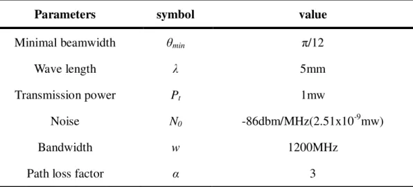
Table II Parameters setting

Parameters symbol value

Minimal beamwidth θ_min π_/12

Wave length λ 5mm

Transmission power Pt 1mw

Noise N0 -86dbm/MHz(2.51x10-9mw)

Bandwidth w 1200MHz

26

(17) is transmission rate of flow i. is time requirement of flow i. is number of destination of flow i. N is total allocated time in the system. To measure the impact of the operation of deleting flows in merge rule 3, we define the efficiency of merge rule 3 as

(18)

N is number of link flows before merge rule 3, is the number of link flows after merge rule 3, the power two is proportional to the complexity of scheduling scheme. To measure the fairness between scheduling schemes, we define the Jain fairness index as

(19)

is the allocated time for flow i. The fairness index is calculated when total allocated time is larger than half the total time requirement.

27

5.2 Simulation results

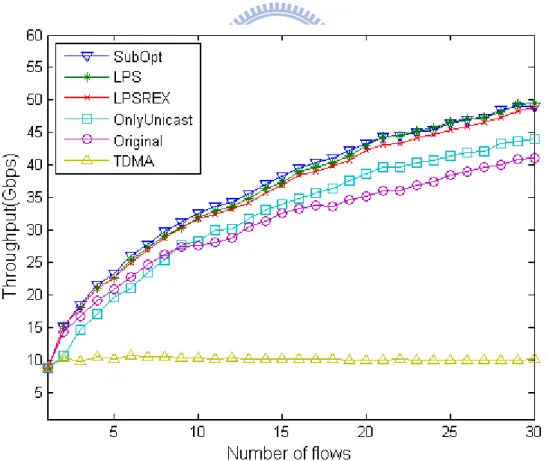
5.2.1 Number of flows and system throughput

In Figure 5-1, when the number of flows increases, it has the better spatial reusability and the throughput also increases. The link flows set selected by proposed LPS scheme is better than the only unicast link flows set and original link flows set. Also, it is approximate to suboptimal link pattern selection scheme. FSA is better than REX scheduler in throughput. When the number of flows is small, the original link flow set would be better than only unicast link flows set since the conflict probability derived from mutual cover is low and the conflict factor is mainly dominated by the same source rule. The multicast flows avoid the same source rule and make more spatial reusability. Inversely, when the number of flows increases, the mutual cover rule would dominate the spatial reusability.

28

5.2.2 Minimal beamwidth and system throughput

In Figure 5-2, we can find out the throughput decrease when the minimal beamwidth increases. The larger the minimal beamwidth lead to lower transmission rate of each flow and lower spatial reusability. The LPS is better than the others and approximate to SubOpt. When the minimal beamwidth enlarge, the LPS prefer not merge since there is no spatial reusability if it merge to multicast flows. We also can find out the original link flow set with FSA almost become conventional TDMA scheduling state when the minimal beamwidth is about 60 degree.

5.2.3 Number of flows and efficiency of merge rule 3

In Figure 5-3, the flow deletion operation in merge rule 3 reduce almost half the time complexity compare with SubOpt link pattern selection scheme when the number of flows large enough. When the number of flow less than ten, because the high spatial reusability lead to small number of co-conflict flows. It’s not harmful since we should take more concern about the scenario with large number of flows.

29 5.2.4 Number of flows and fairness index

We calculate the fairness index when the total allocated time larger than half the total time requirement of all flows. In Figure 5-4, we can take the conventional TDMA scheduling scheme as the upper bound in fairness index. The LPSREX is better than the others since it always schedule the flows with smallest allocated time first. The proposed FSA loss some fairness but keeps higher throughput and lower time complexity. The complexity of REX scheduler is , N is number of flows, since it iteratively sorting the flows for scheduling the flows with minimal allocated time. The fairness index decrease when number of flows increases, it’s because it has more flows with small time requirement scheduled before we take the fairness index value.

30 5.2.5 Minimal beamwidth and fairness index

In Figure 5.5, there is litter difference in fairness when the minimal beamwidth increases. The larger the beamwdith make larger difference in time requirement between multicast flows and unicast flows, and it also reduces the spatial reusability. The difference would decrease the fairness since some small time requirement flows (unicast flows) has been scheduled before we take the value.

Figure 5-4. Fairness index vs number of flows

Figure 5-5. Fairness index vs minimal beamwidth

31

Chapter 6 Conclusion and Future Work

In this work, with the motivation of the multicast data transmission paradigm is more suitable for multimedia multicast applications and the scheduling result is highly correlated with link pattern selection of multicast flows and the cooperated scheduler, we proposed a link pattern selection (LPS) scheme which transform the link pattern selection problem into conflict graph and find some rules to merge the link flows to the better state. In merge rule 3, we delete the flows to reduce the time complexity and approximate to suboptimal link pattern selection scheme in throughput. We also proposed the fair slot assignment (FSA) scheduling algorithm which maintains the fairness without throughput reduction. From the simulation results, the proposed LPS with FSA is better than the others and approximate to suboptimal scheme in throughput but with minor loss in fairness than LPS with REX scheduler. To get up to more practical scenario in WPAN system, we would take the NLOS problem into consideration in the future work.

32

References

[1] "IEEE Standard for Information technology - Telecommunications and information exchange between systems - Local and metropolitan area networks – Specific requirements Part 15.3: Wireless Medium Access Control (MAC) and Physical Layer (PHY) Specifications for High Rate Wireless Personal Area Networks (WPANs) Amendment 1: MAC Sublayer," IEEE Std 802.15.3b-2005 (Amendment to IEEE Std 802.15.3-2003) , pp. 0_1-146, 2006.

[2] "IEEE Draft Amendment to IEEE Standard for Information technology-- telecommunications and information exchange between systems— Local and metropolitan area networks--Specific requirements--Part 15.3: Wireless Medium Access Control (MAC) and Physical Layer (PHY) Specifications for High Rate Wireless Personal Area Networks (WPANs): Amendment 2: Millimeter-wave based Alternative Physical.

[3] L. X. Cai, L. Cai, X. Shen, and J. W. Mark, "Efficient Resource Management for mmWave WPANs,'' Proc. IEEE Wireless Communications and Networking Conference (WCNC'07), Hong Kong, Mar. 2007.

[4] L. X. Cai, X. Shen, L. Cai, and J. W. Mark, “Spatial Multiplexing Capacity Analysis of mmWave WPANs with Directional Antennae,” Proc. IEEE Globecom'07, Washington, DC, Nov./Dec. 2007

[5] L. X. Cai, L. Cai, X. Shen, and J. W. Mark, “REX: a Randomized EXclusive Region based Scheduling Scheme for mmWave WPANs with Directional Antenna” IEEE Trans. Wireless Commun., Vol. 9, No. 1, pp.113-121, 2010 [6] R. Mudumbai, S. Singh, and U. Madhow, “Medium access control for 60 GHz

outdoor mesh networks with highly directional links,” in Proc.IEEE INFOCOM 2009, Mini Conf., Rio de Janeiro, Brazil, Apr. 2009.

[7] Jian Qiao, Cai, L.X., Xuemin Shen, "Multi-Hop Concurrent Transmission in Millimeter Wave WPANs with Directional Antenna,” Communications (ICC), 2010 IEEE International Conference on, pp1 – 5, 23-27 May 2010

[8] Zhou Lan; Sum, C.-S.; Wang, J.; Baykas, T.; Jing Gao; Nakase, H.; Harada, H.; Kato, S.; “Deflect Routing for Throughput Improvement in Muti-hop Millimeter-Wave WPAN System”, in IEEE Wireless Communications and Networking Conference (WCNC) 2009.

[9] Yiu, C. ; Singh, S. ; “Link Selection for Point-to-Point 60GHz Networks” Communications (ICC), 2010 IEEE International Conference on, pp1 – 6, 23-27 May 2010

[10] Http://www.ieee802.org/11/Reports/tgad_update.htm.“11-09-0334-08-00ad-chan nel-models-for-60-ghz-wlan-systems”