生態系統中恢復率的計算

國 立 交 通 大 學

應用數學系

碩

士

論

文

生態系統中恢復率的計算

Computations of Recovery Rates in Some

Ecological Systems

研 究 生：李柏瑩

指導老師：石至文 教授

國 立 交 通 大 學

應用數學系

碩

士

論

文

生態系統中恢復率的計算

Computations of Recovery Rates in Some

Ecological Systems

研 究 生：李柏瑩

指導老師：石至文 教授

生態系統中恢復率的計算

Computations of Recovery Rates in Some

Ecological Systems

研 究 生：李柏瑩 Student：Bo-Ying Lee

指導教授：石至文 Advisor：Chih-Wen Shih

國 立 交 通 大 學

應 用 數 學 系

碩 士 論 文

Submitted to Department of Applied Mathematics College of Science

National Chiao Tung University in Partial Fulfillment of the Requirements

for the Degree of Master

in

Applied Mathematics June 2009

Hsinchu, Taiwan, Republic of China

誌 謝

首先，感謝我的指導教授石至文老師，在研究所的期間所給予

在課業方面的教導以及未來人生方向的指引。同時引領我進入做

研究的世界，讓我對數學研究工作有了更進一步的理解，也對我

無論在數學以及其他的層面上都有著深刻的啟發。在此也感謝所

有口試委員，給了許多寶貴的建議，讓我的論文能夠更加完整。

另外也要感謝成長的路上所有曾經教導過我的老師們，激發我對

數學的好奇心，讓我能夠有機會踏入數學領域。同時感謝所有學

長姐以及同學朋友們，謝謝各位所給予的支持與鼓勵，讓我有繼

續做研究的動力。然而，在論文撰寫過程中特別感謝所有研究室

的夥伴們:哲皓、文昱、瑞毅、奕伸、義閔、光祥、鼎三、芳竹、

俊銘，因為你們的陪伴讓研究所的生活增添了許多的色彩也因此

留下許多美好的回憶。

最後，我要感謝我的家人，因為有你們在成長的路上的支持與

陪伴，讓我能夠順利的完成這篇論文。此份榮耀我要與你們分享，

謹以此文表達我最誠摯的謝意。

生態系統中恢復率的計算

學生：李柏瑩 指導老師：石至文 教授

國立交通大學應用數學系(研究所)碩士班

摘 要

生態系統中變化的發生往往沒有明顯的徵兆。因而需要一個有效

的方式以預測變化的發生。近來眾多研究者提出環境恢復力的下降可

提供變化即將來臨的預兆;但是，在實際上環境的恢復力是難以量測

的，於是需要一些間接的指標以測量環境的恢復力。最近的一些研究

文獻顯示臨界慢化是一個良好的環境恢復力的指標。在這篇報告裡頭

我們運用分析以及數值的方法刻劃了幾個關於捕食者與獵物模型，三

個物種的食物鏈模型，以及基因控制模型的結果。這些結果將引領我

們預測在更多物種的生態學模型或真實世界變化的發生。

Computations of Recovery Rates in

Some Ecological Systems

Student : Bo-Ying Lee

Advisor : Chih-Wen Shih

Department of Applied Mathematics

National Chiao Tung University

Hsinchu, Taiwan, R.O.C.

June 2009

Abstract

Transitions in ecological systems often occur without apparent warning. Thus an effective way of prediction is in strong demand. Recent researchers proposed that decreasing ecological resilience can signal an upcoming transi-tion. Unfortunately, it is very difficult to measure the resilience in practice. Therefore, we need some indicator to measure it. Some recent works in the literatures investigated that critical slowing down is a good indicator of eco-logical resilience. In this report, we use analytical and numerical methods to characterize several results about two-species generalized predator-prey model, three species food chain model, and generic control system. These results can lead directly to predict more complex systems in ecology or real world.

Contents

1 Introduction 1

2 Some basic definitions and classical theorems 3 3 Generalized predator prey model 6 4 Three species food chain model 12

1

Introduction

It is very important to predict the transition in ecosystems. However, the transitions are often difficult to predict, because they can originate from a variety of factors. Decreasing ecological resilience has been proposed as a signal of upcoming transi-tions in complex systems [6, 7]. Ecological resilience is the ability of a system to absorb perturbations and persist at a particular stable equilibrium [3, 5]. In other words, this is a measure of how much that parameter would need to be perturbed to reach the threshold point, and it correlates to the size of the basin of attraction. Unfortunately, ecological resilience can not be measured directly in practice, so there is a need for indirect indicators. One such potential indicator is “critical slowing down”, the decrease in recovery rate that occurs as the basin of attraction around a stable equilibrium contracts and a system approaches a transition [5]. For a variety of ecological models, critical slowing down often occurs far enough from a threshold to be a potentially useful indicator of an upcoming transition [5]. Most importantly, this phenomenon can be proved mathematically to occur as all continuous differ-ential equations approach local bifurcations [4]. Recovery rates are inferred from the amount of time that the system needs to return to equilibrium after a small perturbation [5]. But, it is also not so easily quantified, even in models. Hence, we demand some method to estimate the quantity of recovery rates for any system. Fortunately, the recovery rate can be determined by linearizing at the stable equi-librium and determining the eigenvalues in a model, since the dominant eigenvalue is an approximation of the recovery rate to equilibrium [17, 18].

For each model, we then calculate the recovery rate as the absolute value of the real part of the dominant eigenvalue λdom of the Jacobian matrix at each stable

equilibrium (the dominant eigenvalue is the eigenvalue with greatest real part for a continuous system) [5, 19]. The first step in the analysis of each model is to find its equilibria and the conditions for existence and stability of these equilibria. To find the conditions for stability we linearize each model around its equilibria by constructing the Jacobian matrix and applying the Routh-Hurwitz criteria for two dimensional and three dimensional continuous-time systems. In this report, we estimate the recovery rates by linearizing the models and determining the maximal real part of the eigenvalues of the Jacobian matrix.

However, we are interested in measuring the distance between the point at which the recovery rate starts to decrease Kr and the critical transition Kcrit. This

distance can be seen as a warning period of the upcoming transition. The utility of critical slowing down as a leading indicator of the transition depends on the length of this warning period. Our method can yield general conclusions about the effects of the various parameters on the usefulness of critical slowing down as an indicator of an upcoming transition in a systems dynamics.

Critical slowing down has been proposed as a leading indicator of transitions in real world [5]. In 2007, Van Nes and Scheffer showed using numerical techniques that critical slowing down occurs far enough from a transition to be a promising indicator of loss of resilience for several ecological models. Van Nes and Scheffer are only the first steps towards establishing when critical slowing down will be a useful leading indicator of transitions in different ecosystems. In the last few years, several articles have been devoted to the study of the relationship between critical slowing down and ecological resilience. In this report, we choose these models because they are the simplest and most studied in biology. Of course, we can extend these insights to more complex, multi-species systems and predict that critical slowing down is still an effective indicator. Here, we just give slight theoretical contributions. Our study in this report is just a stepping stone to understanding more complex ecological models. To understand them, we require more mathematical theories than we have used here.

Moreover, there are various concepts and terminology from dynamical systems that we use in this report. These concepts are usually covered in an undergraduate (or graduate) course in ordinary differential equations. Here, we summarize these basic theory in Section 2. For a more complete treatment and more details, see [1, 2, 8, 9, 10, 11, 12, 13, 14].

2

Some basic definitions and classical theorems

In this section, we collect some basic definitions and classical theorems in ordinary differential equations that we will use in this report. Consider the nonlinear system

˙x = f (x), f ∈ C1_(Rn_).

Let φt be the flow map for the system.

Definition 1. An equilibrium x0 is said to be stable if for all ε > 0 there exists a

δ > 0 such that for all x ∈ Nδ(x0) and t ≥ 0 we have φt(x) ∈ Nε(x0), i.e. nearby

solutions stay nearby for all future time.

Definition 2. An equilibrium x0 is said to be unstable if it is not stable. This

means that there is a neighborhood U of x0 such that for every neighborhood U1 of

x0 in U, there is at least one solution x(t) starting at x(0) ∈ U1 that does not lie

entirely in U for all t > 0.

Definition 3. An equilibrium x0 is said to be asymptotically stable if it is stable

and there exists a δ > 0 such that for all x ∈ Nδ(x0), we have

lim

t→∞φt(x) = x0.

For linear systems, there is a criterion on the eigenvalues that ensures asymp-totic stability of the origin. This criterion is summarized in the next theorem. Theorem 2.1 [2] : Consider the linear differential equation

˙x = Ax.

(a) If all of the eigenvalues λ of A have negative real parts, then the origin is asymptotically stable. In particular, stable nodes, degenerate stable nodes, and stable foci are all asymptotically stable.

(b) If one of the eigenvalues λ1 has a positive real part, then the origin is unstable.

In particular, saddles, unstable nodes, degenerate unstable nodes, and unstable foci are all unstable. A saddle has some directions that are attracting and others that are expanding, but it still satisfies the condition to be unstable.

stable but not asymptotically stable.

(d) In two dimensions, if one eigenvalue is 0, then the origin is stable but not asymptotically stable.

In two dimensional case, we can use the determinant and the trace to determine the type of linear system. It is convenient to have these results summarized so we can immediately recognize the stability type from these quantities, which are easy to compute.

Theorem 2.2 [2] : Let A be a 2 × 2 matrix with determinant ∆ and trace τ. (a) If ∆ < 0, then the linear system is a saddle, and therefore unstable. (b) If ∆ > 0 and τ > 0, then the linear system is unstable.

(i) If τ2_{− 4∆ > 0, then it is an unstable node.}

(ii) If τ2_{− 4∆ = 0, then it is a degenerate unstable node.}

(iii) If τ2_{− 4∆ < 0, then it is an unstable focus.}

(c) If ∆ > 0 and τ < 0, then the linear system is asymptotically stable. (i) If τ2_{− 4∆ > 0, then it is an stable node.}

(ii) If τ2_{− 4∆ = 0, then it is a degenerate stable node.}

(iii) If τ2_{− 4∆ < 0, then it is an stable focus.}

(d) If ∆ = 0, then one or more of the eigenvalues is zero. (i) If τ > 0, then the second eigenvalue is positive. (ii)If τ = 0, then the both eigenvalues are zero. (iii) If τ < 0, then the second eigenvalue is negative.

If x0 is a hyperbolic equilibrium (there is no eigenvalues with zero real parts

for the Jacobian matrix at x0), then the stability type of the equilibrium for the

nonlinear system is the same as that for the linearized system. The following result states this more precisely.

Theorem 2.3 [2] : Consider a differential equation ˙x=F (x) in n variables, with a hyperbolic equilibrium x0. Assume that F , ∂F_∂xji(x), ∂

2_F

i

∂xj∂xk(x) are all continuous.

Then, the stability type of the equilibrium for the nonlinear system is the same as that for the linearized system at that equilibrium.

(a) If the real parts of all the eigenvalues of DF (x0) are negative, then the

equi-librium x0 is asymptotically stable for the nonlinear system. (i.e., if the origin is

the nonlinear system).

(b) If at least one eigenvalue of DF (x0) has a positive real part, then the equilibrium

x0 is unstable for the nonlinear system.

How do we determine whether a non-hyperbolic equilibrium is stable, asymp-totically stable, or unstable ? The following method, due to Lyapunov, is very helpful for answering this question.

Definition 4. Assume x0 is an equilibrium for the differential equation ˙x = f (x).

A real-valued function L is called a weak Lyapunov function for the differential equation provided there is a neighborhood U of x0 on which L is defined and (i)

L(x) > L(x0) for all x in U but distinct from x0, and (ii) ˙L(x) ≤ 0 for all x in U.

The function L is called a Lyapunov function or strict Lyapunov function on an open neighborhood U provided it is a weak Lyapunov function which satisfies which satisfies ˙L(x) < 0 for all x in U but distinct from x0.

Theorem 2.4 [13] : Let E be an open subset of Rn _{containing x}

0. Suppose that

f ∈ C1_{(E) and f (x}

0) = 0. Suppose further that there exists a real valued function

L ∈ C1_{(E) satisfying L(x}

0) = 0 and L(x) > 0 if x 6= x0. Then (a) if ˙L(x) ≤ 0 for

all x ∈ E, x0 is stable. (b) if ˙L(x) < 0 for all x ∈ E − {x0}, x0 is asymptotically

stable. (c) if ˙L(x) > 0 for all x ∈ E − {x0}, x0 is unstable.

The following result is due to Bendixson and is called Bendixson’s Nega-tive Criterion.

Theorem 2.5 [9] : Let ˙x=f (x) be a planar system, where f=¡f1

f2

¢

, x =¡x_y¢∈ R2_.

Furthermore f ∈ C1_{(E) where E is a simply connected region in R}2_{. If} ∂f1

∂x+ ∂f2

∂y (the

divergence of the vector field f, ∇ · f ) is always of the same sign but not identically zero on E, then there are no periodic solution in the region E of the planar system.

3

Generalized predator prey model

The first model we shall study is the generalized predator prey model [20]: dV

dt = rV f (V ) − kP h(V ) dP

dt = AkP [h(V ) − h(J)]

(3.1)

where t is time, V is the prey population size, r is the intrinsic rate of increase in prey, P is predator population size, k is the predation rate, J is the equilibrium prey population size, and A is the predator-prey conversion efficiency. The function

f (V ) represents the effects of intra-specific competition among the prey: as the prey

population increases, the per-capita population growth rate decreases and eventually becomes zero at the carrying capacity K, i.e. (i) f (V ) > 0, for 0 ≤ V < K, and

f (K) = 0 ; (ii) f0_{(V ) < 0, for 0 < V < K. The carrying capacity K is the control}

parameter. If a family of functions f , i.e. f = fK(V ), are consider, then we further

assume that f is an increasing function of K and that the derivative of fK with

respect to V is a non-decreasing function of K, i.e. ∂fK(V )

∂K > 0, ∂f0

K(V )

∂K ≥ 0. The

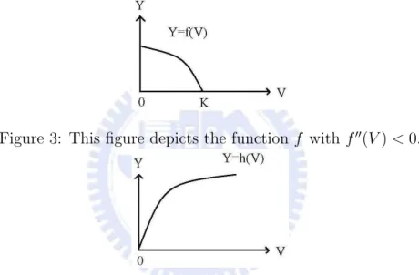
function h(V ) represents the per-capita rate at which predators kill prey; the kill-rate increases as the number of available prey increases, but does so at a decreasing rate, i.e. h(V ) > 0, h0_{(V ) > 0, and h}00_{(V ) < 0. The following Figures 1, 2, 3, 4,}

depict typical graphs for the functions f and h.

In this section, we summarize the propositions obtained in [20], and provide detailed computations for these results.

Figure 1: This figure depicts the function f with f00_{(V ) > 0.}

Figure 2: This figure depicts the function f with f00_{(V ) = 0.}

Figure 3: This figure depicts the function f with f00_{(V ) < 0.}

It is easy to verify that this model has three equilibria, (V, P ) = (0, 0), (K, 0), (J,rJf (J)

kh(J) ).

At first, let us consider these equilibria of the system (3.1). Existence and local stability conditions of these equilibria of the system (3.1) are summarized in propo-sitions 3.1, 3.2.

Proposition 3.1 [20]: Let K be the carrying capacity and J be the equilibrium prey population size. Then

(a) the equilibria (0, 0) and (K, 0) exist for all K; (b) the equilibrium (0, 0) is unstable for all K; (c) the equilibrium (K, 0) is stable for K < J. Proof:

(a) It is easy to see that (0, 0) and (K, 0) exist for all K.

(b) From the system (3.1), we can compute the Jacobian matrix at (V, P ) µ

r[f (V ) + V f0_{(V )] − kP h}0_{(V ) −kh(V )}

AkP h0_{(V ) Ak[h(V ) − h(J)]}

¶

.

Then the Jacobian matrix at the equilibrium (0, 0) is µ

rf (0) −kh(0)

0 Ak[h(0) − h(J)]

¶

.

Hence, its eigenvalues are given by λ=rf (0), Ak[h(0) − h(J)]. Since λ=rf (0) > 0, the equilibrium (0, 0) is unstable for all K.

(c) Similarly, the Jacobian matrix at the equilibrium (K, 0) is µ

r[f (K) + Kf0_{(K)] −kh(K)}

0 Ak[h(K) − h(J)]

¶

.

Therefore, its eigenvalues are given by λ=r[f (K) + Kf0_{(K)], Ak[h(K) − h(J)].}

Both r[f (K)+Kf0_{(K)] and Ak[h(K)−h(J)] are negative for all K < J by hypothesis}

of f and h, the equilibrium (K, 0) is stable for all K < J. The assertion follows. Proposition 3.2 [20]: Let K be the carrying capacity and J be the equilibrium prey population size. Then the equilibrium (J,rJf (J)_kh(J)) exists for for K > J, and is stable

for J < K < Kcrit, where Kcrit is the solution of the equation αf (J) + Jf0(J) = 0,

where α = 1 − Jh_h(J)0(J). In particular, Hopf bifurcation occurs for K = Kcrit.

Proof:

Since f (J) > 0 when J < K, the equilibrium (J,rJf (J)_kh(J) ) exists for for K > J. From the system (3.1), we can compute the Jacobian matrix at (V, P ) is

µ

r[f (V ) + V f0_{(V )] − kP h}0_{(V ) −kh(V )}

AkP h0_{(V ) Ak[h(V ) − h(J)]}

¶

.

Then the Jacobian matrix at the equilibrium (J,rJf (J)_kh(J)) is

M = Ã r[f (J) + Jf0_{(J)] −} rJf (J) h(J) h0(J) −kh(J) AkrJf (J)_kh(J)h0_{(J) 0} ! = Ã r[αf (J) + Jf0_{(J)] −kh(J)} r2_{τ f (J)} kh(J) h0(J) 0 ! , where α = 1 − Jh 0_(J) h(J) , τ = AkJ r h 0_(J).

By Mean Value Theorem, we have h(J)−h(0) = h0_{(c) for some c ∈ (0, J). Moreover,}

h0_{(c) > h}0_{(J) by h}00_{(V ) < 0. Therefore, h(J) > h(J) − h(0) = h}0_{(c)J > h}0_{(J)J, i.e.}

α = 1 −Jh_h(J)0(J) > 0. Since A, k, J, r, h0_{(J) are positive, τ =} AkJ

r h0(J) > 0. In fact,

we have the characteristic equation of M is

λ2 _{− r[αf (J) + Jf}0_{(J)]λ + r}2_{τ f (J) = 0.}

So, its eigenvalues are given by

λ = r[αf (J) + Jf

0_{(J)] ±}p_r2_{[αf (J) + Jf}0_(J)]2_{− 4r}2_{τ f (J)}

2 .

In two dimensional case, we can only use the determinant and the trace to determine the stability of the equilibrium. The determinant and trace of M are r2_{τ f (J) and}

r[αf (J) + Jf0_{(J)], respectively. By Theorem 2, the equilibrium (J,}rJf (J)

kh(J) ) is stable

when the determinant of M is positive and the trace of M is negative, which occurs at

Next, let us compute the derivative of αf (J) + Jf0_{(J) with respect to K.} d[αf (J) + Jf0_(J)] dK = α df (J) dK + J df0_(J) dK > 0.

So, as the control parameter K increases, the equilibrium (J,rJf (J)_kh(J) ) becomes un-stable. Furthermore, we have λ = 0 ±pr2_{τ f (J) and} dRe(λ)

dK 6= 0 when K = Kcrit,

where

αf (J) + Jf0(J) = 0, (3.2) so Hopf bifurcation occurs for K = Kcrit. This completes the proof.

Assume the equilibrium (J,rJf (J)_kh(J) ) is stable, let us compute the eigenvalues of

M and determine the dominant eigenvalue to find the recovery rate. The following

proposition will tell us where the maximum recovery rate occurs. Proposition 3.3 [20]:

Suppose the equilibrium (J,rJf (J)_kh(J)) is stable. Then the maximum recovery rate occurs for some value of K = Kr when δ2 + 4βγ = 0, which occurs at αf (J) +

Jf0_{(J) = −2}p_{τ f (J).}

Proof:

We know that the characteristic equation of the Jacobian matrix at the equilibrium (J,rJf (J)_kh(J) ) is

λ2− r[αf (J) + Jf0(J)]λ + r2τ f (J) = 0

and its eigenvalues are given by

λ = r[αf (J) + Jf 0_{(J)] ±}p_r2_{[αf (J) + Jf}0_(J)]2_{− 4r}2_{τ f (J)} 2 = δ ±pδ2_{+ 4βγ} 2 where β = −kh(J) < 0, γ = r2_kh(J)τ f (J) > 0, δ = r[αf (J) + Jf0_{(J)] < 0.} Let λ+ ≡ δ+ √ δ2_+4βγ 2 , λ− ≡ δ−√δ2_+4βγ

2 . Then we can compute the dominant

eigen-value λdom. First, we divide the situation into two kinds according to δ2+ 4βγ. If

δ2 _{+ 4βγ > 0 then λ} + = δ+ √ δ2_+4βγ 2 > δ−√δ2_+4βγ

2 = λ−. Hence, Re(λ+) > Re(λ−),

i.e. λdom = λ+ = δ+

√

δ2_+4βγ

2 . If δ2 + 4βγ ≤ 0 then Re(λ+) = Re(λ−) =

δ

2, i.e.

λdom = λ+= λ− = δ₂. Thus, the recovery rate ρ ≡ |Re(λdom)| is

(

−δ−√δ2_+4βγ

2 if α2+ 4βγ > 0,

−δ

Finally, let us compute the derivative of ρ with respect to K. Consider α2_{+ 4βγ > 0} and let δ0 ₌ dδ dK Then dρ dK = d(−δ− √ δ2_+4βγ 2 ) dK = −1 2 · d(δ +pδ2_{+ 4βγ)} dK = −δ 0 2 − 1 4pδ2 _{+ 4βγ} · d[δ2_{+ 4(−r}2_{τ f (J))]} dK = −δ0 2 − 1 4pδ2 _{+ 4βγ} · (2δδ 0_{− 4r}2_τdf (J) dK ) = −δ0 2 (1 + δ p δ2_{+ 4βγ}) + r 2_τdf (J) dK > 0 since (1 + _√ δ δ2_+4βγ) < 1 + δ √ δ2 = 1 + δ (−δ) = 0. When α2 + 4βγ < 0, we have dρ dK = d(−δ 2) dK = −r 2 · d[αf (J) + Jf0_(J)] dK < 0

because d[αf (J)+Jf_dK 0(J)] > 0. Therefore, the maximum recovery rate occurs for some

value of K = Kr when δ2+ 4βγ = 0, which occurs when

αf (J) + Jf0_{(J) = −2}p_{τ f (J). (3.3)}

To sum up, if we are using the recovery rate as an indicator of the system (3.1), we will have more warning of the upcoming transition when Kr is far enough

from Kcrit. From equations (3.2) and (3.3), we see that Kr is far away from Kcrit

when the right-hand side of (3.3) tends to minus infinity:

τ f (J) = AkJ r h

0_{(J)f (J) → ∞.}

This occurs as A → ∞ (predator-prey biomass conversion is efficient), r → 0 (the intrinsic rate of increase in the prey population is low), or k → ∞ (predation rate being high). Kr is also far enough from Kcrit when h0(J) → ∞, meaning that

the predation rate increases quickly with increasing prey population size, which is equivalent to the predation rate being high.

4

Three species food chain model

In this section, let us discuss the Lotka-Volterra equation for a food chain of three species [22]. Consider the system of differential equations are given by

dN1 dt = N1(r1− a11N1− a12N2), dN2 dt = N2(r2+ a21N1− a22N2 − a23N3), dN3 dt = N3(r3+ a32N2− a33N3). (4.1) where ri > 0 and aij > 0, ∀ 1 ≤ i, j ≤ 3.

In this model, t is time, Ni is the population of species i, ri is the intrinsic

growth rate of the species i, and aij is the competitive impact of species j on species

i. Moreover, N1 and N2 have a negative effect on the growth rate of N1 ; N1 has a

positive effect and N2 and N3 have a negative effect on the growth rate of N2 ; N2

has a positive effect and N3 have a negative effect on the growth rate of N3. That

is why this model is said to be a food chain.

In order to give a manageable exposition, we henceforth reduce the number of parameters in this three species food chain model by making the symmetry as-sumptions that (i) r1 = r2 = r3 = 1 ; (ii) with respect to species, 2 affects 1 as 3

affects 2, i.e. a12 = a23= α ; (iii) with respect to species, 1 affects 2 as 2 affects 3,

i.e. a21 = a32= β ; (iv) a11= a22 = a33= 1, to arrive at

dN1 dt = N1(1 − N1− αN2), dN2 dt = N2(1 + βN1− N2− αN3), dN3 dt = N3(1 + βN2− N3). (4.2)

The study of equilibria plays a central role in ordinary differential equations and their application. At first, let us find the conditions for existence of the equilib-ria of this system. It can be computed that there exist eight nonnegative equilibequilib-ria for this model:

(i) no-species equilibrium: E0 = (0, 0, 0).

(ii) single species equilibrium: E1 = (1, 0, 0), ˆE1 = (0, 1, 0), ˇE1 = (0, 0, 1).

(iii) two-species equilibrium: E2 = (1, 0, 1), ˆE2 = (0,_1+αβ1−α ,_1+αβ1+β ) , ˇE2 = (_1+αβ1−α ,_1+αβ1+β , 0).

(iv) three species equilibrium: E3 = (1+αβ−α+α

2 1+2αβ , 1+β−α 1+2αβ, 1+αβ+β+β2 1+2αβ ).

Existence conditions of these equilibria of this model are summarized in proposition 4.1.

Proposition 4.1:

(a) E0, E1, ˆE1, ˇE1, and E2 exist and for all values of α, β > 0.

(b) ˆE2 and ˇE2 exist for 0 < α < 1 and β > 0.

(c) E3 exists for α − β < 1.

Proof:

(a) We know that

E0 = (0, 0, 0), E1 = (1, 0, 0), ˆE1 = (0, 1, 0), ˇE1 = (0, 0, 1), E2 = (1, 0, 1). Hence,

no-species equilibrium E0, single species equilibria E1, ˆE1, ˇE1, and two-species

equi-librium E2 exist for all values of α, β > 0.

(b) Since ˆ E2 = (0, 1 − α 1 + αβ, 1 + β 1 + αβ), ˇ

E2 = (_1+αβ1−α ,_1+αβ1+β , 0), two-species equilibria ˆE2, ˇE2 exist for 0 < α < 1 and β > 0.

(c) We know that the three species equilibrium

E3 = ( 1 + αβ − α + α2 1 + 2αβ , 1 + β − α 1 + 2αβ , 1 + αβ + β + β2 1 + 2αβ ),

so there is the three species equilibrium E3when 1+β−α > 0 and 1+αβ−α+α2 > 0.

Since 1 + αβ − α + α2 _{= (α − 1/2)}2_{+ αβ + 3/4 > 0, for all α, β > 0, therefore, the}

three species equilibrium E3 exists for α − β < 1.

It is in general a routine, although often algebraically messy, matter to study the stability of such equilibria. For convenience, at first we only verify the local stability of the equilibria of this system when β = 1. Afterward we focus on stability of the three species equilibrium E3 for various parameters. Local stability conditions

of these equilibria of this model when β = 1 are summarized in proposition 4.2. Proposition 4.2: Let β = 1.

(a) E0, E1, ˆE1, and ˇE1 are unstable for all values of α.

(b) E2 is stable for α > 2 and is unstable for α < 2.

(c) ˆE2 and ˇE2 are unstable for α < 1.

Proof:

First, we compute the Jacobian matrix at (N1, N2, N3)



 1 − 2N_N1₂− αN2 _{1 + N1}−αN_{− 2N}1_{2− αN3 −αN}0 ₂ 0 N3 1 + N2− 2N3

  . Thus, we obtain the Jacobian matrix for each equilibrium of this system. (a) (i) At E0, the Jacobian matrix is



 1 0 0_{0 1 0} 0 0 1

  . Hence, its eigenvalues are given by

λ = 1, 1, 1.

Thus, E0 is always unstable.

(ii) At E1, the Jacobian matrix is



 −1 −α 0_{0 2 0} 0 0 1

  . Therefore, its eigenvalues are given by

λ = −1, 2, 1.

Therefore, E1 is always unstable.

(iii) At ˆE1, the Jacobian matrix is



 1 − α_{1 −1 −α}0 0 0 0 2

  . Thus, its eigenvalues are

λ = 1 − α, −1, 2.

Therefore, ˆE1 is always unstable.

(iv) At ˇE1, the Jacobian matrix is



 1_{0 1 − α}0 0₀ 0 1 −1

  .

So, its eigenvalues are

λ = 1, 1 − α, −1.

Thus , ˇE1 is always unstable.

(b) At E2, the Jacobian matrix is



 −1_{0 2 − α}−α 0₀ 0 1 −1

  .

So, one eigenvalue is positive when α < 2 and all of its eigenvalues are negative when α > 2. Therefore, E2 is stable for α > 2 and is unstable for α < 2.

(c) (i) At ˆE2, the Jacobian matrix is

  1 − α 1−α 1+α 0 0 1−α 1+α 1 − 21−α1+α − α1+α2 −α1−α1+α 0 1−α 1+α 1 + 1−α1+α − 21−α1+α   . So, there is an eigenvalue

λ = 1 − α1 − α

1 + α =

1 + α2

1 + α > 0. Therefore, ˆE2 is unstable for α < 1.

(ii) At ˇE2, the Jacobian matrix is

  1 − 21−α 1+α − α1+α2 −α1−α1+α 0 2 1+α 1 + 1−α1+α − 21+α2 −α1+α2 0 0 1 + 2 1+α   . So, there is an eigenvalue

λ = 1 + 2

1 + α > 0. Therefore, ˇE2 is unstable for α < 1.

(d) At E3, the Jacobian matrix is

  − 1+α2 1+2α 0 0 1−α 1+α −α1+α 2 1+2α −α1+2α2−α 0 3+α 1+2α −1+2α3+α   . So, we can compute its eigenvalues

λ = −1 + α2 1 + 2α, −α α2_{− α + 3} 1 + 2α , − 3 + α 1 + 2α.

Since all of its eigenvalues are negative, E3 is stable for α < 2.

From now on, we concentrate our attention on the stability of the three species equilibrium E3 for various parameters. Here, we introduce an useful method to

de-termine the stability of the three species equilibrium E3 for various parameters. The

method is as follows. Given A ∈ Rn×n_{, Reλ(A) ≡ max{Reλ : λ is an eigenvalue of A}.}

How do we verify analytically A is a stable matrix, i.e. Reλ(A) < 0 ? Suppose that the characteristic polynomial of A is

g(z) = det(zI − A) = a0zn+ a1zn−1+ · · · + an(a0 > 0).

The Routh-Hurwitz Criterion provides a necessary and sufficient condition for a real polynomial to have all roots with negative real parts. We list the conditions for n = 2, 3 which are frequently used in applications.

(i) Assume that n = 2. Then g(z) = a0z2+ a1z + a2 with a1 > 0 and a2 > 0 if

and only if A is a stable matrix.

(ii) Assume that n = 3. Then g(z) = a0z3+ a1z2+ a2z + a3 with a1 > 0, a3 > 0,

and a1a2 > a0a3 if and only if A is a stable matrix.

A more thorough treatment are given in [10, 21].

By Routh-Hurwitz Criterion, we will analyze the stability of the three species equilibrium E3 for various parameters. The result is as follows.

Proposition 4.3: If there exists the three-species equilibrium E3, then E3 is always

an asymptotically stable equilibrium. Proof:

We will apply Routh-Hurwitz Criterion to prove stability of the three-species equi-librium E3. Hence, we desire to acquire the coefficients a0, a1, a2, a3 of the

charac-teristic polynomial of the Jacobian matrix at E3. From the system (4.2), we have

the Jacobian matrix at E3=( ¯N1, ¯N2, ¯N3)

A =   1 − 2 ¯N_{β ¯N}1− α ¯₂ N2 _{1 + β ¯N1}−α ¯_{− 2 ¯}N_N1_{2− α ¯N3 −α ¯}0_N2 0 β ¯N3 1 + β ¯N2− 2 ¯N3   =   − ¯_{β ¯N}N₂1 −α ¯_{− ¯N}N₂1 _{−α ¯}0_N2 0 β ¯N3 − ¯N3   .

Since 1 − 2 ¯N1− α ¯N2 = 1 − 2 · 1 + αβ − α + α2 1 + 2αβ − α · 1 + β − α 1 + 2αβ = −1 + αβ − α + α2 1 + 2αβ = − ¯N1, 1 + β ¯N1− 2 ¯N2− α ¯N3 = 1 + β · 1 + αβ − α + α2 1 + 2αβ − 2 · 1 + β − α 1 + 2αβ − α · 1 + αβ + β + β2 1 + 2αβ = −1 + β − α 1 + 2αβ = − ¯N2, 1 + β ¯N2 − 2 ¯N3 = 1 + β · 1 + β − α 1 + 2αβ − 2 · 1 + αβ + β + β2 1 + 2αβ = −1 + αβ + β + β2 1 + 2αβ = − ¯N3,

So, the characteristic polynomial of the Jacobian matrix at E3 is

det(λI − A) = i=3 Y i=1 (λ + Ni) + αβN1N2(λ + N3) + αβN2N3(λ + N1) = λ3 _{+ ( ¯N} 1+ ¯N2+ ¯N3)λ2+ [(1 + αβ) ¯N1N¯2+ (1 + αβ) ¯N2N¯3+ ¯N3N¯1]λ + (1 + 2αβ) ¯N1N¯2N¯3.

It is easy to see the coefficients a0, a1, a2, a3 of the characteristic polynomial of the

Jacobian matrix at E3 are

a0 = 1,

a1 = ¯N1+ ¯N2+ ¯N3 > 0,

a2 = (1 + αβ) ¯N1N¯2+ (1 + αβ) ¯N2N¯3+ ¯N3N¯1,

Therefore, we have a1a2− a0a3 = ( ¯N1 + ¯N2+ ¯N3)[(1 + αβ) ¯N1N¯2+ (1 + αβ) ¯N2N¯3+ ¯N3N¯1] − (1 + 2αβ) ¯N1N¯2N¯3 = ¯N12( ¯N2+ ¯N3) + ¯N2( ¯N3+ ¯N1) + ¯N32( ¯N1+ ¯N2) + 3 ¯N1N¯2N¯3+ 2αβ ¯N1N¯2N¯3 + αβ( ¯N12N¯2+ ¯N1N¯22+ ¯N22N¯3+ ¯N2N¯32) − ¯N1N¯2N¯3− 2αβ ¯N1N¯2N¯3 = ¯N12( ¯N2+ ¯N3) + ¯N22( ¯N3+ ¯N1) + ¯N32( ¯N1+ ¯N2) + 2 ¯N1N¯2N¯3 + αβ( ¯N12N¯2+ ¯N1N¯22+ ¯N22N¯3+ ¯N2N¯32) > 0.

By Routh-Hurwitz Criterion, the assertion follows.

Next, we perform some numerical simulations for various α, β, to explore global dynamics for the system. The numerical computations provide us some observation and motivation to justify more dynamical properties for the three-species equilibrium

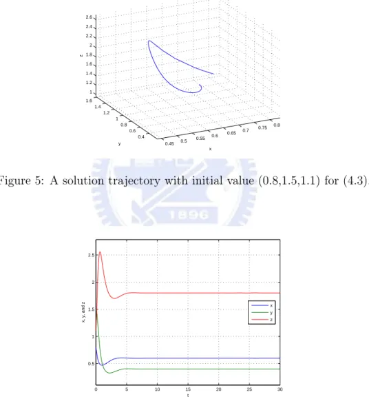
Example 4.1: If α = 1 and β = 2, i.e., the system is dN1 dt = N1(1 − N1− N2) dN2 dt = N2(1 + 2N1− N2 − N3) dN3 dt = N3(1 + 2N2− N3) (4.3)

then E3=(3₅,2₅,9₅) is an asymptotically stable equilibrium for the above system. (See

Figure 5, Figure 6.) 0.45 0.5 0.55 0.6 0.65 0.7 0.75 0.8 0.4 0.6 0.8 1 1.2 1.4 1.6 1 1.2 1.4 1.6 1.8 2 2.2 2.4 2.6 x y z

Figure 5: A solution trajectory with initial value (0.8,1.5,1.1) for (4.3).

0 5 10 15 20 25 30 0.5 1 1.5 2 2.5 t x, y, and z x y z

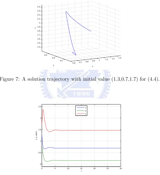
Example 4.2: If α = 2 and β = 3, i.e., the system is dN1 dt = N1(1 − N1 − 2N2) dN2 dt = N2(1 + 3N1− N2− 2N3) dN3 dt = N3(1 + 3N2− N3) (4.4)

then E3=(₁₃9 ,₁₃2,19₁₃) is an asymptotically stable equilibrium for the above system.

(See Figure 7, Figure 8.)

0.6 0.7 0.8 0.9 1 1.1 1.2 1.3 0.2 0.4 0.6 1.4 1.5 1.6 1.7 1.8 1.9 2 2.1 2.2 2.3 2.4 x y z

Figure 7: A solution trajectory with initial value (1.3,0.7,1.7) for (4.4).

0 5 10 15 20 25 30 0 0.5 1 1.5 2 2.5 t x, y, and z x y z

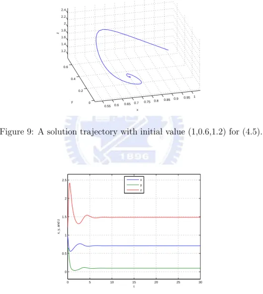
Example 4.3: If α = 3 and β = 5, i.e., the system is dN1 dt = N1(1 − N1 − 3N2) dN2 dt = N2(1 + 5N1− N2− 3N3) dN3 dt = N3(1 + 5N2− N3) (4.5)

then E3=(22₃₁,₃₁3,46₃₁) is an asymptotically stable equilibrium for the above system.

(See Figure 9, Figure 10.)

0.55 0.6 0.65 0.7 0.75 0.8 0.85 0.9 0.95 1 0 0.2 0.4 0.6 1.2 1.4 1.6 1.8 2 2.2 2.4 x y z

Figure 9: A solution trajectory with initial value (1,0.6,1.2) for (4.5).

0 5 10 15 20 25 30 0 0.5 1 1.5 2 2.5 t x, y, and z x y z

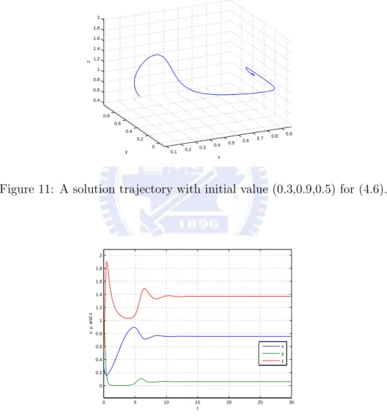
Example 4.4: If α = 4 and β = 6, i.e., the system is dN1 dt = N1(1 − N1 − 4N2) dN2 dt = N2(1 + 6N1− N2− 4N3) dN3 dt = N3(1 + 6N2− N3) (4.6)

then E3=(37₄₉,₄₉3,67₄₉) is an asymptotically stable equilibrium for the above system.

(See Figure 11, Figure 12.)

0.1 0.2 0.3 0.4 0.5 0.6 0.7 0.8 0.9 0 0.2 0.4 0.6 0.8 0.4 0.6 0.8 1 1.2 1.4 1.6 1.8 2 x y z

Figure 11: A solution trajectory with initial value (0.3,0.9,0.5) for (4.6).

0 5 10 15 20 25 30 0 0.2 0.4 0.6 0.8 1 1.2 1.4 1.6 1.8 2 t x, y, and z x y z

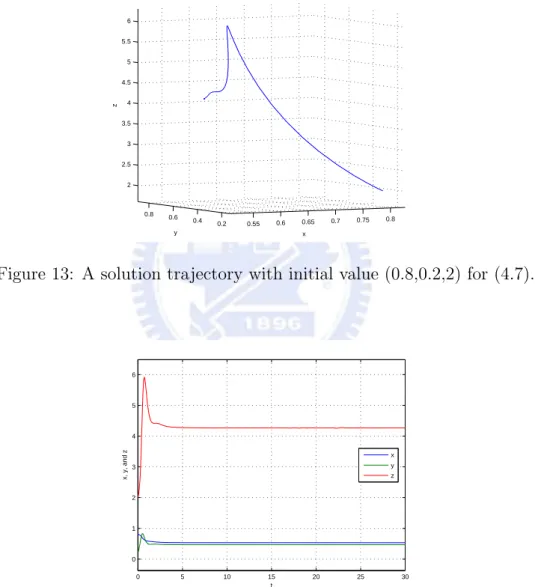
Example 4.5: If α = 1 and β = 7, i.e., the system is dN1 dt = N1(1 − N1− N2) dN2 dt = N2(1 + 7N1− N2 − N3) dN3 dt = N3(1 + 7N2− N3) (4.7)

then E3=(₁₅8 ,₁₅7,64₁₅) is an asymptotically stable equilibrium for the above system.

(See Figure 13, Figure 14.)

0.55 0.6 0.65 0.7 0.75 0.8 0.2 0.4 0.6 0.8 2 2.5 3 3.5 4 4.5 5 5.5 6 x y z

Figure 13: A solution trajectory with initial value (0.8,0.2,2) for (4.7).

0 5 10 15 20 25 30 0 1 2 3 4 5 6 t x, y, and z x y z

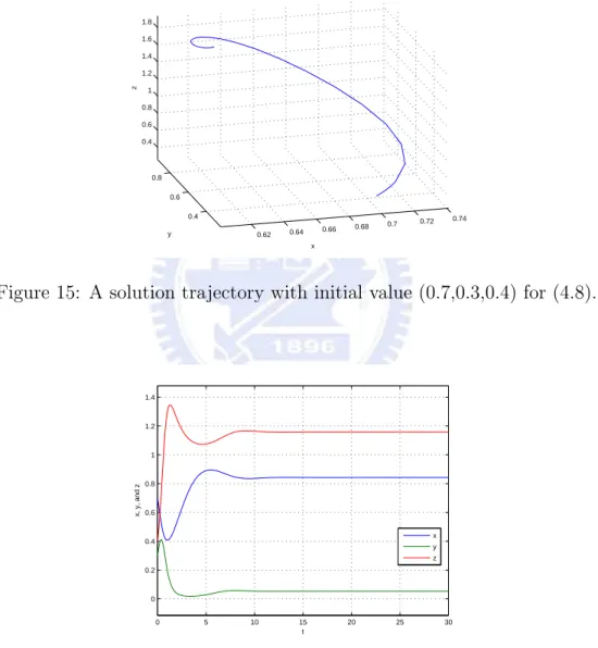
Example 4.6: If α = 0.5 and β = 1, i.e., the system is dN1 dt = N1(1 − N1− 0.5N2) dN2 dt = N2(1 + N1− N2− 0.5N3) dN3 dt = N3(1 + N2− N3) (4.8)

then E3=(5₈,3₄,7₄) is an asymptotically stable equilibrium for the above system. (See

Figure 15, Figure 16.) 0.62 0.64 0.66 0.68 0.7 0.72 0.74 0.4 0.6 0.8 0.4 0.6 0.8 1 1.2 1.4 1.6 1.8 x y z

Figure 15: A solution trajectory with initial value (0.7,0.3,0.4) for (4.8).

0 5 10 15 20 25 30 0 0.2 0.4 0.6 0.8 1 1.2 1.4 t x, y, and z x y z

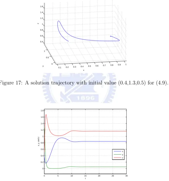
Example 4.7: If α = 3 and β = 3, i.e., the system is dN1 dt = N1(1 − N1 − 3N2) dN2 dt = N2(1 + 3N1− N2− 3N3) dN3 dt = N3(1 + 3N2− N3) (4.9)

then E3=(16₁₉,₁₉1,22₁₉) is an asymptotically stable equilibrium for the above system.

(See Figure 17, Figure 18.)

0.1 0.2 0.3 0.4 0.5 0.6 0.7 0.8 0.9 1 0 0.5 1 0.4 0.6 0.8 1 1.2 1.4 1.6 x y z

Figure 17: A solution trajectory with initial value (0.4,1.3,0.5) for (4.9).

0 5 10 15 20 25 30 0 0.2 0.4 0.6 0.8 1 1.2 1.4 1.6 1.8 t x, y, and z x y z

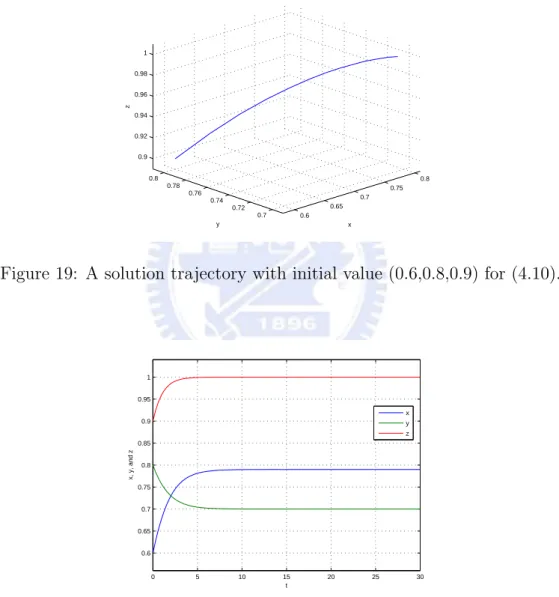
Example 4.8: If α = 0.3 and β = 0.00000000000000001, i.e., the system is dN1 dt = N1(1 − N1− 0.3N2) dN2 dt = N2(1 + 0.00000000000000001N1− N2− 0.3N3) dN3 dt = N3(1 + 0.00000000000000001N2− N3) (4.10)

then E3 ≈ (0.79, 0.7, 1) is an asymptotically stable equilibrium for the above system.

(See Figure 19, Figure 20.)

0.6 0.65 0.7 0.75 0.8 0.7 0.72 0.74 0.76 0.78 0.8 0.9 0.92 0.94 0.96 0.98 1 x y z

Figure 19: A solution trajectory with initial value (0.6,0.8,0.9) for (4.10).

0 5 10 15 20 25 30 0.6 0.65 0.7 0.75 0.8 0.85 0.9 0.95 1 t x, y, and z x y z

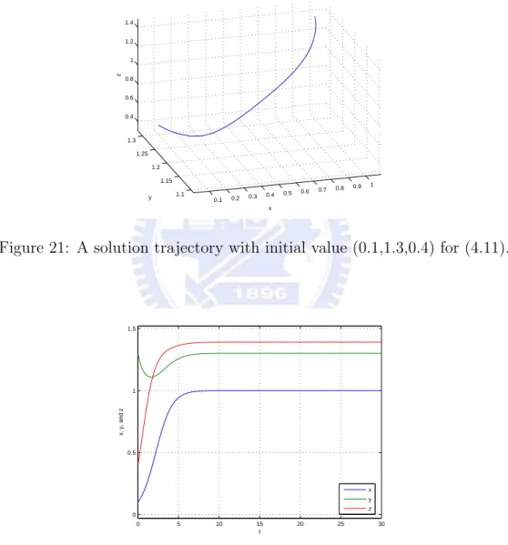
Example 4.9: If α = 0.00000000000000001 and β = 0.3, i.e., the system is dN1 dt = N1(1 − N1− 0.00000000000000001N2) dN2 dt = N2(1 + 0.3N1− N2− 0.00000000000000001N3) dN3 dt = N3(1 + 0.3N2− N3) (4.11)

then E3 ≈ (1, 1.3, 1.39) is an asymptotically stable equilibrium for the above system

(see Figure 21, Figure 22.)

0.1 0.2 0.3 0.4 0.5 0.6 0.7 0.8 0.9 1 1.1 1.15 1.2 1.25 1.3 0.4 0.6 0.8 1 1.2 1.4 x y z

Figure 21: A solution trajectory with initial value (0.1,1.3,0.4) for (4.11).

0 5 10 15 20 25 30 0 0.5 1 1.5 t x, y, and z x y z

According to above proposition and examples, we might apparently observe that the three-species equilibrium is not only asymptotically stable but also globally attracting when it exists. The following result states this more precisely.

Theorem 4.1: Assume there is an equilibrium (p1, p2, p3) for the three-species

food chain model (4.1) with pi > 0, i = 1, 2, 3. Then the basin of attraction of the

equilibrium (p1, p2, p3) includes the first octant {(N1, N2, N3) : N1 > 0, N2 > 0, N3 >

0}. Proof:

Suppose there is an equilibrium (p1, p2, p3) for three species food chain model with

pi > 0, i = 1, 2, 3. Then    p1(r1− a11p1− a12p2) = 0 p2(r2+ a21p1− a22p2− a23p3) = 0 p3(r3+ a32p2− a33p3) = 0 ⇒    r1 = a11p1+ a12p2 r2 = −a21p1+ a22p2+ a23p3 r3 = −a32p2+ a33p3 Let x1 = r1− a11N1− a12N2, x2 = r2+ a21N1− a22N2− a23N3, and x3 = r3+ a32N2− a33N3. Then, we set x1 := (a11p1+ a12p2) − a11N1− a12N2 = a11(p1− N1) + a12(p2− N2), x2 := (−a21p1+ a22p2+ a23p3) + a21N1− a22N2− a23N3 = −a21(p1− N1) + a22(p2− N2) + a23(p3− N3), x3 := (−a32p2+ a33p3) + a32N2 − a33N3 = −a32(p2− N2) + a33(p3− N3).

Now, we define a function L by

L(N1, N2, N3) = c1[N1− p1ln (N1)] + c2[N2− p2ln (N2)] + c3[N3− p3ln (N3)] = 3 X i=1 ci[Ni − piln (Ni)], where c2 c1 = a12 a21, c3 c2 = a23

a32 and cij > 0, for i = 1, 2, 3. Then L(N1, N2, N3) >

and ˙L(N1, N2, N3) = c1(1 − p1· 1 N1 ) · N1x1+ c2(1 − p2· 1 N2 ) · N2x2+ c3(1 − p3· 1 N3 ) · N3x3 = c1(N1− p1)x1 + c2(N2− p2)x2 + c3(N3− p3)x3 = c1(N1− p1)[a11(p1− N1) + a12(p2− N2)] + c2(N2− p2)[−a21(p1− N1) + a22(p2− N2) + a23(p3− N3)] + c3(N3− p3)[−a32(p2− N2) + a33(p3− N3)] = −a11c1(N1− p1)2− a22c2(N2− p2)2− a33c3(N3− p3)2 + (−a12c1+ a21c2)(N1− p1)(N2− p2) + (−a23c2+ a32c3)(N2− p2)(N3− p3). Since c2 c1 = a12 a21 and c3 c2 = a23

a32, −a12c1 + a21c2 = −a23c2+ a32c3 = 0, then

˙L(N1, N2, N3) = −a11c1(N1− p1)2− a22c2(N2− p2)2− a33c3(N3− p3)2 = − 3 X i=1 aiici(Ni− pi)2.

i.e. for all (N1, N2, N3) 6= (p1, p2, p3), ˙L(N1, N2, N3) < 0 and ˙L(p1, p2, p3) = 0.

Therefore, L is a Lyapunov function on {(N1, N2, N3) : N1 > 0, N2 > 0, N3 > 0}. By

Theorem 2.4, the assertion holds.

Finally, let us compute the recovery rate at the stable equilibria E2 = (1, 0, 1)

and E3 = (1+αβ−α+α 2 1+2αβ , 1+β−α 1+2αβ, 1+αβ+β+β2

1+2αβ ), respectively. For arithmetical convenience,

we only compute the recovery rate of the stable equilibria E2, E3 when β = 1. Of

course, we can use similar method to calculate the recovery rate at the stable equi-librium E3 for the other case. For β = 1, the recovery rate at the stable equilibria

E2, E3 are summarized in proposition 4.4.

Proposition 4.4: Let β = 1. Assume that E2 and E3 are stable equilibria. Let α0

be the solution of the equation α3_{− 2α}2_{+ 3α − 1 = 0.}

(a) The recovery rate at the stable equilibrium E2 is α − 2 when 2 < α < 3. It means

the recovery rate at the stable equilibrium E2 is increasing with respect to α.

(b) The recovery rate at the stable equilibrium E2 is 1 when α ≥ 3. It means the

(c) The recovery rate at the stable equilibrium E3 is 3α−α

2_+α3

1+2α when 0 < α < α0.

(d) The recovery rate at the stable equilibrium E3 is 1+α

2

1+2α when α0 < α < 2.

Proof:

(a)(b)Let β = 1. By Proposition 4.1, 4.2, we have E2 = (1, 0, 1) exists and is stable

when α > 2. At E2, the Jacobian matrix is



 −1_{0 2 − α}−α 0₀ 0 1 −1

 

and its eigenvalues are λ = −1, 2 − α, −1. So, the dominant eigenvalue λdom at E2 is

½

2 − α if 2 < α < 3,

−1 if α ≥ 3. Therefore, the recovery rate ρ ≡ |Re(λdom)| at E2 is

½

α − 2 if 2 < α < 3,

1 if α ≥ 3. (c)(d) Similarly, E3 = (1+α

2

1+2α,1+2α2−α ,1+2α3+α) exists and is stable when α < 2. At E3, the

Jacobian matrix is   − 1+α2 1+2α 0 0 1−α 1+α −α1+α 2 1+2α −α1+2α2−α 0 3+α 1+2α −1+2α3+α   and its eigenvalues are

λ = −1 + α 2 1 + 2α, − 3α − α2_{+ α}3 1 + 2α , − 3 + α 1 + 2α.

Since (i) 1 + α2 _{< 3 + α for 0 < α < 2; (ii) 3α − α}2 _{+ α}3 _{< 1 + α}2 _{for 0 < α < α} 0;

(iii) 3α − α2_{+ α}3 _{> 1 + α}2 _{for α}

0 < α < 2, where α0 is the solution of the equation

α3 _{− α}2 _{+ 3α − 1 = 0. By Maple, we can compute α}

0 ≈ 0.4301597088. So, the

dominant eigenvalue λdom at E3 is

(

−3α−α2_+α3

1+2α if 0 < α < α0,

−1+α2

1+2α if α0 < α < 2.

Therefore, the recovery rate ρ ≡ |Re(λdom)| at E3 is

(

3α−α2_+α3

1+2α if 0 < α < α0, 1+α2

1+2α if α0 < α < 2.

5

Genetic control system

In this section, we mention a basic model in genetic control system. The following system has been discussed by [16] as a model for a genetic control system. The activity of a certain gene is assumed to be directly induced by two copies of the protein for which it codes. In other words, the gene is stimulated by its own product, potentially leading to an autocatalytic feedback process. In dimensionless form, the equations are dx dt = −ax + y dy dt = x2 1 + x2 − by (5.1) where x and y are proportional to the concentrations of the protein and messenger RNA from which it is translated, respectively, and a, b > 0 are parameters that govern the rate of degradation of x and y.

First, we shall prove a simple result toward the system (5.1). The result is as follows. It can be proved from Bendixson’s Negative Criterion.

Proposition 5.1: There does not exist periodic solution in the first quadrant

{(x, y) : x > 0, y > 0} for the system (5.1).

Proof:

On {(x, y) : x > 0, y > 0}, the divergence of the vector field is

∂

∂x(−ax + y) + ∂ ∂y(

x2

1 + x2 − by) = −a − b = −(a + b) < 0.

By Theorem 2.5, the assertion holds.

Next, we will show that the system (5.1) has three equilibria when a < acrit,

where acrit is to be determined. Moreover, two of these equilibria coalesce in a

saddle-node bifurcation when a = acrit. Then we will sketch the phase portrait

for a < acrit, and give a biological interpretation. These results are summarized in

proposition 5.2, 5.3.

Proposition 5.2 [15]: The system (5.1) has three equilibria when a < acrit, where

acrit = 1/2b. In particular, two of these equilibria coalesce in a saddle-node

Proof:

One of the most useful tools for analyzing nonlinear systems of differential equa-tions (especially planar systems) are nullclines. If we determine all of the null-clines of the system (5.1), then the intersections of the x- and y-nullnull-clines yields the equilibria. From the system (5.1), we have the nullclines are given by the line y = ax and y = x2

b(1+x2₎. To find acrit, we compute the equilibria directly

and find where they coalesce. Since the nullclines intersect when ax = x2

b(1+x2₎,

the equilibrium (0, 0) always exists for any parameters a, b > 0 and there are equi-libria (x∗_{, y}∗₎₌₍1+√1−4a2_b2 2ab ,1+ √ 1−4a2_b2 2b ), (1− √ 1−4a2_b2 2ab ,1− √ 1−4a2_b2 2b ) if 1 − 4a2b2 > 0, i.e.

ab < 1/2. So, these two equilibria coalesce when ab = 1/2 and therefore acrit = 1/2b.

The assertion follows.

The nullclines also provide a lot of information about the phase portrait for

a < acrit. The vector field is vertical on the line y = ax and horizontal on the curve

y = x2

b(1+x2₎. It appears that the equilibrium (1−

√

1−4a2_b2

2ab ,

1−√1−4a2_b2

2b ) is a saddle and

the other two are sinks. To confirm this, we turn to classify these equilibria.

Proposition 5.3 [15]: If the system (5.1) has three equilibria, i.e. a < acrit then the

equilibria (0, 0) and (1+√1−4a2_b2

2ab ,

1+√1−4a2_b2

2b ) are stable and (

1−√1−4a2_b2 2ab , 1−√1−4a2_b2 2b ) is unstable. Proof:

From the system (5.1), we find the Jacobian matrix at (x, y) is

A = µ −a 1 2x (1+x2₎2 −b ¶ .

A has trace τ = −(a + b) < 0, so all equilibria are either sinks or saddles by

theorem 2.2. At (0, 0), the determinant ∆ = ab > 0, so the origin is always a stable equilibrium. In fact, it is a stable node, since τ2_{− 4∆ = (a − b)}2 _{> 0 (except in the}

degenerate case a = b). For the other two fixed points, we can compute that ∆ = ab − 2x [1 + (x)2_]2 = ab[1 − 2 1 + (x)2] = ab[ −1 + (x)2 1 + (x)2 ]. At (1−√1−4a2_b2 2ab ,1− √ 1−4a2_b2

2b ), the determinant ∆ < 0 since 0 < 1−

√

1−4a2_b2

2ab < 1. Hence,

we have the equilibrium (1−√1−4a2_b2

2ab ,1− √ 1−4a2_b2 2b ) is a saddle. At (1+ √ 1−4a2_b2 2ab ,1+ √ 1−4a2_b2 2b ), the determinant ∆ = ab − 2x [1+(x)2_]2 = ab[1 − _1+(x)2 2] < ab since 1+ √ 1−4a2_b2 2ab > 1. So,

τ2 _{− 4∆ = (a + b)}2_{− 4ab −} 2x

[1+(x)2_]2 = (a − b)2 +_[1+(x)8x2_]2 > (a − b)2 > 0. Thus, the

equilibrium (1+√1−4a2_b2

2ab ,

1+√1−4a2_b2

2b ) is a stable node. This completes the proof.

The phase portrait and the nullclines for the system (5.1) when a = 0.92 and

b = 0.5 are plotted in Figure 23. And we plot the bifurcation diagram for (5.1) when b = 0.5 in Figure 24.

Figure 23: The phase portrait and the nullclines for the system (5.1) when a = 0.92 and b = 0.5. 0 0.2 0.4 0.6 0.8 1 1.2 1.4 1.6 1.8 2 0 1 2 3 4 5 0 0.5 1 1.5 2 2.5 3 3.5 4 4.5 5 a LP LP BP BP H H x y

More importantly, the stable manifold separates the plane into two regions, each a basin of attraction for a sink. The biological interpretation is that the system can act like a biochemical switch, but only if the mRNA and protein degrade slowly enough-specifically, their decay rates must satisfy ab < 1/2. In this case, there are two stable steady states: one at the origin, meaning that the gene is silent and there is no protein around to turn it on; and one where x and y are large, i.e. (x, y) = (1+√1−4a2_b2

2ab ,1+

√

1−4a2_b2

2b ), meaning that the gene is active and sustained by

the high level of protein. The stable manifold of the saddle acts like a threshold; it determines whether the gene turns on or off, depending on the initial values of x and y. Finally, let us compute the recovery rate at the stable equilibrium (1+√1−4a2_b2

2ab ,

1+√1−4a2_b2

2b ). For arithmetical convenience we only investigate for b =

1/2. Of course, we can use similar method to calculate the recovery rate at the stable equilibrium (1+√1−4a2_b2

2ab ,

1+√1−4a2_b2

2b ) for the other case. When b = 1/2, the

characteristic equation of A is

λ2_{+ (a + 1/2)λ +} a

2(

−1 + x2

1 + x2 ) = 0.

So, its eigenvalues are given by

λ = −(a + 1 2) ± q (a + 1 2)2− 2a[ −a2₊₍₁₊√_1−a2₎2 a2₊₍₁₊√_1−a2₎2 ] 2 .

Therefore, the dominant eigenvalue

λdom= −(a +1 2) + q (a +1 2)2− 2a[ −a2₊₍₁₊√_1−a2₎2 a2₊₍₁₊√_1−a2₎2 ] 2 .

At the stable equilibrium (1+√1−4a2_b2

2ab ,

1+√1−4a2_b2

2b ), the recovery rate

ρ ≡ |Re(λdom)| = (a +1 2) − q (a +1 2)2− 2a[ −a2₊₍₁₊√_1−a2₎2 a2₊₍₁₊√_1−a2₎2 ] 2 . Let f0_{(a) = (a +} 1 2) − q (a +1 2)2− 2a[ −a2₊₍₁₊√_1−a2₎2

a2₊₍₁₊√_1−a2₎2 ]. By Matlab, we calculate

f0_{(a) = 0 only when a = a}

r ≈ 0.4676, f0(a) > 0 when a < ar, and f0(a) < 0

when a > ar. Then f has a local maximum at a = ar ≈ 0.4676. Therefore, the

maximum recovery rate occurs for a = ar ≈ 0.4676. To sum up, if we are using

the recovery rate as an indicator of the system (5.1), we will have more warning of the upcoming transition when ar is far enough from acrit. So far, we have seen that

acrit = 1 and ar ≈ 0.4676 when b = 1/2, it will help us judge the dynamics of the

References

[1] Hale, J. K., 1980, Ordinary Differential Equations, Malabar, Florida: Robert E. Krieger.

[2] Robinson, C., An introduction to dynamical systems: Continuous and Discrete, 2004, Pearson.

[3] Holling, C. S., 1973, Resilience and stability of ecological systems, Annual Review of Ecology and Systematics 4: 1-23.

[4] Wissel, C., 1984. A universal law of the characteristic return time near

thresh-olds, Oecologia 65: 101-107.

[5] van Nes, E. H., Scheffer, M., 2007, Slow recovery from perturbations as a generic

indicator of a nearby catastrophic shift, American Naturalist 169: 738-747.

[6] van Nes, E. H., Scheffer, M., 2004, Large species shifts triggered by small forces, American Naturalist 164 : 255-266.

[7] Scheffer, M., Carpenter, S. R., 2003, Catastrophic regime shifts in ecosystems:

linking theory to observation, Trends in Ecology and Evolution 18: 648-656.

[8] Robinson, C., 1995, Dynamical Systems: Stability Symbolic Dynamics, and

Chaos, CRC Press, Boca Raton London New York Washington, D.C.

[9] Jordan, D. W., and Smith, P., 1999, Nonlinear Ordinary Differential Equations,

3rd Edition, Oxford University Press.

[10] Hsu, S. B., 2006, Ordinary differential equations with applications, World Sci-entific Publishing Company.

[11] Wiggins, S., 1990, Introduction to Applied Nonlinear Dynamical Systems and

Chaos, Springer-Verlag.

[12] Kostelich, E. J., and Armbruster, D., 1997, Introductory Differential Equations:

From Linearity to Chaos, Addison-Wesley.

[13] Perko, L., 2000, Differential Equations and Dynamical Systems, Springer-Verlag.

[14] Hirsch, M. W., Smale, S., and Devaney, R. L., 2004. Differential Equations,

Dynamical Systems, and An Introduction to Chaos, 2rd Edition, Academic Press.

[15] Strogatz, S. H., 1994, Nonlinear dynamics and chaos: with applications to

physics, biology, chemistry, and engineering, Addison-Wesley.

[16] Griffith, J. S., 1971, Mathematical Neurobiology, Academic Press.

[17] Pimm, S. L., 1984, The complexity and stability of ecosystems, Nature 307: 321-326.

[18] DeAngelis, D. L.,1980, Energy-flow, nutrient cycling and ecosystem resilience, Ecology 61: 764-771.

[19] Nakajima, H., DeAngelis, D. L., 1989, Resilience and local stability in a

nutrient-limited consumer system, Bulletin of Mathematical Biology 51:

501-510.

[20] Chisholm, R. A., Filotas, E., 2009, Critical slowing down as an indicator of

transitions in two-species models, Journal of Theoretical Biology 257: 142-149.

[21] Coppel, W. A., 1965, Stability and asymptotic behavior of differential equations, Heath, Boston.

[22] Krikorian, N., 1979, The Volterra Model for Three Species Predator-Prey