時空正交分頻多工調變之盲式通道估計

國 立 交 通 大 學

電信工程學系碩士班

碩士論文

時空正交分頻多工調變之盲式通道估計

Blind Channel Estimation for

Space-Time OFDM

研 究 生： 吳泰云

時空正交分頻多工調變之盲式通道估計

Blind Channel Estimation for

Space-Time OFDM

研 究 生：吳泰云 Student：T. Y. Wu

指導教授：謝世福 博士 Advisor：Dr. S.F. Hsieh

國立交通大學

電信工程學系碩士班

碩士論文

A Thesis

Submitted to Department of Communication Engineering

College of Electrical Engineering and Computer Science

National Chiao Tung University

In Partial Fulfillment of the Requirements

For the Degree of

Master of Science

In

Electrical Engineering

July, 2004

Hsinchu, Taiwan, Republic of China

時空正交分頻多工調變

之盲式通道估計

學生：吳泰云 指導教授：謝世福

國立交通大學電信工程學系碩士班

摘要

時空正交分頻多工調變不僅可以達到高傳輸效率而且可以利用分集增益

(diversity gain)，所以目前倍受矚目。在本篇論文中，我們採用了 Giannakis

所提出的時空正交分頻多工調變之盲式通道估計，並且為此估計子推導出均方誤

差。不僅如此，我們更介紹了 decision direct (DD) 和 phase direct (PD) 兩 個方法來使之前所提的通道估計更加趨於理想。 DD 是利用解得的決策信號來更 新通道的估測，而 PD 是在我們得到通道的振幅響應之後，解得其相角響應，原 來是只應用在一般的正交分頻多工上， 因為其通道的振幅響應很容易得到，但 是在時空正交分頻多工調變上，因為接收到的信號是由兩個傳送天線傳來的，通 道的振幅響應很難由其中解出。所以我們提出了一和差平方的演算法來的到通道

Blind Channel Estimation for

Space-Time OFDM

Student: T. Y. Wu Advisor: S. F. Hseieh

Department of Communication Engineering

National Chiao Tung University

Abstract

Space time (ST) orthogonal frequency division multiplexing (OFDM) has been well documented as an attractive means of achieving high data rate transmissions with diversity gains. In this thesis, we adopt a blind channel estimation algorithm proposed by Giannakis for ST OFDM, and derive the theoretical mean square error of the estimator. Moreover, we introduce phase direct (PD) and decision direct (DD) methods to further improve the performance of the estimator. DD and PD originally work on conventional OFDM, and PD is not suited for ST OFDM. Then we derive a new algorithm named sum-difference square method to make PD work on ST OFDM. DD is to update our estimated channel from the previous hard decision data, while PD is to solve the phase ambiguities after we’ve got the channel power response. Since the received data in ST OFDM is composed of two different transmitted data, the channel amplitude response is not easy to get. Hence, the aforementioned algorithm is about how to solve this problem. Furthermore, in computer simulations, we can see our algorithm really better the performance.

Acknowledgement

I would like to express my deepest gratitude to Dr. S. F. Hsieh for his enthusiastic guidance and great patient. I also wish to thank my friends for their concern and help. Finally, I would like to thank my parents, family about their consideration and encouragement.

Contents

1 Introduction

...1

2 Space Time OFDM System Mode l

… … … 5

3 Blind Channel Estimation

… ...13

3.1 Subspace-based multichannel estimation… … … .… … . 13

3.1.1 Noise free case… … … … ...… … … ..13

3.1.1 Noisy case… … … 16

3.2 Performance analysis… … … .17

4

Improved Subspace Methods

… … … ..24

4.1 Decision direct (DD)… … … 25

4.1.1 DD in ST-OFDM… … … 25

4.1.2 Comparison with conventional OFDM … … … ..30

4.2 Phase direct (PD)… … … ..31

4.2.2 PD in ST-OFDM based on sum-difference square algorithm… … … … .34

4.2.3 Choice of window size… … … 37

4.2.4 Precoder design… … … ...40

5 Computer Simulations

… … … 42

5.1 Subspace-based method… … … ...… 42

5.1.1 Estimator error v.s. SNR … … … 43

5.1.2 Estimator error v.s. data block length … … … .44

5.2 Performance of PD and DD … … … ...46

5.3 Time-varying channel estimation… … … … 50

5.3.1 Subspace-based method… … … ..50

5.3.2 Performance of DD and PD… … … .53

List of Figures

2.1 Block precoded ST-OFDM transceiver model … … … 6

2.2 Frequency domain version of Fig. 2.1… … … ...… … ....9

4.1 Signal- flow graph of DD in space-time OFDM… … … ..29

4.2 Signal- flow graph of DD in space-time OFDM… … … ..31

4.3 Signal- flow graph of phase direct in conventional OFDM… … … .34

4.4 Signal- flow graph of finding 2 2 1( m) and 2( m) H ρ H ρ … … … ...37

4.5 Signal- flow graph of phase direct on space-time OFDM in static channel… … .39

4.6 Signal- flow graph of phase direct on space-time OFDM in time varying channel… … … ...… ...40

4.7 Forms of precoder… … … ..… … … ...41

5.1 Channel error of simulation result and theory V.S SNR… … … ...… ...… ..44

5.2 Channel error of simulation result and theory V.S. received data block… … ...45

5.3 Channel error of different multipath length… … … .… … … .46

5.4 Channel error of PD and DD with denoising and without denoising… … … … 47

5.5 PD and DD v.s subspace-based estimator… … … .48

5.6 Testing DD and PD initialized with subspace method for different multipath length… … … ..49

5.7 Testing DD in different data constellation … … … ...50

5.8 Testing of the subspace-based channel estimator in different Doppler frequencies for received blocks equaling to 100… … … ..51

5.9 Testing of the subspace-based channe l estimator in different Doppler frequencies for received blocks equaling to 50 … … … .… 52

5.10 Channel error for each block… … … ...53 5.11 Test of DD and PD in fd=100Hz… … … .54 5.12 Test of DD for different data constellation in fd=50… … … ...55

Chapter 1

Introduction

In orthogonal frequency division multiplexing (OFDM) [1,2,3], the entire channel is divided into many narrow parallel subchannels, thereby increasing the symbol duration and reducing or eliminating the intersymbol interference (ISI) caused by the multipath environments. On the other hand, since the dispersive property of wireless channels causes frequency selective fading, there is higher error probability for those subchannels in deep fades. Hence, techniques such as error correction code and diversity have to be used to compensate for the frequency selectivity. In this thesis, we investigate transmitter diversity using space-time coding for OFDM systems.

Space-time codes (STC) [4,5,6,7] realize the diversity gains by introducing temporal and spatial correlation into the signals transmitted from different antennas without increasing the total transmitted power or transmission bandwidth. There is in fact a diversity gain that results from multiple paths between base station and user terminal, and a coding gain that results from how symbols are correlated across transmit antennas.

Transmitter diversity is an effective technique for combating fading in mobile wireless communications, especially when receiver diversity is expensive or impractical. Many researchers [8,9,10] have studied transmitter diversity for wireless systems. In this thesis, we focus on two transmit-antennas and one receive-antenna and use the well known Alamouti’s block STC [11].

However, for most STC transceivers, multichannel estimation algorithms are needed. Training symbols are transmitted periodically in [12] for the receiver to acquire the multi- input multi-output (MIMO) frequency- flat channels (see also [13] for training-based estimation of frequency-selective channels in ST-OFDM). However, training sequences consume bandwidth and, thereby, incur spectral efficiency (and thus capacity) loss. For this reason, blind channel estimation methods receive growing attention, especially for estimating the MIMO channels corresponding to multiple transmit and receive antennas.

Only a few works, however, have been reported so far on blind MIMO and multi- input single-output (MISO) channel estimation that exploits the unique features of ST codes. Relying on nonredundant and nonconstant modulus precoding, blind channel estimation and equalization for OFDM-based multi-antenna systems has been proposed in [14] using cyclostationary statistics. Subspace-based blind method is proposed in [15] for estimating the channel responses of a multiuser and multiantenna OFDM uplink system. For ST-OFDM, a deterministic blind channel estimator was derived in [16] when the channel transfer functions are coprime (no common zeros) and the transmitted signals have constant- modulus (CM).

in [17] with properly designed redundant precoders, the subspace-based method can estimate multiple channels simultaneously up to one scalar ambiguity.

Furthermore, based on the first-order perturbation theory [19], we also derive the theoretical mean square error of the estimator which shows the relationship with the simulation result.

To further improve the channel estimation, we can exploit the finite alphabet property to better the subspace-based channel estimates by applying the “Decision direct (DD)” and “Phase direct (PD)” methods. DD, as implied in the name, needs first to get the hard decision data and then use it to update our estimated channel, while PD is to solve the phase ambiguities after we’ve got the channel power response. DD originally works in conventional OFDM [21], which only requires simple scalar division. Based on the space time data matrix, we extend it to ST-OFDM, which corresponds to a matrix inverse and multiplication because the received data is composed of two different transmitted data.

The main idea of PD is to solve the phase ambiguities after we get the channel power response. For conventional OFDM system, it is very easy to get the channel power response. But in space-time OFDM, it is quite a different case, since the received data is composed of two different transmitted data; it’s not easy to separate them. So, the main problem we face now is how to get the channel power response, which is hard to get in general. Hence, we only focus on BPSK system and exploit the transmitted data’s time and temporal correlation to develop a new algorithm named sum-difference square method to solve this problem.

Moreover, in time varying channel, we also need to choose a best window size to get the channel power response and apply it to PD. As we all know, when the window is longer, we can suppress the noise, but then we can’t follow the variation of the

channel. This is the trade off. However, the choice of the window size is dependent on how fast the channel changes. Precoder design is another issue behind the algorithm as will be discussed in chapter 4.

The rest of this paper is organized as follows. After presenting the system model in Chapter 2, we show our blind channel estimation algorithm in Chapter 3 and further improved methods in Chapter 4. Chapter 5 presents simulation results, and Chapter 6 gathers our conclusions.

Chapter 2

Space Time OFDM System Model

Fig. 2.1 depicts the space-time OFDM system considered in this thesis with two transmit antennas (there can be more antennas, but in this thesis we focus on two antennas) and one receive-antenna. Prior to transmission, the information bearing symbols s n( ) are first grouped into super blocks of size 2K×1, where we indicate the first K symbols as (1)

( )

s n and last K symbols as (2)

( ) s n . (1) (2) ( ) ( ) ( ) s n s n s n   =     (2.1)

Two different linear block precoders denoted by the tall M×K matrices ? and ₁

2

? (one for (1)

( )

s n and the other for (2)

( )

s n ) are used to introduce redundancy

(M >K ). The corresponding 2M ×1 precoded block is

(1) (1) 1 (2) (2) 2 (1) (2) ( ) ( ) ( ) ( ) ( ) ( ) ( ) ( ) s n s n s n s n s n s n s n s n     =_{  =  }         =_{  }=     1 2 ? ? ? 0 T 0 ? % % % (2.2) where

=  _   1 2 ? 0 T 0 ? (2.3) 1, 2 ? ? s n%( ) ( ) s n 1( ) s n 2( ) s n 1 Tx 2 Tx Rx ST Encoder M W Tcp / P S / P S / S P R_cp ST Decoder Decision cp T 1( ) u n 2( ) u n u n%2( ) 1( ) u n% Γ ( ) y n y n( ) z n( ) 1 h 2 h ( ) w n M W H M W

_{( )}

⋅

* y n%( )

Fig. 2.1 Block precoded ST-OFDM transceiver model

( )

s n% is then fed to the space-time encoder. The encoder takes input two consecutive precoded blocks s%(1)( )n and s%(2)( )n to output the following 2M×2 code matrix:

[

]

* * (1) (2) (1) (1) 1 2 1 2 (2) (2) (2) (1) 1 2 ( ) ( ) ( ) ( ) ( ) ( ) ( ) ( ) ( ) ( ) s n s n s n s n s n s n s n s n s n s n     =_{ = }  −    _{  } % % % % (2.4) where (1) (1) 1 2 1 (2) 2 (2) 1 2 ( ) ( ) ( ) and ( ) ( ) ( ) s n s n s n s n s n s n     =_{ } =_{ }     (2.5)

Eq. (2.3) shows that the blocks s n%( ) is transmitted twice in two consecutive time intervals through two different channels.

1 ( 1) 2 2( 1) ( 1) ( 1)( 1) 1 1 ... 1 1 ... 1 1 ... M 1 ... M M M M M M M M M M M M w w w w w w − − − − − − − − − − −         =         W M M (2.6) with

w

_M

=

e

j2 /π M .

Then the OFDM symbol (1) ( ) i

s n and (2) ( ) i

s n of dimension M are then modulated by the IDFT matrix W_M to produce

(1) (2) ( ) ( ) ( ) M i i M i s n u n s n   =     W W (2.7)

In order to eliminate inter-block- interference (IBI) caused by the channel, the “time domain” vector u n is then enlarged by a cyclic prefix (CP) of length L, resulting i( ) in a size M+L vector, where CP insertion replicates the last L elements of the IDFT output vector in the front since we assume that the channel order is equal or less than

L, as will be discussed latter. As shown in Fig. 2.1, the CP insertion can be described

by Tcp=[ITcp ITM]T, where I is formed by the last L rows of the cp M×M identity matrix I_cp, and its output

(1) (2) ( ) ( ) ( ) cp M i i cp M i s n u n s n   =       T W T W % (2.8)

is finally sent sequentially through transmit antenna i.

We assume in what follows that the channels between the two transmit antennas and the receive antenna are frequency selective and that their baseband equivalent effect in discrete time is captured by an FIR linear time- invariant filter with impulse response vector

where L is an upper bound for the channel orders of h and ₁ h , i.e.,₂ L≥max(L L₁, ₂) if L is the channel order for 1 h and 1 L for 2 h . 2

Accordingly, the FIR channel can be described by the (M + ×L) (M +L) Toeplitz matrix H with (k,l)th entry _i h k_i( −l).

(0) (1) (0) (2) (1) (0) ( ) (0) ( ) (0) i i i i i i i i i i i h h h h h h h L h h L h         =             H O L L (2.10)

At the receiver end, the CP is simply removed. The operation of discarding the first

L received symbols can be described by the matrixRcp=

[

0M L× IM

]

. Let i cp i cp

H = R H T% (2.11) denote the equivalent channel matrix after eliminating the IBI. The 2J×1 IBI- free block y n in Fig. 2.1 is given by: ( )

(1) 1 1 2 2 (2) (1) (1) 1 1 2 2 (2) (2) 1 1 2 2 (1) 1 1 (2) 1 1 ( ) ( ) ( ) ( ) ( ) ( ) ( ) ( ) ( ) ( ) ( ) ( ) ( ) cp cp cp cp c p M cp cp M cp cp cp M cp c p M M M y n y n u n u n w n y n s n s n w n s n s n s n s n   = = + +         =_{  }+ _+           =   R H R H R R H T W R H T W R R H T W R H T W H W H W % % % % (1) 2 2 (2) 2 2 ( ) ( ) ( ) M cp M s n w n s n   + +       H W R H W % % (2.12)

where w(n) is the additive white Gaussian noise vector. Given y n , the retrieval of ( ) the information blocks s n( ) at the receiver proceeds in three steps as follows. First, the DFT matrix H

M

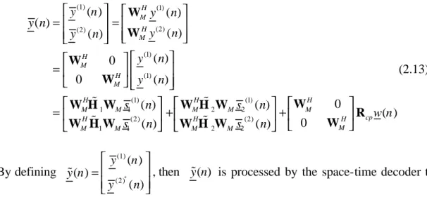
(1) (1) (2) (2) (1) (1) (1) (1) 1 1 2 2 (2) (2) 1 1 2 2 ( ) ( ) ( ) ( ) ( ) ( ) 0 0 ( ) 0 ( ) ( ) 0 ( ) ( ) H M H M H M H M H H H M M M M M H H H M M M M M y n y n y n y n y n y n y n s n s n s n s n     =  =    _ _       =_{ }     _{  }       =_{  }+ _{ }+ _       W W W W W W H W W H W W W H W W H W % % % % Rcpw n( ) (2.13) By defining _* (1) (2) ( ) ( ) ( ) y n y n y n     =    

% , then y n% is processed by the space-time decoder to ( ) produce the block z n( ) with diversity gains. Finally, the equalizer Γ is employed to recover s n( ). Then we can plot a frequency domain version of Fig. 2.1 in Fig.2.2.

ST Decoder Γ ( ) z n Decision ( ) y n% ( )n η ( ) s n _{s n}%_{( )} 1, 2 ? ? 1( ) s n 2( ) s n

Fig. 2.2 Frequency domain version of ST-OFDM transceiver

Here, we want to start with the following fact [18]:

Fact 1: The matrix H%_i can be diagonalized by pre- and post- multiplication with H M W and W , i.e., _M H ( ), M i M = Hi W H W% D (2.14)

where D(H_i) stands for the diagnal matrix with the vector H on its diagonal, and _i 0 ( ) ( ) L l i i l H ρ h l ρ− =

=

∑

is the frequency response of channel h(l) at point ρ which is different from the Toeplitz matrix H in Eq.(2.10). Moreover, we can write i

0 2 ( 1)/

[

(

j

),...,

(

j M M

)]

T

i i i i

H

=

V

h

=

H e

H e

π − (2.15)

with V denoting submatrix consisting of the first L+1 column of W_MH. ?

Exploiting Facts 1 and substitute Eq.(2.4), the vector y n in Eq.(2.13) can be ( ) written as: (1) (1) 1 1 2 2 (2) (2) 1 1 2 2 (1) (1) 1 1 2 2 (2) (2) 1 1 2 2 (1) 1 0 ( ) ( ) ( ) ( ) 0 ( ) ( ) ( ) ( ) ( ) ( ) ( ) ( ) ( ) ( ) ( ) ( ) H H H M M M M M cp H H H M M M M M s n s n y n w n s n s n H s n H s n v n H s n H s n H s       =_{  }+ _{ }+ _           =_{  }+ _+     = W W H W W H W R W W H W W H W D D D D D % % % % % * * (2) (1) 2 (2) (2) (1) 1 2 ( ) ( ) ( ) _{( )} ( ) ( ) ( ) ( ) ( ) n H s n _{v n} v n H s n H s n  +  _{ } +  _{  } − +       D D D % % % (2.16) where (1) (2) 0 ( ) ( ) ( ) 0 ( ) H M cp H M v n v n w n v n     =_{ =  }     W R W (2.17) Then,

* * * (1) (2) (1) (1) (2) 1 2 * (2) * (1) (2) 1 2 (1) (1) 1 2 * * (2) ₍₂₎ 2 1 ( ) ( ) ( ) ( ) ( ) ( ) ( ) ( ) ( ) ( ) ( ) ( ) _{( )} ( ) ( ) ( ) ( ) ( ) ( ) ( ) ( ) y n y n y n v n H s n H s n H s n H s n _{v n} v n H H s n H H s n v n     =        +  =_{ +  } − + _{ }  _{  }      =_{  }+ −     D D D D D D D D % % % % % % % = ( ) ( ) = ( ) ( ) = ( ) ( ) s n n s n n x n n η η η        Θ + + + D A (2.18)

where H, x n( ) and η( )n are defined, respectively, as

* (1) 2 * * ₍₂₎ 2 1 ( ) ( ) ( ) , ( ) ( ) ( ) _{( )} v n H H n H H η _{v n}     =_{  = }    _ _ 1 D D D D -D (2.19) , ( )x n s n( ), = Θ = A D A (2.20) When the channel matrices H and 1 H become available at the receiver, it is 2

possible to demodulate y n% with diversity gains by a simple matrix multiplication ( )

* 2 1 2 * * * 2 1 2 1 12 12 ( ) ( ) ( ) ( ) ( ) ( ) = ( ) ( ) ( ) ( ) ( ) ( ) = ( ) ( ) H H z n y n H H H H s n n H H H H s n n η ξ =     Θ +           ₊     1 1 2 D D D D D D D -D D -D D ? 0 0 D ? % (2.21) where * * 1 2 (H ) (H ) (H ) (H ) 12 1 2 D = D D + D D (2.22) ( )n H ( )n ξ =D η (2.23) We infer that multiantenna diversity of order two has been achieved because

2 2 2 2 12 1 1 | i(0)| , , | i( 1 ) | i i diag H H M = =   = _ − _ 

∑

∑

 D K (2.24)

inverse of _ _

 

12 1

12 2

D ? 0

0 D ? , which means the matrices D ? 12 i, i∈[1,2] need to be

full column rank. We can adopt the following design condition on the block lengths and the linear precoders to make sure the full rank of D ?12 i, [1,2]i∈ .

Condition 2.1) M > +K L.

Condition 2.2) ?i,i∈[1,2] is designed so that any K rows of ? are linearly i independent.

To select the appropriate precoders, we can construct them as Walsh code matrices. Then the soft decision data can be computed as:

12 1 12 2 ( ) ( ) ( ) s n = Γ ⋅z n =inv_ _z n     D ? 0 0 D ? (2.24) where 12 1 12 2 inv  Γ = _{ }     D ? 0 0 D ? (2.25)

Then we can project s n( ) onto the finite alphabet to obtain the hard decision discrete valuess nˆ( ).

However, we can adopt the precoder like [ ]

pre k

T T T

I I whereI_pre is formed by any

M-K rows of the K×K identity matrixI , as will be used in chapter 4. _k

In Eq.(2.20), we assume the channel information is already known at the receiver end, next we want to show how the channel become available in chapter 3.

Chapter 3

Blind Channel Estimation

In this chapter, we rely on M×K redundant linear precoders ? and ₁ ? ₂

(M >K to introduce redundancy) to show a blind channel estimation algorithm for Space-Time OFDM transmissions [17], and based on this channel estimation algorithm, we derive the theoretical mean square error of the estimator in section 3.2.

3.1 Subspace-based multichannel estimation

3.1.1 Noise free case

Before addressing the noisy case, we will start from the noiseless vectors x n( ) in Eq.(2.18):

( )=x n As n( ) (3.1) To estimate the channels, the receiver collects N blocks of x n( ) and forms a

2M ×N matrixX_N =[ (0),x K, (x N−1)], thus

XN =AS (3.2) N with S_N =[ (0),s K, (s N−1)]. At the receiver end, we also select the following [17]:

Condition 3.1) Note here the number of blocks N is large enough (≥2K) so that N

S has full rank 2K.

Condition 3.1) expresses the standard “persistence of excitation” assumption that is

satisfied by all signal constellations for N sufficiently large.

Condition 2.1) and Condition 2.2), together with Condition 3.1), and that s n( ) is a 2K×1 independent vector, imply that rank ( X )=2K, and the range space _N

( _N H_N) ( )

Range X X =Range A , and the nullity of X is _N 2M- 2K . Further, the singular value decomposition (SVD)

H x x N N x n H n   ∑  = = _{  }     V 0 X AS [U U ] V 0 0 (3.3)

with ∑x=diag(σ12,K,σ22k) and

2 2

1 2 k

σ ≥K≥σ , yielding the 2M×(2M −2 )K matrix U , whose columns span the null space _n N(X_N), which is caused by the redundant precoders.

Because N(X_N) is orthogonal to Range(X_N)= Range( )A , it follows that

2 1

0 for [1,2 2 ]

H T

k k

u A= _× k∈ M − K (3.4) where u_k is the null space vector stand ing for the kth column of U . _n

Let us now split the null space vector u_k into its upper and lower parts as ˆ_k

u

H k u A as _* 2_* 1 2 1 2 ( ) ( ) ˆ [ ] 0 ( ) ( ) H H T k k H H u u H H     =         1 D D ? 0 D -D 0 ? ( _(3.6)

Since for any M×1 vectors a and b it holds that

*

( ) ( )

H T

a D b = b D a , (3.7) Eq. (3.5) can be rewritten as

* 1 1 2 * * 2 ( ) ˆ ( ) ( ) [ ] 0 ˆ ( ) ( ) k T H k k T k k u u u H H u u =Ψ =  −   =         G ? 0 D D 0 ? D D ( ( 14243 144424443 (3.8) where 1 * 2   Ψ =     ? 0 0 ? , * * ˆ ( ) ( ) ( ) ˆ ( ) ( ) k k k k k u u u u u  −  =     D D G D D ( ( (3.9)

Plugging the Eq.(2.15) into Eq.(3.8), we have

* 1 2 * ( ) ˆ ( ) ( ) 0 [ ] 0 ˆ ( ) ( ) 0 k T T H k k T H k k u u u h h u u = ₌     − _{Ψ =}         F _G D D V D D V % ( ( 14243 144424443 (3.10) where 0 0 T H F=     V V (3.11)

In the above, we use Eq.(3.11) in time domain instead of Eq.(3.8) in frequency domain since it can make G u( _k)Ψ a smaller matrix which can reduce computatio n, and in Eq.(3.8) G u( k)Ψ cannot find the actual channel since it is not full rank.

Stacking Eq.(3.10) for each null space vector u_k with k∈[1,K, 2M−2 ]K , we obtain [ _{1 2} ] ( ₁) , , ( _{2 2} ) 0 H T H T J K h h h F_ u Ψ u ₋ Ψ =_ Q G G % K 1424_{3 1444442444443} (3.12)

where 1 2 2 ( ) , , ( _{J K}) F u u ₋  = _ Ψ Ψ_ Q G K G . (3.13) 1 2 [ ] H T H h% = h h (3.14) Hence, 2 ||h%HQ|| =h%HQQHh%=0 (3.15) Then, we can find the estimated channel h%ˆ as the eigenvector corresponding to the smallest eigenvalue of QQ : H

1

ˆ

argmin

eigenvector corresponding to the smallest eigenvalue of

H H h H h h h = = = QQ QQ % % % % (3.16)

The above algorithm is based on the null space U , so we name this algorithm _n

subspace-based channel estimation.

3.1.2 Noisy case

In the presence of white noise with variance 2 w

σ , we replace X in Eq.(3.3) by _N

N

Y , whose SVD has the following form:

H x x N x n H n n ∑    =     ∑     V 0 Y [U U ] V 0 % % % (3.17)

However, for large N,Y is replaced by the sample covariance matrix: N 2 2 1 1 ( ) ( ) H N H x x y x n H n n n y n y n N = ∑    = =     ∑    

∑

0 U R [U U ] U 0 % % % % (3.18)

following theorem [17]:

Theorem 1: Suppose Condition 2.1), Condition 2.2), and Condition 3.1) hold true;

let D denote any diagonal matrix with unit amplitude diagonal entries, and let

1, 2

Θ Θ be formed by any J−L rows of Θ Θ₁, ₂, respectively. If Θ₁ and Θ₂ satisfy

1 R( 2)

Θ ∉ Θ

D , the solution of [ 3 , 4 ] 0

T H T

h h Q= is unique up to a constant, and thus, channel identifiability within one scalar is guaranteed:

1 3 * 2 4 0 0 h h h h α α  ₌              I I (3.19)

Here we’ve assumed that (h h is a pair of channel satisfying Eq.(3.16). ? ₃, ₄)

We summarize the proposed subspace-based channel estimation algorithm [17] in the following steps.

Step 1) Collect the received data blocks y(n), and compute R_y% in Eq. (3.18). Step 2) Determine the eigenvectors u k_k, =1,K2M−2Kcorresponding to the

smallest eigenvalues of the matrix R_y%. Step 3) Build Q in Eq.(3.13).

Step 4) Determine the eigenvector corresponding to the smallest eigenvalue of QQ H

as our estimate in Eq.(3.16).

3.2 Performance Analysis of Mean Square Error

A performance analysis is conducted on the proposed estimator to derive the theoretical mean square error (MSE). Here we start from Theorem 2.

Theorem 2: Assuming that both noise and the signals are zero mean i.i.d. random

variables with variance σ_s2 and σ_w2, respectively, an approximation for the channel estimate’s MSE in Eq.(3.16) for high sample SNR and large sample size is

2 2 2 2 || || ˆ (|| || ) w s E h h N σ σ + − ≈ Q (3.20)

In the following, we want to prove Eq.(3.20) based on the first-order perturbation theory given in [19] in high SNR condition (small perturbation).

Lemma 1[19] : Assuming a matrix P permits the SVD

H p p p γ H γ   ∑  =       _{ }  V 0 P [U U ] V 0 0 (3.21)

and the perturbed matrix P% can be written as H p p p γ H γ γ ∑    = + ∆ = _{   } ∑    _{  }   V 0 P P P [U U ] V 0 % % % % % % (3.22) where n = n + ∆ n U% U U (3.23) γ is a vector of U_γ, then γHP=0, (3.24) the first-order approximation of the perturbation to the vector γ due to additive perturbation ∆P to γ is

γ − ∆+ Hγ

= P P

Deducing from lemma 1, since uk is the null space of XN, 0 H k N u X = , then H k N N k u =X+∆X u V (3.27) where 1 H N x x x + _{= ∑}− X U V (3.28) Moreover, from h%HQ =0 in Eq.(3.12.), the perturbation of the channel estimate is Vh= − ∆Q+ QHh (3.29) where the perturbation V to Q is additive and can be formed Q

1 2 2

( ) , , ( _{J K})

Q F u u ₋ 

∆ = _D V Ψ K D V Ψ_ (3.30) since F and Ψ are both deterministic.

In addition, the structure of V gives Q

(

)

1 2 1 2 2 1 2 1 2 2 * * 1 1 2 2 1 2 * 1 1 =[ ] ( ), , ( ) =[ ] ( ), , ( ) ˆ ˆ ( ) ( ) ( ) =[ ] , , ˆ ( ) ( ) H H H T H M K Q T H M K T H M K h h h h F u u H H u u u u u H H u u − =∆ − − =   Ψ     Ψ    −      Q Q G G G G D D D D D V V V K V 1444442444443 V K V ( K ( 2 2 * 2 2 2 2 2 2 1 * * 2 2 * * 2 1 2 1 1 2 2 ( ) ˆ ( ) ( ) ( ) ( ) ( ) ( ) = , , ( ) ( ) ( ) ( ) =[ , , ] M K M K M K H H M K H H M K u u u H H H H u u H H H H u u − − − − −   −   _{ Ψ}               _Ψ             Ψ 1 1 D D D D D D D D -D D -D D ( ( V K V % % V K V (3.31)

1 2 2 1 2 2 1 2 2 H H H H H M K H H H N N H H H N N M K H H H N N H H H H N N N M K u h u u u u u − + + − + + −  Ψ    =   Ψ     −Ψ ∆    =   _{−Ψ ∆}    Ψ   ∆      =      _Ψ  _{∆ ∆}      B d D Q D D X X D X X D X X D X X X V V V O M 1444442444443 144424443 (3.32) where 1 2 2 H H N H H N H N H H N N M K u u + + − Ψ    =    _Ψ     ∆    =   _{∆ ∆}    D X B D X X d X X O M (3.33)

Substituting Eq.(3.32) into Eq.(3.29) leads to

= H h + h + = −Q Q Q Bd V V (3.34)

Next, before computing the channel MSE, we prove the following lemma.

Lemma 2: Assume N is a matrix where each element is zero- mean i.i.d. random

variable with variance σ2

. Also assume J is an m m× deterministic matrix. Then

2

( H ) ( ) _n

E N JN =σ trace J I where I is an _n n n× identity matrix and trace( )⋅ gives

the trace of the matrix. ?

* 1 1 * 1 1 2 1 ( ) ( ) ( ) , 0, . m m ij ki kl lj l k m m kl ki lj l k m ll l E E E i j otherwise σ = = = = =    = _ ⋅ _⋅ _       = _ ⋅ ⋅ _    ₌  =  

∑ ∑

∑ ∑

∑

F N J N J N N J (3.35) Therefore, 2 2 1 ( ) ( ) . m H ll n n l E σ σ trace = =

∑

= N JN J I J I (3.36)

By using Lemma 2, it is easy to see that for the considered problem, we have

2 2 ( ) ( ) ( ) H H H N i j N i j n E u u trace u u i j σ σ δ ∆ ∆ = = − X X I I (3.37)

with δ( )⋅ being the Kronecker Delta function and, consequently

E(ddH)=σn2I (3.38) Then we can write estimated channel error covariance matrix

2 [ ] [ ] [ ] H H H H H H H H H n E h h E E σ + + + + + + ⋅ = = = Q Bdd B Q Q B dd B Q Q BB Q V V (3.39) where H H H H N N H H H N N + + + + _{Ψ Ψ}    =    _{Ψ Ψ}   D X X D BB D X X D O (3.40)

Here we assume that d is the only random variable.

In addition, to begin the derivation we recall that the unperturbed data X can be _N

written as X = D? S in Eq.(3.2) by setting N N Ψ = Θ ,which means we need to select ?₂ =?*₂. We define the data covariance matrix R as _x

H N N H H H N N x R = X X = D? S S ? D (3.41)

The generalized inverse of R is _x

1 ( ) ( ) ( ) H N N H H H N N + + + + − + X R = X X = ? D S S D? (3.42) Hence, we ha ve 1 1 ( ) ( ) ( ) H H H N N H H H H s H N N + + + − + − Ψ Ψ = Ψ Ψ = D X X D D ? D R D? D S S (3.43)

Therefore, Eq.(3.37) becomes

1 1 ( ) ( ) H N N H H N N − −     =       S S BB S S O (3.44)

For large N (number of data blocks), approximation

2 H

N N = Nσs

S S I (3.45) is reasonable, since we already assume that the signals are zero mean i.i.d. random variables. Thus 2 1 H s Nσ ≈ BB I (3.46)

Then Eq.(3.36) becomes

2 2 [ ] H H n s E h h N σ σ + + ⋅ ≈ ⋅ Q Q V V (3.47)

2 2 2 2 2 2 (|| || ) [ ( )] ( ) || || H H n s n s E h E trace h h trace N N σ σ σ σ + + + = ⋅ ⋅ ≈ ⋅ = Q Q Q V V V (3.48)

The closed form MSE expression Eq.(3.48) is compact and enables us to study the estimator’s performance dependence on the key system parameters— such as the input SNR, the number of data blocks. As expected, the MSE decreases with increasing input SNR and the number of received data blocks. This is later verified by comp uter simulation in Chapter 5.

CHAPTER 4

Improved Subspace Methods

To further improve the channel estimation, we can exploit the finite alphabet property to better the subspace-based channel estimates.

In this chapter, we discuss two different methods: decision direct (DD) [21] and phase direct (PD) [20]. DD, as implied in the name, needs first to get the hard decision data and then use it to update our estimated channel, while PD is to solve the phase ambiguities after we’ve got the channel power response. DD originally works in conventional OFDM, which only requires simple scalar division. Based on the space time data matrix, we extend it to ST-OFDM, which corresponds to a matrix inverse and multiplication because the received data is composed of two different transmitted data.

The main idea of PD is to solve the phase ambiguities after we get the channel power response. For conventional OFDM system, it is very easy to get the channel

them. So, the main problem we face now is how to get the channel power response. However, in general case the channel power response is hard to obtain. Hence, we only focus on BPSK system and exploit the transmitted data’s time and temporal correlation to develop a new algorithm named sum-difference square method to solve this problem.

Moreover, in time varying channel, we also need to choose a best window size to get the channel power response and apply it to PD. As we all know, when the window is longer, we can suppress the noise, but then we can’t follow the variance of the channel. This is the trade off. However, the choice of the window size is dependent on how fast the channel changes. Precoder design is another issue behind the algorithm as will be discussed in section 4.2.4.

4.1 Decision Direct (DD)

4.1.1 DD in ST-OFDM

In [21], Giannakis has shown how DD works in conventional OFDM, and we want to extend it to space time OFDM by using the space time data matrix.

There are four steps shown as follows:

Step (1) Set j=0, find an initial time domain channel estimate hˆ_{1,( )j} and hˆ_{2,( )j} using Eq.(3.16), calculate the frequency response Hˆ_{1,( )j} and Hˆ_{2,( )j} by Eq.(2.15). Step (2) Since now we have D1,( )j and D2,( )j , it is possible to detect s n( ) with

diversity gains by a simple matrix multiplication as Eq.(2.21) by substituting

1 2

(H ) and (H )

* 1,( ) 2,( ) * 2,( ) 1,( ) 12,( ) 12,( ) ( ) ( ) ( ) ( ) = ( ) ( ) ( ) ( ) = ( ) ( ) H j j H j j j j z n y n H H y n n H H s n n η ξ =   +         +     1 2 D D D D D -D D ? 0 0 D ? % % (4.1)

Then we can get the soft decision s n( ) as Eq.(2.24):

12,( ) 1 12,( ) 2 ( ) ( ) j ( ) j s n = Γ ⋅z n =inv_ _z n     D ? 0 0 D ? (4.2)

then we can project onto the finite alphabet to obtain the hard decision discrete values sˆ ( )_{( )j} n .

Eq.(4.2) shows how we collect soft decision data which corresponds to

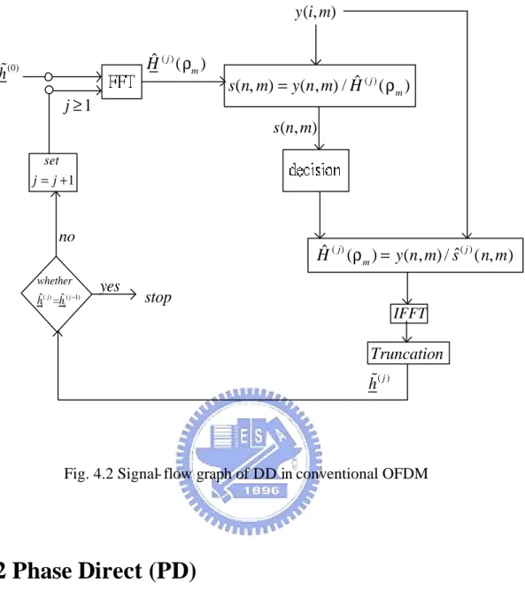
( ) ˆ( )

ˆ ( , )j ( , ) / j ( m)

s n m = y n m H ρ (4.3) in [20] for conventional OFDM which is only a simple one tap equalizer.

However in ST OFDM, we need first to get z n( ), the ST decoder output, and then feed it to equalizer Γ which compensates not only channel gain but also the precoder effect, hence it is more complicate.

Where y n m( , ) indicates the data for the mth subcarrier on the nth received data block, s n mˆ( , ) is the decision data corresponding to the mth subcarrier on the nth block, ˆH(ρ is the estimated frequency channel of the mth _m) subcarrier.

Step (3) Here, we separate step 3 to two parts. Part a) is to update the estimated channel from the decision data, and part b) is to update the detected data from the updated channel.

_{* *} (1) (2) (1) 1 2 (2) (2) (1) 1 2 ( ) ( ) ( ) ( ) ( ) ( ) ( ) s n s n v n y n v n s n s n  +    =_{− +  }+        D D D D % % % % (4.4)

Let D( )v stand for the diagonal matrix with the vector v, and define

(1) (1) (2) (2) ( ) ( ( )) ( ) ( ( )) n s n n s n = = S D S D % _% % _% (4.5) Since for J×1 vectors a and b it holds thatD( )a b=D( )b a, Eq.(4.3) can be rewritten as _{* *} (1) (2) (1) 1 2 (2) (2) (1) 1 2 ( ) ( ) _{( )} ( ) ( ) ( ) ( ) n H n H _{v n} y n v n n H n H  +  _{ } = _{ }+ _ − +       S S S S % % % % (4.6)

Apply the hard decision data to Eq.(4.6):

* * (1) (2) ₍₁₎ ( ) ( ) 1( ) (2) (2) (1) 2( ) ( ) ( ) ˆ _{( )} ˆ _{( ) ( )} ( ) ˆ _{( )} ˆ _{( ) ( )} j j j j j j n n H _{v n} y n H _{v n} n n  _{    }   = _{  }+ _ −        S S S S (4.7) where (1) ( ) 1 1,( ) ˆ _{( ) ( ˆ ( ))} j n = s j n S D ? and (2) ( ) 2 2,( ) ˆ _{( ) ( ˆ ( ))} j n = s j n S D ? (4.8)

Then we can simply get 1( )

2( ) j j H H       though Eq.(4.7) * * (1) (2) ( ) ( ) 1( ) (2) (1) 2( ) _{( ) ( )} ˆ _{( )} ˆ _{( )} ( ) ˆ _{( )} ˆ _{( )} j j j j _{j j} n n H inv y n H _{n n}     _{ } =   _{ − }     _{ } S S S S (4.9)

Update the time domain channel estimates

,( ) ,( )

H

i j i j

h =V H (4.10) and their frequency response using

,( ) ˆ,( )

ˆ

i j i j

H =Vh (4.11) Note that here Eq. (4.10) means to perform an M-point inverse DFT on

,( ) i j

we have assumed the channel delay spread is equal or less the n L); Eq. (4.11) amounts to performing an M-point DFT on an vector formed after zero-padding, we call Eqs.(4.10) and (4.11) denoising.

Eq.(4.9) is to update the estimated channel from the decision data which corresponds to

ˆH(ρm)= y n m( , ) / ( , )s n mˆ (4.12) in [20] for conventional OFDM.

(b) Check if hˆ_{i,( )j} ≅hˆ_i,(j−1), if yes, stop the iteration, if no , in each successive iteration, j is added by 1.

We have updated Hˆ_{i,( )j} in (a), then We can form D_{1,( )}j and D_{2,( )}j from 1,( )j = (Hˆ1,(j−1))

D D and D_{2,( )j} = (D Hˆ_1,(j−1)). Then, recompute the symbol estimates by Eqs.(4.1) and (4.2) to get the soft decision, and project again onto the finite alphabet to obtain hard decisionssˆ ( )_{( )j} n .

Step (4) Repeat Step (3).

(0) (0) 1 2 ˆ ˆ h and h FFT ( ) ( ) 1 2 ˆ j _and ˆ j H H ( ) y n% * 1,( ) , ( ) * 2 , ( ) ,( ) ( ) j j ( ) j j z n =  y n     2 1 D D D -D % 12,( ) 1 12,( ) 2 ( ) j ( ) j s n =inv__ __z n     D ? 0 0 D ? 12,( )j form D Decision * * (1) (2) ( ) ( ) (2) (1) ( ) ( ) ˆ _{( )} ˆ _{( )} ˆ _{( )} ˆ _{( )} j j j j n n form n n     −     S S S S * * (1) (2) ( ) ( ) 1( ) (2) (1) 2( ) _{( ) ( )} ˆ _{( )} ˆ _{( )} ( ) ˆ _{( )} ˆ _{( )} j j j j _{j j} n n H inv y n H _{n n}     _{ }   =   _{ } −     _{ } S S S S ( ) z n ( ) s n ( ) ˆ ( )_j s n ( ) y n * 1,( ) ,( ) * 2,( ) ,( ) j j j j form       2 1 D D D -D IFFT Truncation ( ) ( ) 1 2 ˆj ˆj h and h 0 j= 0 j> ( ) ( 1) ˆj₌ˆj i i whether h h − stop yes no 1 set j= +j

4.1.2 Comparison with conventional OFDM

We have shown how DD works in space time OFDM system, and the main equations are Eq.(4.2) and Eq.(4.9), while the former is to get the soft decision data, and the latter is to update the channel response while we have the decision data, both of which are corresponding to matrix inverse and multiplication. However, for DD in conventional OFDM [21], these two equations just become a simple scalar division, which are ˆ ˆ( , ) ( , ) / ( ) ˆ_{( ) ( , ) / ( , )ˆ} m m s n m y n m H H y n m s n m ρ ρ = = (4.13) where y n m( , ) indicates the data for mth subcarrier on the nth received data block,

ˆ( , )

s n m is the decision data corresponding to the mth subcarrier on the nth block, ˆ( _m)

H ρ is the estimated frequency channel of the mth subcarrier. See Fig.4.2 for

Signal- flow graph of DD in conventional OFDM. Eq.(4.13) is based on the well-known formula [1],

( , )y n m =H(ρ_m) ( , )s n m +n(ρ_m) (4.14) which leads to Eq.(4.13) a simple scalar division, but in space time OFDM, all the formulas are in matrix form which makes Eq.(4.2) and Eq.(4.9) both matrix inverse and multiplication. Note here that in Eq.(4.12) Γ corresponds to a psuedo inverse

since its size is 2M×2K, and in Eq.(4.9) * *

(1) (2) ( ) ( ) (2) (1) ( ) ( ) ˆ _{( )} ˆ _{( )} ˆ _{( )} ˆ _{( )} j j j j n n n n     −     S S S S

is full rank of size

( ) ˆ j _{( )} m H ρ (0) h% 1 j≥ ( ) ( 1) ˆj₌ˆj i i whether h h − stop yes no 1 set j= +j ( ) ˆ ( , ) ( , ) / j ( ) m s n m = y n m H ρ ( , ) y i m ( , ) s n m ( ) ˆ ( , )j s n m ( ) ( ) ˆ j _{( ) ( , ) / ˆ}j _{( , )} m H ρ = y n m s n m IFFT Truncation ( )j h%

Fig. 4.2 Signal- flow graph of DD in conventional OFDM

4.2 Phase Direct (PD)

4.2.1 Introduction of PD

Before addressing PD [20] to space time OFDM, we first show how it woks in conventional OFDM. Now, we start this part from Eq.(4.14), and focus on PSK constellation of size P:

{

2 /

}

1 P j p P P e _p π ζ = ₌ ,

We take the power of P to Eq. (4.14), omit noise for simplicity, and get the expectation

{ P( , )} {[ ( m) ( , )] }P P( m) { ( , )}P

In practice, E y i m{ ( , ) }P is replaced by sample averages and thus is estimated as 1 0 1 ( , ) ( ) { ( , )} N P P n m P y n m N H E s n m ρ − = =

∑

(4.16) where N is the received data block number.

Since we focus on PSK constellation of size P, we have E s{ O( , )} 1n m = . Hence, Eq.(4.16) becomes 1 0 1 ( ) ( , ) N P P m n H y n m N ρ − = =

∑

. (4.17) Hence, we’ve got the channel power response. Next, we only need to get the channel phase response, which means for each [0,m∈ M −1](assuming total M subcarriers ), we have 1/ ˆ( ) [ P( )] P m m m H ρ =λ H ρ (4.18) where λ_m∈

{

ej( 2 / )π P p, 1,...,p= P

}

(4.19) is the corresponding phase ambiguity in taking the Pth root.

For each m∈[0,M−1] , we can resolve the phase ambiguity by searching over candidate phase values

2 1/ argmin ( ) [ ( )] m P P m Hest m m H m λ λ = ρ −λ) ρ (4.20)

where H_est(ρ will be discussed in the following. _m)

Therefore, we can improve channel estimation accuracy through what we term Phase Directed (PD) steps that we describe next:

Step (2) In each successive iteration, j is added by 1, and

(a) Resolve phase ambiguities by replacing H_est(ρ with _m) H_(j−1)(ρ_m) in (4.20), and then form the vector

{

1/ 1/

}

0[ ( 0)] ,..., 1[ ( 1)]

P P P P

temp M M

H = λ H ρ λ ₋ H ρ ₋ (4.21)

(b) Update time domain channel estimates

( )

ˆ H

j temp

h =V H (4.22) and their frequency response using

( ) ˆ( )

ˆ

j j

H =V h (4.23) Step 3) Repeat Step2 several times, or continue until hˆ_{( )j} ≅hˆ_(j−1) within some tolerance.

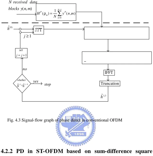
See Fig.4.3 for the signal- flow graph of phase direct in conventional OFDM.

The main difference between PD and DD is that DD alternates between channel estimation and symbol detection while PD avoids symbol estimation by decoupling channel estimation from symbol recovery. Therefore, PD is immune to the well-known error propagation phenomenon that is present in DD iterations.

( , ) N received data blocks y n m 1 0 1 ( ) ( , ) N P P m n H y n m N ρ − = =

∑

(0) h% Hest(ρm) _{1/ 2} argmin| ( ) [ ( )] | 0, , 1 m Q Q m est m m m get H H for m M λ λ = ρ −λ ρ = − ) K m λ

{

1/ 1/

}

0 0 [ P( )] P,..., [ P( )] P temp M M

phace compensated frequency response

H λ H ρ λ H ρ − = 0 j= IFFT Truncation 1 j≥ ( )j h% ( ) ( 1) ˆj₌ˆj i i whether h h − stop yes no 1 set j= +j

Fig. 4.3 Signal- flow graph of phase direct in conventional OFDM

4.2.2 PD in ST-OFDM based on sum-difference square

algorithm

Here, we want to apply PD to the Space- Time OFDM system. As described earlier, the main idea of PD is to solve the phase ambiguities in Eq.(4.20) after we get the channel power response Eq.(4.17). For conventional OFDM system, it is very easy to get the channel power response from (4.14). But here it is quite a different case, since the received data is composed of two different transmitted data as in Eq.(2.13); it’s not easy to separate them. So, he re we derive an algorithm to get the channel power

only use ±1 data in baseband since for other system it’s hard to solve the channel power response. Then we will get

(1) _{(1) (2) (1)} 1 2 (2) (1) (2) (2) 1 2 ( ) ( ) ( ) ( ) ( ) ( ) ( ) ( ) y n s n s n v n s n s n y n v n  _{  +   } = +  _{    } − +         D D D D % % % % (4.24)

For simplification, we only see the mth data part and omit noise.

(1) (1) (2) (2) (1) (1) (2) (2) 1 1 2 2 ( ) th data of ( ), ( ) th data of ( ) ( ) th data of ( ), ( ) th data of ( ) ( ) ( , ), ( ) ( , ) m m m m m m y n m y n y n m y n s n m s n s n m s n H ρ m m H ρ m m = = = = = D = D % % (4.25) Then we get (1) (1) (2) 1 2 (2) (2) (1) 1 2 ( ) ( ) ( ) ( ) ( ) ( ) ( ) ( ) ( ) ( ) m m m m m m m m m m y n H s n H s n y n H s n H s n ρ ρ ρ ρ = + = − + (4.26)

In the following, our purpose is to get H₁2(ρ_m) and H₂2(ρ_m) , the square of the channel frequency response. Square (4.26) and note that

(

s_m(1)( )n

) (

2 = s_m(2)( )n

)

2 =1 for BPSK

(

)

(

)

2 (1) 2 2 (1) (2) 1 2 1 2 2 (2) 2 2 (1) (2) 1 2 1 2 ( ) ( ) ( ) 2 ( ) ( ) ( ) ( ) ( ) ( ) ( ) 2 ( ) ( ) ( ) ( ) m m m m m m m m m m m m m m y n H H H H s n s n y n H H H H s n s n ρ ρ ρ ρ ρ ρ ρ ρ = + + = + − (4.27)

Here we adopt BPSK since we can have

(

sm(1)( )n

) (

2 = sm(2)( )n

)

2 =1. However if we adopt any PSK constellation of size P, we have to take the power of P to Eq. (4.26) to make

(

(1)

) (

( 2 )

)

( ) P ( ) P 1

m m

s n = s n = . Then it becomes very hard to solve, hence we only focus on BPSK.

By taking their sum and difference to Eq.(4.27), we have

(

) (

) (

)

(

) (

)

2 2 (1) (2) 2 2 1 2 2 2 (1) (2) (1) (2) 1 2 1 2 (4.28a) ( ) ( ) 2 ( ) ( ) ( ) ( ) 4 ( ) ( ) ( ) ( ) 4 ( ) ( ) m m m m m m m m m m m m y n y n H H y n y n H H s n s n H H ρ ρ ρ ρ ρ ρ + = + − = = ± (4.28b)