使用FPGA技術實現智慧型控制器於直流對直流電源轉換器

全文

(1)Implementation of Intelligent Control for DC-DC Power Converters Using FPGA Technology.

(2) 使用 FPGA 技術實現智慧型控制器於直流對直流電源轉換器. 研究生：王紹義. 指導教授：李祖添. 國立交通大學電機與控制工程系. 博士. 碩士班. 摘要本論文提出一個具有自我學習能力之模糊控制方法，整個控制法則包含一模糊規則調節器和一模糊控制器兩大部份，前者主要針對即時的輸出訊號誤差以及模糊推論運算決定規則調節量；後者主要將依據前者規則調節器產生的模糊規則來進行模糊運算求得所需之控制量。此方法的優點在於同時結合了即時線上學習的能力和模糊邏輯的特性，對於輸入變動或負載變動較大的受控系統有較佳的控制能力以及適應能力。最後，我們以 FPGA 實現此控制法則並運用在直流對直流電源轉換器上，經由實驗結果證明所提出之方法優於傳統 PI 控制器以及模糊控制器。. 關鍵字：自我學習模糊控制，模糊控制，FPGA 實現，直流對直流電源轉換器. I.

(3) Implementation of Intelligent Control for DC-DC Power Converters Using FPGA Technology. Student : Shao-Yi Wang. Advisor : Prof. Tsu-Tian Lee. Electrical and Control Engineering National Chiao Tung University. ABSTRACT In this thesis, a control strategy with the ability of self-learning, automatically-tuned fuzzy control is proposed. The proposed control strategy is composed of two parts—rule modifier and fuzzy controller. The rule modifier is designed to compute the modification of rules according to output error and fuzzy inference operation; the fuzzy controller is designed to decide the control effort of the modified fuzzy rules. The advantage of the proposed method is that it combines on-line real-time information and fuzzy control, so it achieves satisfactory control performance and has adaptability to large input variation and load variation of controlled plant. Finally, the control algorithm is implemented via FPGA. The experimental results show that the proposed control strategy can achieve better performance than PI control and fuzzy control do.. Key words: Self-learning fuzzy control, fuzzy control, FPGA implementation, DC-DC converters. II.

(4) 誌. 謝. 兩年的研究生涯很快就過去，首先要感謝李祖添老師給我機會，讓我有無限的資源以及學習的空間，使我在這兩年學到很多東西，再來要感謝我的父母的養育之恩，媽媽，您辛苦了；更要感謝許駿飛學長的指導及協助，讓我能快速的將論文完成。實驗室的同學徐彬桓，林宜甲在我需要幫忙時伸出援手，也使我的研究生活多采多姿。本篇論文不完美之處，還望各位先進多多指教。. III.

(5) Contents 摘要. I. ABSTRACT. II. 誌謝. III. Contents. IV. Contents of Figures. VI. Contents of Tables. VIII. Chapter 1 Introduction. 1. 1.1 General remark and overview of reviews. 1. 1.2 Contribution of the thesis. 3. 1.3 Scope of the Thesis. 4. Chapter 2 Modeling and Control of DC-DC Converters. 5. 2.1 Introduction of DC-DC converters. 5. 2.2 Modeling of forward DC-DC converter. 6. 2.3 Modeling of flyback DC-DC converter. 8. 2.4 Control of DC-DC converters. 10. Chapter 3 Intelligent Control Design for DC-DC Converters. 11. 3.1 Introduction of fuzzy control theory. 11. 3.2 Fuzzy controller design for DC-DC converters. 16. 3.3 Self-learning fuzzy controller design for DC-DC converters. 21. Chapter 4 FPGA-based Implementation. 25. 4.1 Introduction of DC-DC controlled system. 25. 4.2 Implementation of fuzzy control on FPGA. 27. IV.

(6) 4.3 Implementation of self-learning fuzzy control on FPGA. 37. Chapter 5 Experimental Results. 40. 5.1 Experimental descriptions. 40. 5.2 Experimental setup. 41. 5.3 Experimental results. 42. 5.4 Experimental discussions. 51. Chapter 6 Conclusion and Future Work. 52. 6.1 Conclusion. 52. 6.2 Future work. 52. References. 53. Appendix I. 57. Appendix II. 58. V.

(7) Contents of Figures. Fig. 1.1 Block diagram of the control system. 3. Fig. 2.1 Duty cycle of PWM. 6. Fig. 2.2 Forward DC-DC converter. 7. Fig. 2.3 Flyback DC-DC converter. 9. Fig. 3.1 Basic configuration of fuzzy control system. 11. Fig. 3.2 Min-product-max reasoning method. 15. Fig. 3.3 Simplified fuzzy reasoning method. 15. Fig. 3.4 Fuzzy controller of DC-DC converter. 17. Fig. 3.5 Membership functions of c and ce. 18. Fig. 3.6 Self-learning fuzzy control system. 21. Fig. 4.1 Overall FPGA control system. 25. Fig. 4.2 Membership functions of input variables e and ce (order). 28. Fig. 4.3 Membership functions of input variables e and ce (high/low). 28. Fig 4.4 Input variables e and ce storage data (low). 29. Fig. 4.5 Input variables e and ce storage data (high). 30. Fig. 4.6 Fuzzifier unit of input variables e and ce. 31. Fig. 4.7 Fuzzy rule values (gravity values). 32. Fig. 4.8 Fuzzy inference unit. 33. Fig. 4.9 Defuzzifier unit (COA method). 35. Fig. 4.10 Control unit simulation waveform (FC). 35. Fig. 4.11 Overall fuzzy control FPGA circuits. 36. Fig. 4.12 Control unit simulation waveform (SLFC). 38. Fig. 4.13 Overall self-learning fuzzy control FPGA circuits. 39. VI.

(8) Fig. 5.1 Experimental system picture. 41. Fig. 5.2 Experimental results of PI control for forward DC-DC converter. 43. Fig. 5.3 Experimental results of fuzzy control for forward DC-DC converter. 44. Fig. 5.4 Experimental results of self-learning fuzzy control for forward DC-DC converter. 45-46. Fig. 5.5 Experimental results of PI control for flyback DC-DC converter. 47. Fig. 5.6 Experimental results of fuzzy control for flyback DC-DC converter. 48. Fig. 5.7 Experimental results of self-learning fuzzy control for flyback DC-DC converter. 49-50. VII.

(9) Contents of Tables. Table 3.1 Fuzzy rules of the DC-DC converters. 21. Table 4.1 Specification of DC-DC Converters. 25. Table 4.2: Input variable e and ce storage data (order). 28. Table 4.3 ROM of fuzzy rule values. 32. Table 4.4 Multiplexer of four effective fuzzy rules. 33. Table 4.5 Learned fuzzy rules at the first time. 37. Table 4.6 Comparison of hardware resource requirement for. 40. PI control, FC and SLFC Table 6.1 The comparison of the experimental results. VIII. 51.

(10) Chapter 1 Introduction. 1.1 General remark and overview of reviews The DC-DC converters are power electronic systems that convert one level of electrical voltage into another level by switching action [1-3]. The DC-DC converters have been used widely in our common lives and in industrial manufactory, such as, desktop PCs, notebooks, office automations, industrial computers, networking devices etc. The control technique for the DC-DC converter must cope with their wide input voltage and load variations to ensure stability in any operating condition while providing fast transient response. For many years, the control approaches are limited to PI controller structures based on the traditional frequency domain methods [4-6]. Recently, a series of papers have considered the control of the DC-DC converters based on robust control theory [7, 8], sliding-mode control approach [9-11] and fuzzy control(FC) technique [12-17]. In the feedback linearization control design, its performance generally depends on the working point. In the sliding-mode control design, the system model is required for the controller design. In the fuzzy control design, too many fuzzy rules need to be constructed by trial-and-error tuning procedure. Fuzzy control using linguistic information possesses several advantages such as robustness, model-free, universal approximation theorem and rule-based algorithm. However, most of the design of fuzzy rules has relied on the knowledge of the expert and via the trial-and-error design process. Recently, the developed design using adaptive techniques [18-20] and genetic algorithms [21, 22] have provided another approach for FC design. In [18-20], a FC design method based on the Lyapunov synthesis approach has been studied. The key element is the merger of adaptive. 1.

(11) systems with fuzzy approximation theory, where the fuzzy system can approximate the unknown control system dynamics or controllers. With these approaches, the fuzzy rules can be automatically adjusted to achieve satisfactory system response by some dynamic adaptation laws. However, these design methods always need a complex analysis and heavy computation load. In [21, 22], a FC design method that used the genetic algorithm to find the membership functions and the rule sets was proposed. The genetic algorithm design method can be used to learn different types of fuzzy rules, including fuzzy rules with singleton consequent, fuzzy rules with fuzzy set consequent, and linear-equations fuzzy rules. However, this design method lacks the on-line adaptation ability to meet the variations of the controlled plant or changing environments. From these present studies about control algorithms for DC-DC converters, fuzzy control has shown that the method is proper because of its fast and precise computing. Fuzzy control is based on expert knowledge and human language to form control algorithms and does not need any complicated mathematical models. The self-learning approach is presented in this paper in order to obtain more adaptability of different power converter plant models. The ways to implement a fuzzy system using microcontroller technique for DC-DC converters have been used for a long time [10, 25, 26]. But the microcontroller lacks flexibility of hardware implementation. In the recent studies, implementation of control algorithms on field programmable gate array (FPGA) becomes more and more popular [28-30]. And it shows the feasibility and flexibility of the control algorithms. We use FPGA to implement our controller because it is (1) easily implemented and verified, (2) high sampling rate and switching frequency, (3) without using a PWM IC (the PWM signal is easily generated by FPGA), (4) able to control the DC-DC converter in different FPGA boards with the same VHDL code.. 2.

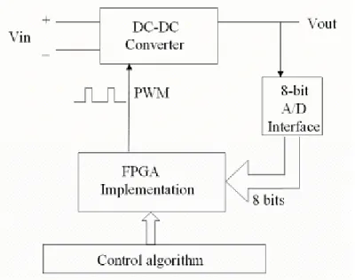
(12) 1.2 Contribution of the thesis The motivation of this thesis is to design a self-learning fuzzy control (SLFC) system for the DC-DC converters on an FPGA development board. The proposed SLFC system using a back-propagation method is expressed. The proposed SLFC system contains two sets of fuzzy inference logic; one is the fuzzy controller and the other is the rule modifier. The rule modifier is a fuzzy learning algorithm that will modify the control rules. The modification value of each rule is based on the fuzzy firing weight, so that the fuzzy learning algorithm can proceed reasonably and quickly. Then, the proposed SLFC system can automatically tune the fuzzy rules to achieve satisfactory performance. We will show the response of PI control, fuzzy control, and self-learning control. And the results show that the SLFC is indeed better than the others. The idea of this study is to design an intelligent control PWM chip based on the FPGA. And we make it possible to implement the fuzzy and self-learning fuzzy control on an FPGA. The input of the FPGA is an 8-bit A/D Vout data and the output of the FPGA is a one-bit PWM signal. The block diagram of the developed FPGA-based experimental setup is shown in Fig. 1.1.. Fig. 1.1 Block diagram of the control system. 3.

(13) 1.3 Scope of the Thesis In this thesis, we will show the mathematical models of two common DC-DC converters: forward and flyback type converters in Chapter 2. Forward converters drop the input voltage and flyback ones pull up and drop input voltage. In Chapter 3, we will introduce the fuzzy control algorithm and the self-learning fuzzy control algorithm. Then we will show the hardware implementation via FPGA of the fuzzy control and self-learning fuzzy control in Chapter 4.. The. experimental results, including the PI controller, the fuzzy controller and the self-learning fuzzy controller, are compared in Chapter 5. Finally, conclusion and future work are given in Chapter 6.. 4.

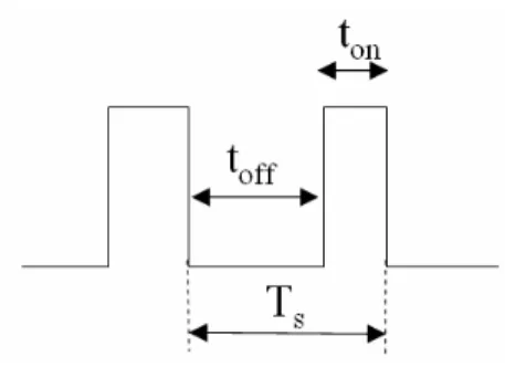
(14) Chapter 2 Modeling and Control of DC-DC Converters. 2.1 Introduction of DC-DC converters DC-DC converters have two categories: (1) basic-type converters (2) derivative-type converters. Basic-type converters have no electrical isolation between input and output, and there is only one active power transistor in the DC-DC converter circuit. Generally, the bipolar junction transistor (BJT), metal-oxide semiconductor field-effect transistor (MOSFET) and insulated gate bipolar transistor (IGBT) are the most common power transistors. Basic-type converters include the buck-type (step down) converter and the boost-type (step up) converter. Derivative-type converters have electrical isolation between input and output, and there are one or more active power transistors in the DC-DC converter circuit. Derivative-type converters include flyback, forward, push-up, half -bridge and full-bridge converters. Switching power converters could control the average output voltage by setting the on-time ton and off-time toff of the power transistor within the specific input voltage range. In other words, the average value of output voltage is decided by ton and toff with certain switching period ( Ts= ton + toff ). We could control its average output voltage by adjusting on-time ton of the power transistor. The control strategy is called the Pulse-Width Modulation, PWM. And we call the ratio of ton and Ts the duty cycle. Duty cycle (D) = ton/Ts. Fig. 2.1 depicts the duty cycle.. 5.

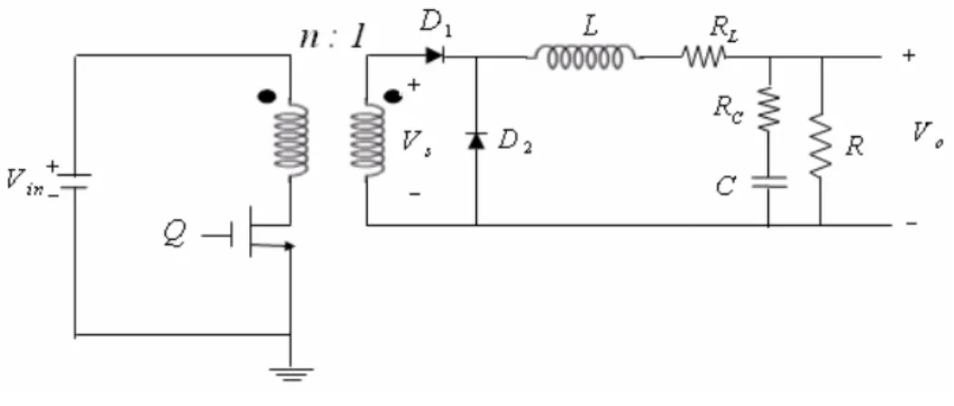
(15) Fig. 2.1 Duty cycle of PWM The forward DC-DC converter and flyback DC-DC converter are introduced in the next two paragraphs. The output voltage of the forward DC-DC converter is smaller than input voltage, and the output voltage of flyback DC-DC converter can be either higher or lower than input voltage. These are the plants we will propose to examine the control algorithm in this thesis.. 2.2 Modeling of forward DC-DC converter A forward DC-DC converter, which can provide isolation between input and output and is commonly used at power levels up to about 5kW, is shown in simplified form, open-loop, in Fig. 2.2. The transformer provides both isolation and the possibility of a very wide output voltage range. During the transistor on-time, diode D1 is forward biased, and energy is transferred from the input voltage to the output load resistance R. During the off-time, diode D1 is reversed biased and diode D2 is forward biased to maintain continuous current of the output voltage. An inductance L in the circuit is an energy-storage element during the switching action. The low-pass filter across the output voltage included an capacitance C and a resistor Rc in order to keep the output voltage close to constant between the transistor on-time and off-time. The two situations of the power transistor are discussed separately.. 6.

(16) Fig. 2.2 Forward DC-DC converter (1). When the transistor Q is on, the transformer is induced a voltage Vs. Diode D1 is on and diode D2 is off. We can neglect the voltage drop across diode D1 if Vo is much larger than 5V. If the change of current of inductance L is ∆iL , the voltage across L is (neglect the voltage drop of RC and RL) Vs − Vo = L. ∆iL ton. (2.1). And ∆iL can be rewritten as ∆iL =. Vs − Vo ton L. (2.2). (2). When the transistor Q is off, D1 is off and D2 is on. And the D2 forward biased voltage is also neglected. The output voltage is. Vo = L. ∆iL toff. (2.3). And the change of current ∆iL of L is ∆iL =. Vo toff L. (2.4). The change of current of inductance L is the same whether ON or OFF of the transistor. So. 7.

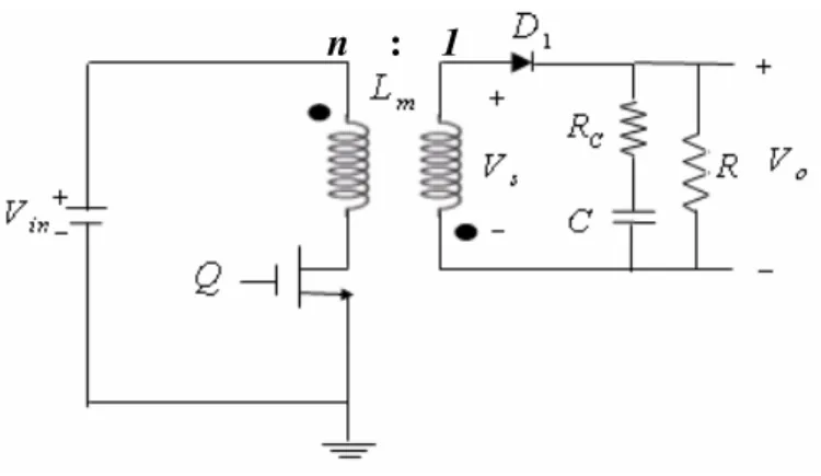
(17) Vs − Vo V ton = o toff L L. (2.5). Substituting Vs = Vin / n, ton = D Ts , and toff = (1-D) Ts, we obtain Vo D = Vin n. (2.6). where n is the ratio of the transformer induction coil, D is the duty cycle of PWM signal. The forward type DC-DC converter is used to drop the dc voltages. The circuit of a forward type DC-DC converter is shown in the previous page, where C is output capacitance, L is inductance, R is load resistance, RL is inductance series resistance, RC is capacitance series resistance, Vin is input voltage, and Vo is output voltage. From [23], we can obtain the transfer function in continuous conduction mode as Vo ( s ) 1 + SRC C = nD Vin ( s ) S 2 LC + S ( RC + RL ) C + L. R. +1. (2.7). From this transfer function, we can apply the frequency domain analysis to determine the parameters of the PI controller.. 2.3 Modeling of flyback DC-DC converter The flyback DC-DC converter is a buck-boost type converter with electrical isolation [3]. The flyback converter can be developed as an extension of the buck-boost converter. Fig. 2.3 shows the basic converter topology. It replaces the inductance of buck-boost converter by a transformer. The buck-boost converter works by storing energy in the inductance during the ON phase and releasing it to the output during the OFF phase. With the transformer the energy storage is in the magnetization of the transformer core.. 8.

(18) n. : 1. Fig. 2.3 Flyback DC-DC converter The magnetic element is not really a transformer; it is used to transfer energy as a coupling inductance. The most important point of the circuit is to store and release the magnetic energy. The advantage of this type DC-DC converter is that it is low cost, simple structure, and easy to obtain multiple output voltage. Therefore, it is often used to aid the design of power supply. We omitted the circuit derivation of the flyback converter [3], the relation between input and output of an ideal forward DC-DC converter is. Vo 1 D = ⋅ Vin n 1 − D. (2.8). Also from reference [23], the transfer function of the flyback DC-DC converter between input and output voltage in continuous conduction mode is. Vo ( s ) = Vin ( s ). n n2 +S S Lm C (1 − D)2 2. D (1 + SRC C ) (1 − D) Lm n 2 n2 +1 RC + RL C+ R (1 − D) 2 (1 − D) 2. (2.9). where Lm is the magnetizing inductance of the transformer. We can apply the final value theorem to examine the steady-state value as (2.8) shows. In the same way, the frequency domain analysis method is also applied to the flyback converter in order to obtain the suitable parameters of PI controller.. 9.

(19) 2.4 Control of DC-DC converters The popular technique of the DC-DC converters is pulse-width modulation (PWM), where the switching frequency is constant and the duty cycle, D (k ) , varies with the load resistance variations at the k-th sampling time. The output of the designed controller, δ D (k ) , is the change of the duty cycle. Then, the duty cycle is determined by adding the previous duty cycle D (k − 1) to the calculated change in duty cycle. D (k ) = D (k − 1) + δ D (k ) .. (2.10). The calculated duty cycle signal is then sent to a PWM output stage that generates the appropriate switching pattern for the power switch(transistor) in the DC-DC converter. The control problem of the DC-DC converter is to control the duty cycle so that the output voltage Vo (k ) can provide a fixed voltage under the occurrence of the uncertainties such as the wide input voltage and load variations. The output error voltage is defined as. e(k ) = Vref − Vo (k ) .. (2.11). where V ref is the output voltage command. The control law of the duty cycle is determined by the error voltage signal to provide fast transient response and small overshoot in the output voltage. The control algorithms will be introduced in Chapter 3.. 10.

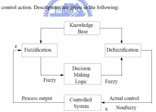
(20) Chapter 3 Intelligent Control Design for DC-DC Converters. 3.1 Introduction of fuzzy control theory The general structure of fuzzy controller (FC), represented in Fig. 3.1, comprises four principle components: (1). A fuzzification which converts input data into suitable linguistic values; (2). A knowledge-base which consists of a data base with the necessary linguistic definitions and control rule set; (3). A decision-making logic which simulates a human decision process, infers the fuzzy control action from the knowledge of the control rules and the linguistic variable definitions; and (4). A defuzzification which yields a nonfuzzy control action from an inferred fuzzy control action. Descriptions are given in the following:. Fig. 3.1 Basic configuration of fuzzy control system 3.1.1 Fuzzification Fuzzification could be defined as a mapping from an observed input space to fuzzy sets in certain input universe of discourse. Fuzzification plays an important role in dealing with 11.

(21) uncertain information. In fuzzy control applications, the observed data are usually crisp. Since the data manipulation in a FC system is based in fuzzy set theory, fuzzification is necessary during an earlier stage. However, the fuzzification interface always involves the following functions: (1) Determine the values of input variables. (2) Performs a scale mapping that transfers the range of values of input variables into corresponding universe of discourse. (3) Converts input data into suitable linguistic values, which may be viewed as labels of fuzzy sets. Suppose that the part of the control rules takes inputs from the sensor readings, which are usually real numbers. These real-valued sensor measurements are matched to their corresponding fuzzy variables by finding the matching membership values.. 3.1.2 Knowledge base In general, the design of FC is based on the operators understanding of the behavior of the process instead of its detailed mathematical model. The main advantage of this approach is that it is easy to implement a significant experience and heuristics. On the other hand, based on this view it is difficult to automate the design process. Nevertheless, there are a few guidelines for selecting control rules. Rules can be derived in several ways, including the following: a. Based on the expert experience or knowledge base. The database provides necessary definitions, which are used to define linguistic control rules and fuzzy data manipulation in a FC system. These concepts are based on experience and engineering judgment. b. Based on observing the operator’s control action. It should be noted that the correct choice of the membership functions of a term set plays an 12.

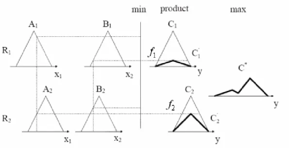
(22) essential role in the success of an application. c. Based on learning algorithms. The rules base characterizes the control goals and control policy of the domain experts by means of a set of linguistic control rules. In other words, a fuzzy system is characterized by a set of linguistic statements based on expert knowledge. The expert knowledge is usually in the form of “if - then” rules, which are easily implemented by fuzzy conditional statements in fuzzy logic. The collection of fuzzy control rules that are expressed as fuzzy conditional statements forms the rule base of the rule set of a FC system.. 3.1.3 Decision making logic The decision-making logic is the kernel of FC, it has the capability of simulating human decision-making base on fuzzy concepts and of inferring fuzzy control actions employing fuzzy implication and the rules of inference in fuzzy logic. In general, fuzzy reasoning is based on a compositional rule of inference, which can be viewed as an approximate extension of the modus ponens. Herein two most popular fuzzy reasoning methods are discussed. (1) Min-product-max method For simplicity, assume that we have two fuzzy control rules as follow Rule 1: If x1 is A1 and x2 is B1 then y is C1. (3.1). Rule 2: If x1 is A2 and x2 is B2 then y is C2 Given x1 is x1’ and x2 is x2’, where x1’ and x2’ are real numbers. Then the firing weights f1 and f2 can be represented as. f1 = u A1 ( x1 ' ) ∗ u B1 ( x2 ' ). (3.2). f 2 = u A2 ( x1 ' ) ∗ u B2 ( x2 ' ). (3.3). 13.

(23) where * represents the product inference.. ( y ) and The output of each control rule from its action part is represented by the fuzzy sets C1 ' C2 ' ( y ) and is given by C1 ' ( y ) = f1 ∧ C1 ( y ). (3.4). C2 ' ( y ) = f 2 ∧ C2 ( y ). (3.5). where ∧ is the minimum operation. Then the output membership function uc(y) is written as. uc ( y ) = C1 ' ( y ) ∪ C2 ' ( y). (3.6). where ∪ represents the maximum operation. Fig.3.2 shows the min-product-max reasoning method. (2) Simplified reasoning method As a special case of the Min-product-max method, we can give a simplified fuzzy reasoning method. For the following fuzzy reasoning form: Rule 1:. A1 and B1. C1. Rule 2:. A2 and B2. C2. Rule n:. An and Bn. Cn. (3.7). In which the consequent parts of the fuzzy rules are not fuzzy sets but real number C1, C2, … , Cn in y , called the fuzzy singleton . Fig.3.3 shows the consequence y0 by the simplified fuzzy reasoning method. The degree of the fact [x1 and x2] to the antecedent part (Ai and Bi) is given as. f i = u Ai ( x1 ) ∗ u Bi ( x2 ). (3.8). The firing weight fi, may be regarded as the degree with which Ci is obtained.. 14.

(24) Fig. 3.2 Min-product-max reasoning method. Fig. 3.3 Simplified fuzzy reasoning method 3.1.4 Defuzzification The defuzzification inference performs the following functions: (1) A scale mapping, which converts the range of output variables into corresponding universe discourse. (2) Defuzzification, which yields a nonfuzzy control action from an inferred fuzzy control action. The purpose of the defuzzification process is to transform the output of the inference, which. 15.

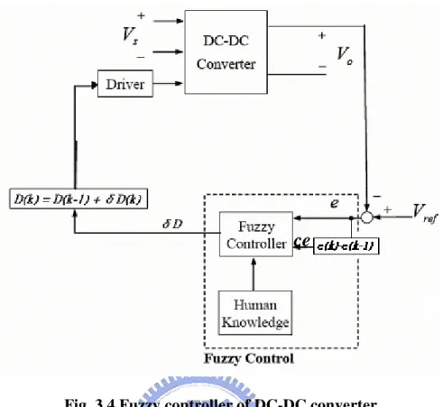
(25) is a fuzzy set to a crisp value so that it could be used to control a process. There are many ways to defuzzify the inference results but we use the most common method, called the Center-of-Area (COA) method and (3.9) is the COA method. n. y0 =. 1. fi ∗ C i n. (3.9). fi. 1. where y0 is the crisp output value, control action. A simplified fuzzy reasoning method, which operation schemes are shown in Fig. 3.3. The final consequence of simplified fuzzy reasoning method is obtained as the weighted average of C1, C2 by the firing weight f1, f2.(COA method). y0 =. f1 ∗ C1 + f 2 ∗ C2 C1 + C2. (3.10). In the general form, the defuzzification result is. y0 =. f 1 ∗ C 1 + f 2 ∗ C 2 + ... + f n ∗ C n f 1 + f 2 + ... + f n. (3.11). 3.2 Fuzzy controller design for DC-DC converters The block diagram of the fuzzy control scheme of DC-DC converters is shown in Fig. 3.4. The fuzzy controller is divided into two parts: fuzzy controller and human knowledge. The inputs of the fuzzy controller are the error (e) and the change of error (ce), which are defined as (2.13) and. ce = e(k ) − e(k − 1). (3.12). (3.12) denotes the change of error is that the difference between the present error and the last sampling-time error.. 16.

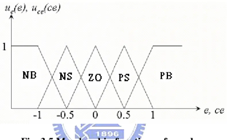
(26) ce. Fig. 3.4 Fuzzy controller of DC-DC converter In order to reduce the computation, the fuzzy variables e and ce are described by fuzzy singletons, meaning that the measured values of these variables are used in the inference process without being fuzzified. Specifically the fuzzy rules are in the form. Ri : IF e(k ) is Ai and ce(k ) is Bi , then δ D (k ) is Ci. (3.13). where Ai and Bi are fuzzy subsets in their universes of discourse, and Ci is a fuzzy singleton. Each universe of discourse is divided into five fuzzy subsets: (1). PB: Positive Big, (2). PS: Positive Small, (3). ZO: Zero, (4). NS: Negative Small, (5). NB: Negative Big. 17.

(27) The partition of fuzzy subsets and the shape of the membership function are shown in Fig. 3.5. The values of e and ce are normalized. The triangular shape of the membership function of this arrangement presumes that there is only one dominant fuzzy subset for any particular input. Also for any combination of e and ce, a maximum of four rules are adopted. The computation time can thus be further reduced. For example, if e is 0.1 and ce is -0.7, only (ZO, NS), (ZO, NB), (PS, NS), and (PS, NB) are in effect. The inferred grades of membership of the rest of the rules are zero.. Fig. 3.5 Membership functions of c and ce The derivation of the fuzzy control rules is heuristic in nature and based on the following criteria: (1) When the output of the converter is far from the set point, the change of duty cycle must be large so as to bring the output to the set point quickly. (2) When the output of the converter is approaching the set point, a small change of duty cycle is necessary. (3) When the output of the converter is near the set point and is approaching it rapidly, the duty cycle must be kept constant so as to prevent overshoot. (4) When the set point is reached and the output is still changing, the duty cycle must be changed a little bit to prevent the output from moving away.. 18.

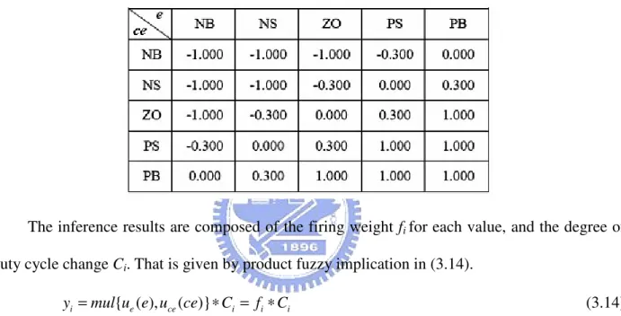
(28) (5) When the set point is reached and the output is steady, the duty cycle remains unchanged. (6) When the output is above the set point, the sign of the change of duty cycle must be negative, and vice versa. According to these criteria, a rule table is derived and shown in Table 3.1, where the fuzzy rules are normalized between -1 and 1.. Table 3.1 Fuzzy rules of the DC-DC converters. The inference results are composed of the firing weight fi for each value, and the degree of duty cycle change Ci. That is given by product fuzzy implication in (3.14).. yi = mul{ue (e), uce (ce)} ∗ Ci = fi ∗ Ci. (3.14). where mul{*} represents multiplication or product operation. yi is the change of duty cycle inference by the ith rule. As yi of (3.14) is the linguistic result, it is necessary to transfer the result into the output of the fuzzy controller through the defuzzification procedure. The defuzzification result can be written as (3.15) by using the COA method. 4. δ D(k ) =. i =1 4 i =1. yi fi. 4. =. i =1. f i ∗ Ci 4 i =1. (3.15). fi. The output of the fuzzy controller is the duty cycle and is defined as. D (k ) = D (k − 1) + λ ⋅ δ D (k ). (3.16) 19.

(29) where δ D (k ) is the inferred change of duty cycle by the fuzzy controller at the kth sampling time, and λ is the gain factor of the fuzzy controller. Adjusting λ can change the effective gain of the controller. Then the inferred value D(k) of the control action is applied to control the converter. In summary, the principle of fuzzy control algorithm is described as follows: 1. Sample the output signal of the plant. 2. Calculate the error and change of error. 3. Determine the fuzzy subset and membership function for error and change of error. 4. Determine the change of control action according to the individual fuzzy rule. 5. Calculate the actual change of control action by defuzzification operation. 6. Send the change of control action (PWM) to control the converter.. 20.

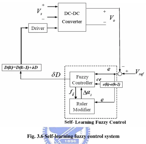
(30) 3.3 Self-learning fuzzy controller design for DC-DC converters. Fig. 3.6 Self-learning fuzzy control system In the above section, the fuzzy rules shown in Table 3.1 should be determined by time-consuming trial-and-error tuning procedure, and no one knows if they are the best control rules to achieve favorable control performance. In this section, the self-learning fuzzy control(SLFC) design method will be proposed such that the fuzzy rules can be automatically learned and the system can achieve favorable control performance. The block diagram of self-learning fuzzy control for a DC-DC converter is shown in Fig. 3.6. It is composed of two parts:(1)fuzzy controller and (2) rule modifier. Considering the fuzzy control rules given in (3.13), an iterative learning algorithm is adopted to adjust the control actions. The central part of the iterative learning algorithm for a SLFC system is to change the control action in the direction of the negative first-order derivative (to rule values) of a cost function E which is defined as following 21.

(31) E (k ) =. 1 ⋅ e( k ) 2 2. (3.17). where e(k) is the error function. By using the concept of back-propagation neural network method, we minimize the energy function. When E is approaching to zero, the error is also approaching to zero. The system achieves the target. Then the rule is generated as. α i (k + 1) = α i (k ) − η ⋅ where. ∂E (k ) ∂α i (k ). (3.18). 1 is the learning rate. And substitute E (k ) = e(k ) 2 and e(k ) = Vref − Vo , we get 2 1 ∂ e( k ) 2 −∂Vo (k ) ∂E (k ) = 2 = e( k ) ⋅ ∂α i (k ) ∂α i (k ) ∂α i (k ) −∂Vo (k ) ∂[δ D (k )] = e( k ) ⋅ ⋅ (3.19) ∂[δ D (k )] ∂α i (k ). ∂Vo can be calculated by the type of converter. As the ∂[δ D (k )] fi ⋅ αi i and substitute controlled converter is a forward type converter. Substitute δ D (k ) = fi. From (3.19), the Jacobin term. D (k + 1) = D(k ) + δ D(k ) , the (3.19) can be rewritten as fi ⋅ α i i ∂ 1 fi ∂ ⋅ Vin ⋅ D(k + 1) ∂E (k ) n i = −e ( k ) ⋅ ⋅ ∂[δ D(k )] ∂α i (k ) ∂α i (k ). i. ∂[ D(k ) + δ D(k )] f i 1 = −e(k ) ⋅ Vin ⋅ ⋅ n fi ∂[δ D(k )] i. f 1 = −e(k ) ⋅ ⋅ Vin ⋅ i n fi. (3.20). i. So the self-learning fuzzy controller rule modifier of forward type converter is. fi. 1 n. α i (k + 1) = α i (k ) − (−η ⋅ e(k ) ⋅ ⋅Vin ⋅. fi i. 22. ). (3.21).

(32) Moreover, as the controlled converter is a flyback type converter, the (3.19) can be rewritten as. fi ⋅ α i. D(k + 1) ∂ 1 ∂ ⋅ Vin ⋅ fi ∂E (k ) 1 − D(k + 1) n i = − e( k ) ⋅ ⋅ ∂[δ D (k )] ∂α i (k ) ∂α i (k ) i. 1 = −e(k ) ⋅ Vin ⋅ n. ∂. D(k ) + δ D(k ) 1 − D(k ) − δ D(k ) f ⋅ i fi ∂[δ D(k )] i. f 1 1 = −e(k ) ⋅ ⋅ Vin ⋅ ⋅ i 2 n fi [1 − D(k ) − δ D(k )]. (3.22). i. Therefore, SLFC rule modifier of flyback type converter is. 1 n. α i (k + 1) = α i (k ) − (−η ⋅ e(k ) ⋅ ⋅Vin ⋅. f 1 ⋅ i ) 2 fi [1 − D(k ) − δ D(k )]. (3.23). i. The actual meaning of (3.21) and (3.23) is when error function is minimized, we have to minus the first-order derivative to rule values of E(k). (The error is as small as possible when the desire output voltage is reached.) The rule modifier. i. is negative learning rate when Vo > Vref ,. and positive learning rate when Vo < Vref. We could rewrite (3.21) and (3.23) into (3.24), where. 1 n. 1 n. η ' represents the term η ⋅ ⋅Vin in (3.21) and the term η ⋅ ⋅Vin ⋅ when considering them as constants. The term. 1 in (3.23), [1 − D(k ) − δ D(k )]2. 1 is approximated as constant [1 − D(k ) − δ D(k )]2. when δ D(k ) is very small.. fi. α i (k + 1) = α i (k ) − (−η ' ⋅ e( k ) ⋅. fi. ). (3.24). i. α i (k + 1) = α i (k ) − δα i (k ). (3.25). 23.

(33) where δα i is a modification value to be added to the i-th control rule in (3.13). Equation (3.24) shows that the modification value of each control rule is proportional to real-time error and firing weight of fuzzy inference. And the defuzzification of the controller output is given as 4. δD =. i =1. fi ∗ α i 4. i =1. (3.26). fi. where f i is the firing weight of the i-th rule. In summary, the fuzzy rules of SLFC are given in (3.13) with the control actions α i updated with (3.24). In the design of the FC system, the fuzzy rules should be pre-constructed to achieve the design performance by trial and error; however, this trial-and-error tuning procedure is time consuming. The proposed SLFC system can automatically tune the fuzzy rules to achieve satisfactory performance. In summary, the principle of self-learning fuzzy control algorithm is described as follows: 1. Sample the output signal of the plant. 2. Calculate the error and change of error. 3. Determine the fuzzy subset and membership function for error and change of error. 4. Calculate the self-learning fuzzy rules according to real-time error and inference results. 5. Determine the change of control action according to the new-learned fuzzy rules. 6. Calculate the actual change of control action by defuzzification operation. 7. Send the change of control action (PWM) to control the converter.. 24.

(34) Chapter 4 FPGA-based Implementation. 4.1 Introduction of DC-DC controlled system In the Fig. 4.1, the feedback voltage is transformed into an 8-bit digital signal by ADC0804. The 8-bit signal is transferred to FPGA board. And after one-sampling-period computation of control algorithm, a 1-bit PWM output is connected to the gate of the power MOS of the DC-DC converter to control the reference voltage. We implement the control algorithms on FPGA using VHDL(very high speed ICs hardware description language) [31, 32] Table 4.1 is the converter specification, including the forward and flyback type converters, and the picture of the two type converters are shown in Appendix I.. Fig. 4.1 Overall FPGA control system. 25.

(35) Table 4.1 Specifications of DC-DC Converters. Some hardware that are required for implementation are presented as following.. FPGA (ALTERA stratix series: EP1S10F780C6) The FPGA board we use is the NIOS II development board of ALTERA company. It can be also taken as an embedded system board. We will show the board picture and some specifications in Appendix II. The reason why we use FPGA to implement the control algorithm for DC-DC converters is that (1) FPGA can generate PWM without a PWM IC, (2) Switching DC-DC converters need high switching frequency, (3) The DC-DC converters require high precision so the control action must be very fast. (4) The digital control sampling rate can be very fast to handle the variation of the power converter system. Among all the reasons, we choose FPGA to implement our controller.. ADC0804 The feedback voltage signal is the analog signal, so we have to transform it into the digital signal for digital control system. ADC0804 is a 8-bits A/D converter IC and is the most commonly used.. 74LS07 It is a digital signal buffer IC. It is necessary to prevent the reverse current of the power transistor from destroying the FPGA board. 26.

(36) 4.2 Implementation of fuzzy control on FPGA The fuzzy controller circuit contains four parts – “fuzzifier unit”, “inference unit”, “defuzzifier unit” and “control unit”. The specifications are as following: (1) The fuzzy chip has 2 inputs (e and ce) and 1 output (PWM). (2) The precision of the membership functions is 8 bits (0~255). (3) The precision of the membership degree is 6 bits (0~63). (4) Each input variable (e or ce) corresponds to 5 membership functions. (5) The overlapped number of every membership function is 2. (6) There are 25 fuzzy rules. (7) We use COA(center of area) method in the defuzzifier unit. (8) Membership functions and gravity values(fuzzy rules) are saved in ROMs.. 4.2.1 Design of fuzzifier unit The main job of fuzzifier is to transform crisp value of e and ce into corresponding information of membership functions. Then decide the inference value and gravity value to compute the two values in the defuzzifier unit. We use two ROMs to save the information about how to transform the crisp values into fuzzy data. Input values are taken as memory addresses.. 4.2.1.1 The way to save input membership functions Due to the symmetric triangular membership functions in the fuzzifier unit, the way we save addresses and data is the same. In order to control the target voltage without much oscillation, we have to set the membership function near zero (ZO) thinner and make the membership functions away from zero fatter. Fig. 4.2 and 4.3 show the membership function data of input variables (e and ce), which the number of membership functions is 5 and overlapped 27.

(37) number is 2. Then we classify four orders:”000” “001” “010” “100”, and every order includes “low” and “high” two parts, where “low” or “high” means the decrease or increase side of every membership function. Data “order”, “low”, and “high” are saved in the form of 3-bit memory. The total memory space we need in the fuzzifier unit is two 255*9-bit ROMs—ROM1 and ROM2. The actual memory mapping of “order” is listed in Table 4.2. Fig. 4.4 and Fig. 4.5 represent the memory mapping of “low” and “high” respectively, but we only show the coarse line for simplicity. Others not mentioned in these figures can be obtained via the same way.. Fig. 4.2 Membership functions of input variables e and ce (order). low. high. Fig. 4.3 Membership functions of input variables e and ce (high/low). Table 4.2: Input variable e and ce storage data (order). 28.

(38) Fig 4.4 Input variables e and ce storage data (low). 29.

(39) Fig. 4.5 Input variables e and ce storage data (high). 30.

(40) 4.2.1.2 Working principle of fuzzifier unit Fig. 4.6 shows the block diagrams of fuzzifier unit— e and ce (up and down). It clearly shows that the block diagram is composed of multiplexer, ROM and control signals.. Fig. 4.6 Fuzzifier unit of input variables e and ce The control unit gwnerates a signal to multiplexer to take e and ce as address bus, and it also generates a trigged signal to read data from ROM at the same time. The data read from ROM are “order”, “high”, and “low”, where “order” becomes “order_1” through the increment circuit. Signals “order” and “order_1” represent membership functions of input variables (such as NB, PS etc.) and “low” represents the membership degree of “order”, “high” represents the membership degree of “order_1”. Then transfer these data to inference unit.. 31.

(41) 4.2.2 Design of inference unit 4.2.2.1 The way to save data of fuzzy output. Fig. 4.7 Fuzzy rule values (gravity values). Fig. 4.7 shows the fuzzy rule values (Ci). The fuzzy rule values are also called gravity values (gi) in this thesis. The normalized control actions from -1 to +1 are mapping to 8-bit data 0~255, so the fuzzy singleton values in Table 3.1 are -1, -0.3, 0, +0.3, +1 corresponding to 0, 89, 127, 165, and 255. These values are saved in a ROM. Table 4.3 shows the memory mapping of fuzzy rule table in Table 3.1. Every gravity value is an 8-bit data saved in a 6-bit address. So we need 25x6 bits for memory storage of the fuzzy rule table.. Table 4.3 ROM of fuzzy rule values. 32.

(42) 4.2.2.2. Working principle of inference unit. Fig. 4.8 shows the inference unit. Inference unit receives 3-bit data — included “order”, “order_1”, “low” and “high” from fuzzifier unit. Because the fuzzy controller has 2 inputs and 2 overlaps, there are 4 rules in effect during every sampling time. There are two values gi and fi generated in the inference unit: (1). gi: Combine signals “order1”, “order1_1”, “order2” and “order2_1”, such as “001”&“100”. “001100”. After a multiplexer process we obtain 4. addresses corresponding to 4 gravity values, gi, saved in a ROM. (2). fi: Multiply signals “low” and “high” in turn via a multiplexer in the Product block to generate firing weights, fi. Then send the values “gi” and “fi” to defuzzifier unit. The multiplexer selects different data by a 2-bit control signal— “s”, which is shown in Table 4.4.. Fig. 4.8 Fuzzy inference unit. Table 4.4 Multiplexer of four effective fuzzy rules. 33.

(43) 4.2.3 Design of defuzzifier unit The COA method is applied to the defuzzifier unit. It deals with the firing weight fi and gravity value gi from inference unit and generates a crisp output control action. The crisp control action is as following 4. y0 =. fi ∗gi. i =1. 4. (4.1). fi. i =1. where y0 is the crisp control action of the PWM signal. Fig. 4.9 is the block diagram of the defuzzifier unit (COA method), gi is the fuzzy rule values, fi is the firing weight. At first, the two values multiply with each other. Then, send the value to the accumulator after a multiplier. The accumulator is composed of an adder and a register. When the trigger signal ‘load’ is at the rising edge, add the value saved in the register. fi equals to unity (63 in binary) so we don’t need a divider in this design. Just shift 6 bits and get an 8-bit result (for example: 01101100100101 four times, shift the result of meaning is to divide. fi*gi right. 01101100). After accumulating. fi*gi right 6 bits using combinational logic, where the actual. fi*gi by 64(unity). After the defuzzifier unit, we multiply a scale factor to. the 8-bit control action signals. In the end, we send the control action values to change the duty cycle of a PWM signal. Thus, one-sampling-time computation is done.. 34.

(44) Fig. 4.9 Defuzzifier unit (COA method) 4.2.4. Design of control unit Control unit produces the sequential synchronized signals. The signals are shown at Fig.. 4.10. They are simulated with Quartus. simulator. Signal ‘clk’ is an input clock with 50 MHz. freguency. And rst, sample, sample1, I_clk, load, load1, div, and s are the signals generated by ‘clk’.. Fig. 4.10 Control unit simulation waveform (FC). 4.2.5 Fuzzy controller overall circuit diagram Fuzzy control FPGA circuits are shown in Fig. 4.11. They are all implemented in VHDL. ROM1 and ROM2 blocks are the process of fuzzification—it is the memory of addresses and. 35.

(45) data of input membership functions. Blocks MUX, Product and ROM3 are the process of the inference engine—it computes the product inference and read the gravity values in turn with four different “s”. The last blocks MUL, OUTSF, and DUTY are the defuzzification process doing the jobs of multiplying and accumulating, multiplying a suitable output scale factor, and generating the PWM signal respectively. The control block is responsible for the trigger signals in order to synchronize the process. The number of logic elements (LEs) for fuzzy control system design is 950.. Fig. 4.11 Overall fuzzy control FPGA circuits. 36.

(46) 4.3 Implementation of self-learning fuzzy control on FPGA From (3.24) and (3.25), it can be observed that the self-learning fuzzy control algorithm is:. fi. α i (k + 1) = α i (k ) − (−η ' ⋅ e( k ) ⋅. fi. ). (3.24). i. In short, the current rule value α i is modified by a minus term of δα i . The equation is rewritten as:. α i (k + 1) = α i (k ) − δα i (k ). (3.25). The fuzzy rule values(gravity values) are set as zeros initially. Then the controller generates 4 gravity values in effect every sampling time by (3.24) or (3.25). The defuzzifier process is the same as the fuzzy controller. As shown in Table 4.5, for instance, four rules (8, 10, 18, and 20) are in effect in the first sampling time. The zero values of these effective rules are replaced by 18,. and. 20. 8,. 10,. respectively after the algorithm is applied. Then the four learned rule values are sent. to the ROM of defuzzifier unit and decide the control actions to the DC-DC converter.. Table 4.5 Learned fuzzy rules at the first time. The implementation of SLFC on FPGA is different from FC in several ways: (1) ROM3 block updates every sampling time.. fi. ⋅ e( k ) ⋅ (2) The signal “learn0” represents the term – η '. fi i. 37. in (3.24)..

(47) fi. Where signal “err0” is e(k ) , “y2” is. fi. , and after multiplying each other along with. i. learning rate η ' in MUL block, it generates signal “learn0”. (3) The fuzzy rule values (gravity values)—gi is generated by “learn0” and “err0”. The meaning of “learn0” is the modification value of rule modifier ( −δα i (k ) ). We choose “learn0” as 0~7(000~111) to modify the fuzzy rule values in this thesis. When “err0”>127, add “learn0” to the corresponding gravity values; while “err0”<127 subtract “learn0” from the corresponding gravity values. (4) The fuzzy rule table is modified recursively by (3.24), and the modified fuzzy rule values are sent to inference and defuzzifier unit to decide the control action. The number of logic elements(LEs) of the SLFC system design is 2,478. The control unit simulation waveform is shown in Fig. 4.12 via Quartus II, and the overall SLFC circuits are shown in Fig. 4.13.. Fig. 4.12 Control unit simulation waveform (SLFC). 38.

(48) Fig. 4.13 Overall self-learning fuzzy control FPGA circuits. 39.

(49) At last, we make a comparison table of hardware implementation on FPGA of three control methods. Table 4.6 shows the comparison of the hardware resource requirement of each method. Total number of logic elements (LEs) is 10,570. Total number of pins is 427. Total number of memory bits is 920,448.. Table 4.6 Comparison of hardware resource requirement for PI control, FC and SLFC. 40.

(50) Chapter 5 Experimental Results. 5.2 Experimental setup The proposed control algorithms are realized on an FPGA using VHDL. The DC-DC converter plants are forward and flyback DC-DC converters. The VHDL code is compiled on the software platform of Quartus II 4.0 into a *.cdf file and the file is downloaded to the FPGA board through USB JTAG. The FPGA board is NIOS II embedded system development board of ALTERA company. The processor type number is EP1S10F780C6. In short, the overall system is inclusive of an FPGA board, controlled DC-DC converter, A/D interface, power supply, and a programming and download computer. The picture of the system is shown in Fig. 5.1.. forward / flyback DC-DC converters A/D interface. FPGA board. Fig. 5.1 Experimental system setup. 41.

(51) 5.2 Experimental descriptions There are three control algorithms we implement on FPGA, inclusive of PI control, fuzzy control(FC), self-learning fuzzy control(SLFC). In order to test the adaptability of different input voltages, we choose 50V and 60V as input voltages. Two tests in this experiment are described as following. (1). Transient-response test is to set output voltage from 10V to 15V after some duration. (2). Load-variation test is to set load resistance from 0. to 100. in a period of time.. Fig. 5.2~5.4 are forward converter responses, while Fig. 5.5~5.7 are flyback ones. On the top of each figure is the output response of controlled plant and on the bottom of that is the control action. Next, we describe the forward-converter experiments. The responses of PI controller are shown in Fig. 5.2(a)~(d), reference output voltage(Vref) of Fig. 5.2(a) is 10V in the beginning and 15V after some duration. Fig. 5.2(b) is the experimental result of load-variation test. The timing of the load-changing point (from 0. to 100. ) is pointed out in every. load-variation test. Fig5.2(c), (d) with 60V input voltage corresponds to Fig. 5.2(a), (b). Fuzzy control responses are shown in Fig.5.3(a)~(d). Self-learning fuzzy control responses are depicted in Fig. 5.4(a)~(h), where the fuzzy rules of (a) are set as zeros initially, while those of (b) are learned. The reference output voltages(Vo) of Fig. 5.4(a), (b) are 15V and 20V, and Fig. 5.4(c), (d) are load-variation tests with initially not learned and learned fuzzy rules. Fig. 5.4(e)~(h) with 60V input voltage corresponds to Fig. 5.4(a)~(d). Flyback converter experimental results are in the same order of forward ones. p.s. The control action is an 8-bit output from OUTSF block and we measure it via a DAC0804, which is a digital to analog converter IC.. 42.

(52) 5.3 Experimental results The unit of output response is 10V/div, and control action is 5V/div. The time interval is 400ms/div. And the timing of load-variation test is pointed out in the following figures.. load variation. output response. output response. 15V. 10V. 10V. control action. control action 5V. 400ms. (a). (b). Input: 50V ; Output: 10V & 15V. load-variation test Input: 50V; Output: 10V. load variation output response. output response. control action. control action. (c). (d). Input: 60V ; Output: 10V & 15V. load-variation test Input: 60V; Output: 10V. Fig. 5.2 Experimental results of PI control for forward DC-DC converter KP=0.13, KI=0.016. 43.

(53) load variation output response. 15V. 10V. 5V. output response. 10V. control action. control action. 400ms. (a). (b). Input: 50V ; Output: 10V & 15V. load-variation test Input: 50V; Output: 10V. load variation. output response. output response. control action. control action. (c). (d). Input: 60V ; Output: 10V & 15V. load-variation test Input: 60V; Output: 10V. Fig. 5.3 Experimental results of fuzzy control for forward DC-DC converter. 44.

(54) output response. output response. 20V. 15V. 15V. control action. 5V. control action. 400ms. (a). (b). Input: 50V ; Output: 15V & 20V. Input: 50V ; Output: 15V & 20V. Fuzzy rules have not been learned. Fuzzy rules have been learned. load variation. load variation. output response. output response. 15V. control action. control action. (c). (d). load-variation test. load-variation test. Input: 50V ; Output: 15V. Input: 50V ; Output: 15V. Fuzzy rules have not been learned. Fuzzy rules have been learned. Fig. 5.4 Experimental results of self-learning fuzzy control for forward DC-DC converter. η '=0.03125. 45.

(55) output response. 20V. 15V. 5V. output response. control action. control action. 400ms. (e). (f). Input: 60V ; Output: 15V & 20V. Input: 60V ; Output: 15V & 20V. Fuzzy rules have not been learned. Fuzzy rules have been learned. load variation. load variation. output response. output response. 15V. control action. control action. (g). (h). load-variation test. load-variation test. Input: 60V ; Output: 15V. Input: 60V ; Output: 15V. Fuzzy rules have not been learned. Fuzzy rules have been learned. Fig. 5.4 Experimental results of self-learning fuzzy control for forward DC-DC converter (Cont.). η '=0.03125. 46.

(56) load variation output response. output response. 15V. 10V. 10V. 400ms 5V. control action. control action. (a). (b). Input: 50V ; Output: 10V & 15V. load-variation test Input: 50V; Output: 10V. load variation output response. output response. control action. control action. (c). (d). Input: 60V ; Output: 10V & 15V. load-variation test Input: 60V; Output: 10V. Fig. 5.5 Experimental results of PI control for flyback DC-DC converter KP=0.5, KI=0.063. 47.

(57) load variation output response. output response. 15V. 10V. 10V. 400ms 5V. control action. control action. (a). (b). Input: 50V ; Output: 10V & 15V. load-variation test Input: 50V; Output: 10V. load variation output response. output response. control action. control action. (c). (d). Input: 60V ; Output: 10V & 15V. load-variation test Input: 60V; Output: 10V. Fig. 5.6 Experimental results of fuzzy control for flyback DC-DC converter. 48.

(58) output response. output response. 15V. 10V 400ms 5V. control action. control action. (a). (b). Input: 50V ; Output: 10V & 15V. Input: 50V ; Output: 10V & 15V. Fuzzy rules have not been learned. Fuzzy rules have been learned. load variation. load variation. output response. output response. 10V. control action. control action. (c). (d). load-variation test. load-variation test. Input: 50V ; Output: 10V. Input: 50V ; Output: 10V. Fuzzy rules have not been learned. Fuzzy rules have been learned. Fig. 5.7 Experimental results of self-learning fuzzy control for flyback DC-DC converter. η '=0.03125. 49.

(59) output response. output response. 15V. 10V 400ms 5V. control action. control action. (e). (f). Input: 60V ; Output: 10V & 15V. Input: 60V ; Output: 10V & 15V. Fuzzy rules have not been learned. Fuzzy rules have been learned. load variation. load variation. output response. output response. 10V. control action. control action. (g). (h). load-variation test. load-variation test. Input: 60V ; Output: 10V. Input: 60V ; Output: 10V. Fuzzy rules have not been learned. Fuzzy rules have been learned. Fig. 5.7 Experimental results of self-learning fuzzy control for flyback DC-DC converter (Cont.). η '=0.03125. 50.

(60) 6.4 Experimental discussions (1). Experimental results show that fuzzy control achieve better transient response than PI control. And self-learning fuzzy control has more adaptability of load-variation test. In other words, the steady state of SLFC is more stable and smooth than others. (2). Self-learning fuzzy control has smaller overshoot after learning algorithm is applied. (3). Transient oscillation is obvious in the first time when the SLFC is applied, after the rules are modified by the learning algorithm, the oscillatory condition has been improved. (4). The flyback type DC-DC converter plant achieves better performance than the forward one, because input and output scale factors of the fuzzy controller are more suitable for the flyback converter system. (5). The reason why the forward converter does not achieve ideal performance is that the scale factors of the fuzzy controller have not been suitably chosen. Table 6.1 shows the comparison of experimental results for three methods.. Table 6.1 The comparison of the experimental results. 51.

(61) Chapter 6 Conclusion and Future Work 6.1 Conclusion This thesis has demonstrated the self-learning fuzzy control(SLFC) system for forward type and flyback type DC-DC conveters, where the new type control algorithm SLFC has been developed in which the rule bases do not need to be prior defined. The SLFC design method can automatically generate the rule bases to achieve better performance. In the rule modifier, the modification value is obtained from fuzzy inference of modification rules so that the learning algorithm can proceed reasonably and quickly. Experimental results have been provided to demonstrate the robust control performance of the proposed control systems under the occurrence of uncertainties.. 6.2 Future Work In the future, we can apply other intelligent control strategy to implement the DC-DC converters on the FPGA board. Such as, sliding-mode self-learning control and other adaptive fuzzy control, etc. In this thesis, the FPGA implementation of the proposed control method is more complicated than PI control and fuzzy control. So what we have to do is to reduce the chip area of the FPGA processor. So the SLFC control algorithm needs to be simplified in order to make the SLFC more efficient and low cost.. 52.

(62) References [1] R. D. Middlebrook and S. Cuk, Advances in Switched-Mode Power Conversion, Pasadena, Teslaco, 1981. [2] N. Mohan, Tore M. Undeland and William P. Robbins, Power electronics : converters, applications, and design, John Wiley & Sons, 1989. [3] H. W. Whittington, B. W. Flynn and D. E. Macpherson, Switched mode power supplies : Design and construction, Wiley, 1992. [4] A. Luchetta, S. Manetti, M.C. Piccirilli and A. Reatti, “Frequency domain analysis of DC-DC converters using a symbolic approach,” IEEE Trans. Circuits and Syst., vol. 3, pp. 2043-2046, May 1995. [5] N. Femia and M. Vitelli, “Frequency domain analysis of DC-DC converters with internally controlled switching instants,” IEEE Power Electron. Congress, pp. 269–276, Oct. 1996. [6] J. Alvarez-Ramirez, I. Cervantes, G. Espinosa-Perez, P. Maya and A. Morales, “A stable design of PI control for DC-DC converters with an RHS zero,” IEEE Trans. Circuits and Syst. I, vol. 48, pp. 103 - 106, Jan. 2001. [7] J A. Kugi and K. Schlacher, “Nonlinear H ∞ -controller design for a DC-to-DC power converter,” IEEE Trans. Control Syst. Technol., vol. 7, pp. 230-237, Mar. 1999. [8] E. Vidal-Idiarte, L. Martínez-Salamero, H. Valderrama-Blavi, F. Guinjoan and J. Maixé, “Analysis and design of H ∞ control of nonminimum phase-switching converters,” IEEE Trans. Circuits and Syst. I, vol. 50, pp. 1316-1323, Oct. 2003. [9] S. K. Mazumder, A. H. Nayfeh and D. Borojevic, “Robust control of parallel DC–DC buck converters by combining integral-variable-structure and multiple-sliding-surface control schemes,” IEEE Trans. Power Electron., vol. 17, pp. 428-437, May 2002.. 53.

(63) [10] S. L. Jung, M. Y. Chang, J. Y. Jyang, H. S. Huang, L. C. Yeh and Y. Y. Tzou, “Design and implementation of an FPGA-based control IC for the single-phase PWM inverter used in an UPS”, Power Electron. and Drive Syst. Conference vol.1, pp. 344–349, May 1997. [11] M. Lopez, L. G. Vicuna, M. Castilla, P. Gaya and O. Lopez, “Current distribution control design for paralleled DC/DC converters using sliding-mode control,” IEEE Trans. Ind. Electron., vol. 51, pp. 419-428, April 2004. [12] C. C. Lee, “Fuzzy logic in control systems: fuzzy logic controller-part I/II,” IEEE Trans. Syst., Man and Cybern., vol. 20, pp. 404-435, March 1990. [13] Lin, B.-R., “Analysis of fuzzy control method applied to DC-DC converter control”, APEC '93. Conference Proceedings, pp. 22–28, March 1993. [14] J. R. Timothy, Fuzzy Logic with Engineering Application, McGraw-Hill, New York, 1995. [15] W. C. So, C. K. Tse and Y. S. Lee, “Development of a fuzzy logic controller for dc/dc converters: design, computer simulation and experimental evaluation,” IEEE Trans. Power Electron., vol. 11, pp. 24-32, Jan. 1996. [16] L. X. Wang, A Course in Fuzzy Systems and Control, Prentice-Hall, Englewood Cliffs, New Jersey, 1997. [17] A. Balestrino, A. Landi and L. Sani, “Cuk converter global control via fuzzy logic and scaling factors,” IEEE Trans. Ind. Appl., vol. 38, pp. 406-413, March 2002. [18] L. X. Wang, Adaptive Fuzzy Systems and Control - Design and Stability Analysis, Prentice-Hall, Englewood Cliffs, New Jersey, 1994. [19] H. Lee and M. Tomizuka, “Robust adaptive control using a universal approximator for SISO nonlinear systems,” IEEE Trans. Fuzzy Syst., vol. 8, pp. 95-106, Jan. 2000. [20] S. D. Wang and C. K. Lin, “Adaptive tuning of the fuzzy controller for robots,” Fuzzy Sets and Syst., vol. 110, pp. 351-363, March 2000. 54.

(64) [21] A. Homaifar and E. McCormick, “Simultaneous design of membership functions and rule sets for fuzzy controllers using genetic algorithms,” IEEE Trans. Fuzzy Syst., vol. 3, pp. 129-139, May 1995. [22] C. F. Juang, J. Y. Lin and C. T. Lin, “Genetic reinforcement learning through symbiotic evolution for fuzzy controller design,” IEEE Trans. Syst., Man and Cybern., Pt B, vol. 30, pp. 290-301, April 2000. [23] A. Barrado, E. Olias and A. Lazaro, “PWM-PD Multiple Output DC/DC Converters : operation and control-loop modeling,” IEEE Trans., Power Electron., vol. 19, pp. 140-149 , January 2004. [24] P. T. Krein, J. Bentsman, R. M. Bass and B. L. Lesieutre, “On the use of averaging for the analysis of power electronic systems,” IEEE Trans. Power Electron., vol. 5, pp. 182-190, April 1990. [25] T. Gupta, R. R. Boudreaux, R. M. Nelms and J. Y. Hung, “Implementation of a fuzzy controller for dc-dc converters using an inexpensive 8-b microcontroller”, IEEE Trans. Ind. Electron., vol. 44, pp. 661-669, Oct. 1997. [26] R. R. Boudreaux, R. M. Nelms, and J. Y. Hung, “Simulation and modeling of a DC-DC converter controlled by an 8-bit microcontroller,” APEC '97 Conference Proceedings, vol.2 pp. 963–969, Feb 1997. [27] E. Vidal-Ldiarte, L. Martine-Salamero, F. Guinjoan, J. Calvente and S. Gomariz, “Sliding and fuzzy control of a boot converter using an 8-bit microcontroller,” IEEE Proc., Electron. Power Appl., vol. 151, pp. 5-11, Jun. 2004. [28] S. L. Jung, M. Y. Chang, J. Y. Jyang, L. C. Yeh and Y. Y. Tzou, “Design and implementation of an FPGA-based control IC for AC-voltage regulation”, Power Electron. and Drive Syst. Conference, vol.14, pp. 522–532, May 1999. 55.

(65) [29] F. M. Yasin, A. Tio, M. S. Islam; M. I. Reaz and M. S. Sulaiman, “The hardware design of temperature controller based on fuzzy logic for industrial application employing FPGA”, Microelectron. 16th Conf., pp. 157-160, Dec. 2004. [30] The website of AlTERA company: http://www.altera.com. [31]. , VHDL. [32]. ,. ,. , 1999.. VHDL. ,. 56. , 1999.

(66) Appendix I Two kinds of DC-DC converters in the thesis (1). Forward DC-DC converter:. (2). Flyback DC-DC converter:. 57.

(67) Appendix II AlTERA NIOS II development board:. Features and specifications: A StratixTM EP1S10F780C6 device 8 Mbytes of flash memory 1 Mbyte of static RAM 16 Mbytes of SDRAM On board logic for configuring the Stratix device from flash memory On-board Ethernet MAC/PHY device Two 5-V-tolerant expansion/prototype headers each with access to 41 Stratix user I/O pins Compact FlashTM connector header for Type I Compact Flash (CF) cards Mictor connector for hardware and software debug Two RS-232 DB9 serial ports Four push-button switches connected to Stratix user I/O pins Eight LEDs connected to Stratix user I/O pins Dual 7-segment LED display JTAG connectors to Altera® devices via Altera download cables 50 MHz oscillator and zero-skew clock distribution circuitry Power-on reset circuitry. 58.

(68) Nios Development Board, Stratix Edition Block Diagram:. 59.

(69)