Simplifying the valuation of reverse annuity mortgages
不動產逆向抵押貸款年金的簡化評價方法
Jow-Ran Chang
Department of Quantitative Finance, National Tsing Hua University
Jing-Tang Tsay
Graduate Institute of Finance, National Taipei University of Business
Che-Chun Lin1
Department of Quantitative Finance, National Tsing Hua University
Abstract: This research derives an approximate pricing formula for valuing reverse annuity mortgages that allows house prices and interest rates to be stochastic. Our approximation approach reduces computational intensity, because it only requires an expectation (average) and a variance of the termination time. We compare the results from our approximate pricing formula with results from simulations and find that the formula provides a close approximation to the simulation results. We conclude that these approximating formulae are useful in valuing and hedging reverse mortgage portfolios, whereas simulations are computationally prohibitive. We further note that the difference between the results of the approximation formula and the simulation is small and generally less than 1%.
Keywords: Reverse mortgage, Annuity, Option pricing
1. Introduction
Financial engineers are relentless in designing new products that can assist in solving important societal financial problems. Because the societal issues that these financial instruments aim to solve are important, their development often leads to them to becoming very popular and significantly improving the quality of people’s lives. For example, various financial products allow for the reduction
1 Corresponding author: Department of Quantitative Finance, National Tsing Hua University, Hsinchu, Taiwan, E-mail: chclin@mx.nthu.edu.tw.
of risk or for people to choose preferred payment patterns for housing mortgages. Unfortunately, due to their complexity, valuing many of these financial instruments is a significant challenge for the financial industry.
One such financial instrument has been referred to as a reverse mortgage, reverse annuity mortgage, or a home equity conversion mortgage. The motivation for creating reverse mortgages was that many seniors have built substantial equity in their homes, but lack the liquid financial resources needed to enjoy their golden years. Moreover, for many of these homeowners, the equity in their homes is their largest financial asset.
Reverse mortgages were designed to address the problem of senior homeowners having a significant portion of their wealth tied up in an illiquid home by allowing them to obtain a loan by pledging their home as collateral. These loans permit the homeowner to convert the home equity into either a lump sum payment or multiple monthly payments. The homeowner’s obligation to repay the loan is then deferred until the owner dies or sells the home. Thus, a reverse mortgage is the opposite of a conventional mortgage in that the borrower receives payments from the lender in lieu of making payments to the lender.
Although reverse mortgages are only a small part of the total mortgage market, their popularity has increased substantially in recent years and is expected to continue to grow.
This is due, in part, to the 1989 Home Equity Conversion Mortgage (HECM) program insured by the U.S. Federal Housing Administration (FHA). Under the HECM program, reverse mortgages are insured by the FHA and allow homeowners that are at least 62 years old to withdraw equity from their homes in the form of a lump sum, monthly payments, a line of credit, or any combination of the above. These reverse mortgages are typically non-recourse loans and the lenders can only claim repayment of principle and interest from the proceeds of selling the collateralized home. If the value of the home is insufficient to cover the outstanding balance of the reverse mortgage, the lender will suffer a loss.
Because reverse mortgages permit borrowers to stay in their home until they die or move, the time until mortgage termination is uncertain. While the central premise of valuation is to discount expected cash flows at the required rate of return, doing this in practice for reverse mortgages is a challenge due to the undefined termination time.
Despite the importance of these financial instruments, little research has addressed reverse mortgage valuation. Only Tsay et al. (2014) examined this topic and only for mortgages with a lump sum payment. We fill the gap in this literature by developing an approximate pricing formula for reverse mortgages with an annuity payment and compare the results of our model to those of Monte Carlo simulation. Because mortgage termination time is a critical issue, we examine the robustness of our results using an exponential distribution and life table to estimate termination time.
It is worth mentioning that our research assumed that investors are rational. But in fact, Chang et al. (2012) proposed that herd behavior of investors would affect the price and volatility of assets. Risk-neutral pricing method is used in asset pricing in our research, we converse the distribution of cash flow into risk-adjusted cash flow by risk measure and use risk free rate to discount cash flow. We use this method because many researches mentioned about asset’s reasonable required rate of return. For example, Chen (2011) mentioned that a bank’s off-balance financing will affect investor’s required rate of return and then further affect valuation of Bank’s loan securitizations. Chi (2013) and Chi (2015) pointed out that bankruptcy or reorganization of borrowers may affect banks and cause investor’s required rate of return to change. Also, Yeh and Yu (2014) pointed out that accounting system will affect asset pricing, and that fair value accounting is more capable of pricing assets value. All these illustrate that there too many factors to consider when calculating reasonable require rate of return of bank assets, thus, we can converse the probability measure by Girsanov theorem to avoid those problems.
The remainder of the paper is organized as follows. The next section provides the development of our approximation formula. Section 3 presents a comparative analysis of testing our approximation formula against results from Monte Carlo simulation. Section 4 concludes.
2. Methodology
Reverse mortgages generally may take one of two forms: term or tenure. Under the term form of a reverse mortgage, the borrower is provided with income for a number of specified periods. Under the tenure form of a reverse
mortgage, the borrower is provided with income for as long as he/she continues to stay on the property. Thus, in most cases, reverse mortgages are similar to European option contracts that bear no prepayment risk. In other words, this similarity occurs, because the borrowers’ repayment of principal is deferred until death or the sale of the property. Likewise, a European option can only be exercised at maturity. Consequently, like options, reverse mortgage loan contracts can be valued by an approximate solution. In this section we develop an approximation solution under a Gaussian framework.
2.1 Fundamental structure
We attempt to value the payoff that takes place for a tenure form of reverse mortgage at the time of death or sale of the house:
𝑉𝑉1,𝑇𝑇 = 𝑚𝑚𝑚𝑚𝑚𝑚{𝐻𝐻𝑇𝑇, 𝐵𝐵𝑇𝑇} = 𝐵𝐵𝑇𝑇− max{0, 𝐵𝐵𝑇𝑇− 𝐻𝐻𝑇𝑇}, (1)
where Htis the house price at time T, and BTis the balance of the reverse mortgage at time T. We denote the reverse mortgage value (payoff) at time T as𝑉𝑉1,𝑡𝑡.Note that T is the termination time of the reverse mortgage and is assumed to be either the death of the mortgagee or the sale of the house. Because Boehm and Ehrhardt (1994) and Klein and Sirmans (1994) report that the typical reverse mortgage borrower is 75 years of age, these two events may occur at nearly the same time.
Our objective is to find the value of a reverse mortgage,𝑉𝑉1,𝑡𝑡, at any time t. We assume that the balance of the reverse mortgage at time T is:
BT= Xe rcT(1−e−𝑟𝑟𝑐𝑐𝑇𝑇) 1−e−rc∆ = 𝑋𝑋 𝑒𝑒𝑟𝑟𝑐𝑐𝑇𝑇−1 1−𝑒𝑒−𝑟𝑟𝑐𝑐∆ = 𝑋𝑋 fT (2) BT=𝐵𝐵𝑡𝑡𝑒𝑒𝑟𝑟𝑐𝑐(𝑇𝑇−𝑡𝑡) 1−𝑒𝑒 −𝑟𝑟𝑐𝑐𝑇𝑇 1−𝑒𝑒−𝑟𝑟𝑐𝑐𝑡𝑡, (2-1)
where rc represents the fixed contract rate, X is the monthly payment, and B0is the initial amount borrowed. The length of each time period is Δ, 𝑓𝑓𝑇𝑇 is the final value separating T into 𝑇𝑇 Δ⁄ and receiving $1 per period, X is the amount of annuity received every period, and 𝐵𝐵𝑇𝑇 is the final value of annuity after the bank paysan annuity to mortgage borrowers for T years. In our research, Δ=1/12,
and T is a multiple of 1/12. The value of the reverse mortgage at any time t before T is:
𝑉𝑉1,𝑡𝑡 = 𝐸𝐸𝑡𝑡�𝑒𝑒−𝑟𝑟(𝑇𝑇−𝑡𝑡)min [𝐻𝐻𝑇𝑇, 𝐵𝐵𝑇𝑇]�, (3)
where r represents the static risk-free rate.
2.2 Stochastic house prices
If the house price is stochastic, then we can write the reverse mortgage value at time T as:
𝑉𝑉2,𝑇𝑇 = 𝑚𝑚𝑚𝑚𝑚𝑚�𝐻𝐻�,𝐵𝐵𝑇𝑇 𝑇𝑇�). (4)
We assume the house price, H, follows a Geometric Brownian motion process:
𝑑𝑑𝐻𝐻 = 𝜇𝜇ℎ𝐻𝐻𝑑𝑑𝐻𝐻 + 𝜎𝜎ℎ𝐻𝐻𝑑𝑑𝑤𝑤ℎ, (5)
whereμh is the expected growth rate of the house price, σh is the volatility of the house price growth rate, and whis a Wiener process of the house price
growth rate. We define: Q H t
h h H r dW µ dt dW σ − = + , then Q t h h dH =r Hdt+σ HdW , wherert is the risk-free rate. Girsanov’s theorem states that there exists a
risk-neutral probability measure Q under which W is a Brownian motion hQ
process with a risk probability measure Q: 1, { min( , )}
T s t r ds Q t t T T V E e H B −∫ = .
In order to value a reverse mortgage, it can be viewed as either a portfolio consisting of buying a zero coupon bond and selling a put option with an exercise price equal to the house price at B𝑇𝑇, or a portfolio consisting of buying a house and selling acall option with exercise house price at 𝐵𝐵𝑇𝑇. If the value of the collateralized house does not exceed the outstanding loan balance, then the lender can only receive the proceeds from the sale of the residential property. As a result, upon the death of the homeowner the lender will receive the following payoff:
𝑉𝑉2,𝑇𝑇 = 𝑚𝑚𝑚𝑚𝑚𝑚[𝐻𝐻𝑇𝑇, 𝐵𝐵𝑇𝑇] = 𝐵𝐵𝑇𝑇+ 𝑚𝑚𝑚𝑚𝑚𝑚[𝐻𝐻𝑇𝑇− 𝐵𝐵𝑇𝑇, 0] = 𝐵𝐵𝑇𝑇− 𝑚𝑚𝑚𝑚𝑚𝑚[𝐵𝐵𝑇𝑇− 𝐻𝐻𝑇𝑇, 0] (6)
or
𝑉𝑉2,𝑇𝑇 = 𝑚𝑚𝑚𝑚𝑚𝑚[𝐻𝐻𝑇𝑇, 𝐵𝐵𝑇𝑇] = 𝐻𝐻𝑇𝑇 + 𝑚𝑚𝑚𝑚𝑚𝑚[0, 𝐵𝐵𝑇𝑇− 𝐻𝐻𝑇𝑇] = 𝐻𝐻𝑇𝑇− 𝑚𝑚𝑚𝑚𝑚𝑚[0, 𝐻𝐻𝑇𝑇− 𝐵𝐵𝑇𝑇]. (7)
Corollary 1: Given that the house price, 𝐻𝐻𝑡𝑡, is governed by a Geometric Brownian motion process and that the interest rate r and termination time T of a reverse mortgage are deterministic, the value of a reverse mortgage at time t before T is: 𝑉𝑉2,𝑡𝑡 = 𝐵𝐵𝑡𝑡− 𝑃𝑃𝑃𝑃𝑇𝑇𝑡𝑡 = 𝐵𝐵𝑇𝑇𝑒𝑒−𝑟𝑟(𝑇𝑇−𝑡𝑡)− 𝐵𝐵𝑇𝑇𝑒𝑒−𝑟𝑟(𝑇𝑇−𝑡𝑡)𝑁𝑁(−𝑑𝑑2) + 𝐻𝐻𝑡𝑡𝑁𝑁(−𝑑𝑑1), (8) or 𝑉𝑉2,𝑡𝑡 = 𝐻𝐻𝑡𝑡− 𝐻𝐻𝑡𝑡𝑁𝑁(𝑑𝑑1)+𝑋𝑋𝑓𝑓𝑇𝑇𝑒𝑒−𝑟𝑟(𝑇𝑇−𝑡𝑡)𝑁𝑁(𝑑𝑑2), (9) where 𝑑𝑑2 = − 𝑙𝑙𝑚𝑚 𝑋𝑋𝑓𝑓𝑇𝑇 𝐻𝐻𝑡𝑡 − (𝑟𝑟 − 𝜎𝜎 ℎ2 2 )(𝑇𝑇 − 𝐻𝐻) 𝜎𝜎ℎ√𝑇𝑇 − 𝐻𝐻 𝑑𝑑1 = 𝑑𝑑2+ 𝜎𝜎ℎ√𝑇𝑇 − 𝐻𝐻.
2.3 Stochastic interest rates
The empirical results of Meen (2000) and Jud and Winkler (2002) point out that there is as ignificantly negative relationship between interest rate sand house
prices. Summers (1981) shows that low inflation and low interest rates
favoractivity in the stock market and bond market, but depress the real estate market. However, Harris (1989) asserts that the rise in nominal interest rates can cause inflation, which results in an expected increase in the housing prices.
There currently exists no consensus about the relationship between interest rates and housing prices. Some studies consider the relationship to be positive (Harris, 1989; Peiser and Smith, 1985; Summers, 1981), while others consider it to be negative (Kau and Keenan,1981; Reichert,1990). Despite these conflicting
conclusions among researchers, it is undeniable that interest rates and housing prices are related. At the beginning stage of recovery of the real estate market, short-term housing supply is limited. Under the expectation of a growing real estate market, investment demand will start to increase. House prices then begin to rise due to greater demand and low supply in the market.
We continue to assume that the house price, H, follows a Geometric Brownian motion process and also assume that the interest rate follows the Ornstein-Uhlenbeck (OU) process:
𝑑𝑑𝑟𝑟𝑡𝑡= 𝛼𝛼(𝜇𝜇𝑟𝑟− 𝑟𝑟𝑡𝑡)𝑑𝑑𝑟𝑟 + 𝜎𝜎𝑟𝑟𝑑𝑑𝑤𝑤𝑟𝑟, (10)
where 𝜇𝜇𝑟𝑟 is the mean reversion level, which is the weighted average level of the interest rate process, and α is the mean reversion speed that indicates the strength of the “attraction” described in 𝜇𝜇𝑟𝑟.2For small values of α, this effect disappears. For large values of α,𝑟𝑟𝑡𝑡 converges quickly to 𝜇𝜇𝑟𝑟. Here, 𝜎𝜎𝑟𝑟 is the volatility of the interest rate, and 𝑤𝑤𝑟𝑟is a Wiener process of the interest rate.
Corollary 1 is a special case of Corollary 2 when we set the volatility of interest rate, 𝜎𝜎𝑟𝑟, equal to zero and mean reversion speed, 𝜇𝜇𝑟𝑟, equal to r (which is deterministic). In this setting, the increment of 𝑟𝑟𝑡𝑡,𝑑𝑑𝑟𝑟𝑡𝑡, will be zero, and the interest rate is equal to 𝑟𝑟0at any time t.
Corollary 2: Given that the house price, H 𝑡𝑡, is governed by a Geometric Brownian motion process and the interest rate r follows the Ornstein-Uhlenbeck (OU) process, if the termination time of reverse mortgage T is deterministic, then the reverse mortgage value at time t before T is:
𝑉𝑉3,𝑡𝑡 = HtN � 𝑘𝑘−𝜎𝜎ℎ√𝜏𝜏 �1+𝑛𝑛02(1−𝜌𝜌2)𝑆𝑆𝑟𝑟� + 𝑋𝑋 fτ𝑒𝑒 −𝑀𝑀𝑟𝑟+𝑆𝑆𝑟𝑟2 𝑁𝑁 � −𝑘𝑘+𝜌𝜌�𝑆𝑆𝑟𝑟 �1+𝑛𝑛02(1−𝜌𝜌2)𝑆𝑆𝑟𝑟�, (11) Where
(
)
k 1 r r m nM nr S − = + ; m = 𝑙𝑙𝑛𝑛𝑋𝑋𝑓𝑓𝑡𝑡𝐻𝐻𝑡𝑡+12𝜎𝜎ℎ2𝜏𝜏 𝜎𝜎√𝜏𝜏 , 2The reason why we use the OU process is that it permits mean-reverting interest rates. We find that sigma_r has little effect on asset pricing during simulation.
n= 1 𝜎𝜎√𝜏𝜏., 𝑚𝑚0 = 𝑛𝑛 1+𝑛𝑛𝜌𝜌�𝑆𝑆𝑟𝑟, and𝜎𝜎b 2 = (1 − 𝜌𝜌2)𝑆𝑆 𝑟𝑟. 𝑀𝑀𝑟𝑟= 𝜇𝜇𝑟𝑟(𝑇𝑇 − 𝐻𝐻) + (𝑟𝑟𝑡𝑡− 𝜇𝜇𝑡𝑡)1 − 𝑒𝑒 −𝛼𝛼(𝑇𝑇−𝑡𝑡) 𝛼𝛼 𝑆𝑆𝑟𝑟 =𝜎𝜎𝑟𝑟 2 𝛼𝛼2 �(𝑇𝑇 − 𝐻𝐻) − 1−𝑒𝑒−𝛼𝛼(𝑇𝑇−𝑡𝑡) 𝛼𝛼 − 1 2𝛼𝛼( 1−𝑒𝑒−𝛼𝛼(𝑇𝑇−𝑡𝑡) 𝛼𝛼 )2�. Proof:
Set R(τ) = ∫ rtT sds.Based on Equations (5) and (10), we obtain Equations (12) and (13) by using Ito’s Lemma.
R(τ)~N(μτ + (𝑟𝑟𝑡𝑡− μ)1−𝑒𝑒−𝛼𝛼𝛼𝛼 𝛼𝛼 , 𝜎𝜎𝑟𝑟2 𝛼𝛼2(𝜏𝜏 − 1−𝑒𝑒−𝛼𝛼𝛼𝛼 𝛼𝛼 − 1 2𝛼𝛼( 1−𝑒𝑒−𝛼𝛼𝛼𝛼 𝛼𝛼 )2))=N(𝑀𝑀𝑟𝑟𝑆𝑆𝑟𝑟). (12) 𝐻𝐻𝑇𝑇 = 𝐻𝐻𝑡𝑡𝑒𝑒∫ 𝑟𝑟𝑠𝑠𝑑𝑑𝑑𝑑− 1 2𝜎𝜎ℎ2𝜏𝜏+𝜎𝜎ℎ√𝜏𝜏𝑧𝑧 𝑇𝑇 𝑡𝑡 . (13)
Here, z follows a standard normal distribution and
τ
= −T t. We first can derive the value of a reverse mortgage as:𝑉𝑉3,𝑡𝑡 = 𝐸𝐸 �𝑒𝑒−𝑅𝑅max �HT− BT, 0��. (14) T T H < X implies: HT = Ht𝑒𝑒𝑅𝑅− 𝜎𝜎ℎ2𝛼𝛼 2 +𝜎𝜎√𝜏𝜏𝑧𝑧 < 𝑋𝑋𝑓𝑓𝜏𝜏 (15) Z ≤ ln𝑋𝑋𝑓𝑓𝑡𝑡𝐻𝐻𝑡𝑡−�𝑅𝑅− 1 2𝜎𝜎ℎ2𝜏𝜏� 𝜎𝜎ℎ√𝜏𝜏 = m − nR. (16) Here, m =𝑙𝑙𝑛𝑛 𝑋𝑋𝑓𝑓𝑡𝑡 𝐻𝐻𝑡𝑡+12𝜎𝜎ℎ2𝜏𝜏 𝜎𝜎ℎ√𝜏𝜏 ,n= 1 𝜎𝜎ℎ√𝜏𝜏.
After finding the reasonable range, we can derive the value of a reverse mortgage as Equation 17, which is the joint probability density function of (z,R):
f(z, R) =2𝜋𝜋𝜎𝜎 1 𝑍𝑍𝜎𝜎𝑅𝑅�1−𝜌𝜌2𝑒𝑒 (−2�1−𝜌𝜌2�1 ((𝑧𝑧−𝜇𝜇𝑧𝑧)2 𝜎𝜎𝑧𝑧2 +�𝑧𝑧−𝜇𝜇𝑅𝑅� 2 𝜎𝜎𝑅𝑅2 −2𝜌𝜌(𝑍𝑍−𝜇𝜇𝑍𝑍)(𝑅𝑅−𝜇𝜇𝑅𝑅)𝜎𝜎𝑍𝑍𝜎𝜎𝑅𝑅 )). (17)
As z and R are relevant, we transform our variables into two irrelevant variables (a, b).
We next use the method of substitution to integrate functions. Set a = z; 𝑏𝑏 = 𝑅𝑅 − 𝜇𝜇𝑅𝑅− 𝜌𝜌𝜎𝜎𝑅𝑅𝑧𝑧. f(z, R) = f(a, b) = 𝑒𝑒 − 𝑎𝑎2 2𝜎𝜎𝑎𝑎2 �2𝜋𝜋𝜎𝜎𝑎𝑎2 𝑒𝑒− 𝑏𝑏 2 2𝜎𝜎𝑏𝑏2 �2𝜋𝜋𝜎𝜎𝑏𝑏2|J|dadb= 𝑒𝑒− 𝑎𝑎 2 2𝜎𝜎𝑎𝑎2 �2𝜋𝜋𝜎𝜎𝑎𝑎2 𝑒𝑒− 𝑏𝑏 2 2𝜎𝜎𝑏𝑏2 �2𝜋𝜋𝜎𝜎𝑏𝑏2dadb. (18) |J| = � 𝑑𝑑𝑧𝑧 𝑑𝑑𝑚𝑚 𝑑𝑑𝑧𝑧 𝑑𝑑𝑏𝑏 𝑑𝑑𝑅𝑅 𝑑𝑑𝑚𝑚 𝑑𝑑𝑅𝑅 𝑑𝑑𝑏𝑏 � = �1 −𝜌𝜌𝜎𝜎1𝑅𝑅 0 1 � = 1.
Now we need to find the new range of a and b:
b = (R − 𝑀𝑀𝑅𝑅) − ρ�𝑆𝑆𝑟𝑟𝑚𝑚 → 𝑅𝑅 = (𝑏𝑏 + 𝑀𝑀𝑟𝑟) + ρ�𝑆𝑆𝑟𝑟𝑚𝑚. (19) 𝐻𝐻𝑇𝑇 = 𝐻𝐻𝑡𝑡𝑒𝑒 �𝑅𝑅−𝜎𝜎ℎ2𝛼𝛼2 �+𝜎𝜎√𝜏𝜏𝑧𝑧 < 𝑋𝑋 fτ (20) Z ≤ln 𝑋𝑋 fτ 𝐻𝐻𝑡𝑡 − �𝑅𝑅 − 12𝜎𝜎ℎ 2𝜏𝜏� 𝜎𝜎ℎ√𝜏𝜏 = m − nR. Here, m =𝑙𝑙𝑛𝑛 𝑋𝑋𝑓𝑓𝑡𝑡 𝐻𝐻𝑡𝑡+12𝜎𝜎ℎ2𝜏𝜏 𝜎𝜎√𝜏𝜏 ,n= 1 𝜎𝜎√𝜏𝜏. a = z < 𝑚𝑚 − 𝑚𝑚𝑅𝑅 = 𝑚𝑚 − 𝑚𝑚�𝑏𝑏 + 𝑀𝑀𝑟𝑟+ ρ�𝑆𝑆𝑟𝑟𝑚𝑚�. (21) a <(𝑚𝑚 − 𝑚𝑚𝑀𝑀𝑟𝑟) − 𝑚𝑚𝑏𝑏 1 + 𝑚𝑚𝜌𝜌�𝑆𝑆𝑟𝑟 = k − 𝑚𝑚0b.
k =(𝑚𝑚−𝑛𝑛𝑀𝑀𝑟𝑟)
1+𝑛𝑛𝜌𝜌�𝑆𝑆𝑟𝑟, 𝑚𝑚0 =
𝑛𝑛
1+𝑛𝑛𝜌𝜌�𝑆𝑆𝑟𝑟.
After finding the reasonable range, we can derive the value of a reverse mortgage as:
𝑉𝑉3,𝑡𝑡 = 𝐼𝐼1+ 𝐼𝐼2. (22)
Next, we calculate 𝐼𝐼1and 𝐼𝐼2 separately. 𝐼𝐼1 = ∫ 𝑓𝑓(𝑏𝑏)−∞∞ ∫ 𝐻𝐻𝑡𝑡𝑒𝑒− 𝜎𝜎ℎ2𝛼𝛼 2 +𝜎𝜎ℎ√𝜏𝜏𝑎𝑎 𝑘𝑘−𝑛𝑛0𝑏𝑏 −∞ 𝑒𝑒−𝑎𝑎 2 2 √2𝜋𝜋 𝑑𝑑𝑚𝑚𝑑𝑑𝑏𝑏. (23) = 𝐻𝐻𝑡𝑡∫ 𝑓𝑓(𝑏𝑏)−∞∞ ∫ 𝑒𝑒 −𝑎𝑎2−2𝜎𝜎ℎ√𝛼𝛼𝑎𝑎+𝜎𝜎ℎ2𝛼𝛼2 √2𝜋𝜋 𝑘𝑘−𝑛𝑛0𝑏𝑏 −∞ 𝑑𝑑𝑚𝑚𝑑𝑑𝑏𝑏. (23-1) = 𝐻𝐻𝑡𝑡�𝑚𝑚 + 𝑚𝑚0𝑏𝑏 < 𝑘𝑘�𝑚𝑚 + 𝑚𝑚0𝑏𝑏~𝑁𝑁�𝜎𝜎ℎ√𝜏𝜏 + 𝑚𝑚0𝜇𝜇𝑏𝑏, 1 + 𝑚𝑚02𝜎𝜎𝑏𝑏2��. (23-2) = HtN � 𝑘𝑘−𝜎𝜎ℎ√𝜏𝜏 �1+𝑛𝑛02(1−𝜌𝜌2)𝑆𝑆𝑟𝑟�. (23-3) 𝑏𝑏 = 𝑅𝑅 − 𝜇𝜇𝑅𝑅 − 𝜌𝜌𝜎𝜎𝑅𝑅𝑚𝑚 → R = b + 𝜇𝜇𝑅𝑅+ 𝜌𝜌𝜎𝜎𝑅𝑅𝑚𝑚. (24) 𝜇𝜇𝑏𝑏 = 0; 𝜎𝜎b2 = (1 − 𝜌𝜌2)𝑆𝑆𝑟𝑟. (25) 𝐼𝐼2 = 𝑋𝑋𝑓𝑓𝑡𝑡∫ 𝑓𝑓(𝑏𝑏)−∞∞ ∫𝑘𝑘−𝑛𝑛∞ 0𝑏𝑏𝑒𝑒−(𝑏𝑏+𝑀𝑀𝑟𝑟)−𝜌𝜌�𝑆𝑆𝑟𝑟𝑎𝑎𝑓𝑓(𝑚𝑚)𝑑𝑑𝑚𝑚𝑑𝑑𝑏𝑏. (26) = 𝑋𝑋 fτ𝑒𝑒−𝑀𝑀𝑟𝑟∫ 𝑒𝑒 −𝑏𝑏2+2𝜎𝜎𝑏𝑏2𝑏𝑏+𝜎𝜎𝑏𝑏4−𝜎𝜎𝑏𝑏4 2𝜎𝜎𝑏𝑏2 �2𝜋𝜋𝜎𝜎𝑏𝑏2 ∞ −∞ ∫ 𝑒𝑒 −𝑎𝑎2+2𝜌𝜌�𝑆𝑆𝑟𝑟𝑎𝑎+(�𝑆𝑆𝑟𝑟𝑎𝑎)2−(�𝑆𝑆𝑟𝑟𝑎𝑎)22 √2𝜋𝜋 ∞ 𝑘𝑘−𝑛𝑛0𝑏𝑏 𝑑𝑑𝑚𝑚𝑑𝑑𝑏𝑏. (26-1)
=
` (26-2) = 𝑋𝑋 fτ𝑒𝑒−𝑀𝑀𝑟𝑟+(1−𝜌𝜌2)𝑆𝑆𝑟𝑟2 +𝜌𝜌2𝑆𝑆𝑟𝑟2 𝑁𝑁 � 𝜌𝜌�𝑆𝑆𝑟𝑟−𝑘𝑘 �1+𝑛𝑛02(1−𝜌𝜌2)𝑆𝑆𝑟𝑟�. (26-3)= 𝑋𝑋 fτ𝑒𝑒−𝑀𝑀𝑟𝑟+𝑆𝑆𝑟𝑟2 𝑁𝑁 � −𝑘𝑘+𝜌𝜌�𝑆𝑆𝑟𝑟
�1+𝑛𝑛02(1−𝜌𝜌2)𝑆𝑆𝑟𝑟�. (26-4)
2.4 Uncertain termination time
Under a stochastic termination time assumption, a reverse mortgage can be viewed like the portfolio in section 2.2 with different termination times. Therefore, we use f(t) as the weight in each contract. As a result, the value of a reverse mortgage under the assumption that the house price H𝑡𝑡is governed by a Geometric Brownian motion process and the interest rate is certain can be written as:
𝑉𝑉4,𝑡𝑡 = ∫ 𝑉𝑉𝑡𝑡∞ 2,𝑡𝑡𝑓𝑓(𝑇𝑇|𝐻𝐻)𝑑𝑑𝑇𝑇= 𝐸𝐸(𝑉𝑉2,𝑇𝑇|𝐻𝐻). (27)
An alternate case is that the house price,H𝑡𝑡, is governed by a Geometric Brownianmotion process and the interest rate, r ,follows the Ornstein-Uhlenbeck (OU) process. In that case, the value of a reverse mortgage can be written as:
𝑉𝑉4,𝑡𝑡 = ∫ 𝑉𝑉𝑡𝑡∞ 3,𝑡𝑡𝑓𝑓(𝑇𝑇|𝐻𝐻)𝑑𝑑𝑇𝑇= 𝐸𝐸�𝑉𝑉3,𝑇𝑇�𝐻𝐻�. (28)
Corollary 3: Given that the house price, H𝑡𝑡, is governed by a Geometric Brownian motion process, the interest rate r is deterministic, and the termination time of reverse mortgage T is a random variable, if we setτ = T − t, then the value of a reverse mortgage is:
𝑉𝑉4.𝑡𝑡 = 𝑉𝑉2,𝑡𝑡(𝜏𝜏∗) +𝑉𝑉2,𝑡𝑡 ∗ (𝜏𝜏∗) 2 𝑣𝑣𝑚𝑚𝑟𝑟(τ). (29) Here, 𝜏𝜏∗= 𝐸𝐸(𝜏𝜏). Proof: Since 𝑉𝑉2,𝑡𝑡(𝜏𝜏) ≈ 𝑉𝑉2,𝑡𝑡(𝜏𝜏∗) + 𝑉𝑉2,𝑡𝑡′ (𝜏𝜏∗)(𝜏𝜏 − 𝜏𝜏∗) +𝑉𝑉2,𝑡𝑡 ∗ (𝜏𝜏∗) 2 (𝜏𝜏 − 𝜏𝜏∗)2 , and we set 𝜏𝜏∗ = 𝐸𝐸(𝜏𝜏), we can derive 𝑉𝑉
𝑉𝑉4.𝑡𝑡 = � 𝑉𝑉2,𝑡𝑡(𝜏𝜏)𝑓𝑓(𝜏𝜏)𝑑𝑑𝜏𝜏 ∞ 0 . = � �𝑉𝑉2,𝑡𝑡(𝜏𝜏∗) + 𝑉𝑉2,𝑡𝑡′ (𝜏𝜏∗)(𝜏𝜏 − 𝜏𝜏∗) +𝑉𝑉2,𝑡𝑡 " (𝜏𝜏∗) 2 (𝜏𝜏 − 𝜏𝜏∗)2� ∞ 0 𝑓𝑓(𝜏𝜏)𝑑𝑑𝜏𝜏. = 𝑉𝑉2,𝑡𝑡(𝜏𝜏∗) + 𝑉𝑉2,𝑡𝑡′ (𝜏𝜏∗)𝐸𝐸(𝜏𝜏 − 𝜏𝜏∗) +𝑉𝑉2,𝑡𝑡 " (𝜏𝜏∗) 2 𝐸𝐸(𝜏𝜏 − 𝜏𝜏∗)2. = 𝑉𝑉2,𝑡𝑡(𝜏𝜏∗) +𝑉𝑉2,𝑡𝑡 " (𝜏𝜏∗) 2 𝑣𝑣𝑚𝑚𝑟𝑟(𝜏𝜏).
Corollary 4: Given that the house price, H𝑡𝑡, is governed by a Geometric Brownian motion process, the interest rate r follows the Ornstein-Uhlenbeck (OU) process, the termination of reverse mortgage T is a random variable, and we setτ = T − t, the reverse mortgage value is:
𝑉𝑉4.𝑡𝑡 = 𝑉𝑉3,𝑡𝑡(𝜏𝜏∗) +𝑉𝑉3,𝑡𝑡 ∗ (𝜏𝜏∗) 2 𝑣𝑣𝑚𝑚𝑟𝑟(τ). (30) Here, 𝜏𝜏∗= 𝐸𝐸(𝜏𝜏). Proof: 𝑉𝑉4.𝑡𝑡 = � 𝑉𝑉3,𝑡𝑡(𝜏𝜏)𝑓𝑓(𝜏𝜏)𝑑𝑑𝜏𝜏 ∞ 0 . ≈ ∫ �𝑉𝑉3,𝑡𝑡(𝜏𝜏∗) + 𝑉𝑉3,𝑡𝑡′ (𝜏𝜏∗)(𝜏𝜏 − 𝜏𝜏∗) +𝑉𝑉3,𝑡𝑡 " (𝜏𝜏∗) 2 (𝜏𝜏 − 𝜏𝜏∗)2� ∞ 0 𝑓𝑓(𝜏𝜏)𝑑𝑑𝜏𝜏. = 𝑉𝑉3,𝑡𝑡(𝜏𝜏∗) + 𝑉𝑉3,𝑡𝑡′ (𝜏𝜏∗)𝐸𝐸(𝜏𝜏 − 𝜏𝜏∗) +𝑉𝑉3,𝑡𝑡 " (𝜏𝜏∗) 2 𝐸𝐸(𝜏𝜏 − 𝜏𝜏∗)2. = 𝑉𝑉3,𝑡𝑡(𝜏𝜏∗) +𝑉𝑉3,𝑡𝑡 ∗ (𝜏𝜏∗) 2 𝑣𝑣𝑚𝑚𝑟𝑟(𝜏𝜏).
Corollary 3 is a special case of Corollary 4 when we set the volatility of the interest rate equal to zero and set the mean reversion speed, α, equal to r.
The approximate pricing formula only requires an expectation of the termination time and its variance. Under Corollaries 3 and 4, the termination time of reverse mortgage T only requires being a random variable of the probability distribution it follows. To examine the robustness of our model, we
use two commonly used probabilistic models to examine the sensitivity of our approximation formula’s results to the estimates of termination time.
2.5 Longevity risk
Since senior homeowners can borrow and stay in their home until they die, or move out of the home permanently, mortgage termination is uncertain. Because most participants remain in their homes until death, the longevity risk is one of the most important risk factors for reverse mortgage holders. Longevity risk occurs, because increasing life expectancy trends among reverse mortgage holders can result in payout levels that are higher than initially expected. In order to measure longevity risk, researchers usually apply probabilistic models to predict the uncertain termination. Although there are many probabilistic models that can be used to describe the evolution of termination, we employ the exponential distribution and life table to capture termination.
2.6 Exponential distribution
If the termination time of the reverse mortgage T follows an exponential distribution, then the instantaneous rate of termination is assumed to be constant.
We assume that there is a constant rate parameterλ in the exponential
distribution that lasts for the life of the reverse mortgage. The probability density function of an exponential distribution is:
𝑓𝑓(𝑇𝑇) = 𝜆𝜆𝑒𝑒−𝜆𝜆𝑇𝑇; 𝑇𝑇 ≥ 0, (31)
and the cumulative distribution function is given by:
𝐹𝐹(𝑇𝑇) = 1 − 𝑒𝑒−𝜆𝜆𝑇𝑇; 𝑇𝑇 ≥ 0. (32)
In this case, the termination expectancy is:
𝐸𝐸[𝑇𝑇] = ∫ 𝑇𝑇𝜆𝜆𝑒𝑒∞ −𝜆𝜆𝑇𝑇𝑑𝑑𝑇𝑇
0 =1𝜆𝜆 . (33)
Termination is constant, because a person always has a mean life
expectancy of 1
“term structure” of life expectancies in order to build a realistic model.3
The memoryless of an exponential distribution is not realistic for the reason that its fourth rank moment is 85.5 times larger than the life table, while the third rank moment is over a hundred times larger. Therefore, we modify life expectancy by truncating the exponential distribution to T<a, which modifies the probability distribution function to f(T) = 𝜆𝜆𝑒𝑒−𝜆𝜆𝑇𝑇
1−𝑒𝑒−𝜆𝜆𝑎𝑎 ; 0 ≦ T ≦ a , while the
cumulative probability distribution function changes to F(T) = ∫ 𝜆𝜆𝑒𝑒−𝜆𝜆𝑇𝑇
1−𝑒𝑒−𝜆𝜆𝑎𝑎 𝑇𝑇 0 dx = 1−𝑒𝑒−𝜆𝜆𝑇𝑇 1−𝑒𝑒−𝜆𝜆𝑎𝑎 ; 0 ≦ T ≦ a. 2.7 Life table
A life table (also called a mortality table or actuarial table) provides the rate of deaths occurring in a defined population during a selected time interval. It provides the probability of a person’s death before the next birthday, based on current age. Because it is usually used to calculate the remaining life expectancy of people of different ages, researchers use life tables to predict mortgage termination times, which is intuitively appealing for use in reverse mortgages as well. Since the purpose of a reverse mortgage is to supplement retirement income to increase the quality of life of a borrower and as Boehm and Ehrhardt (1994) and Klein and Sirmans (1994) report that the typical borrower is 75 years of age, it seems reasonable that the expected termination time would roughly coincide with death. Our life table data come from The Official Website of the U.S. Social Security Administration.
If a homeowner is x years old, then we can use a life table to get the probability of the homeowner’s death for each year in the future. We can also assume that the mortgage loan will be repaid through the sale of the house at the end of the year after the death of the homeowner.
If we let T be the time when the house is sold, and use P(T = k) = P(k −
3
The memoryless property of an exponential property means a newborn’s future lifetime has the same distribution as that of a 75-year-old person. However, the reason we use an exponential distribution is that higher-order moments are larger, which could make our similar formula less accurate and even inapplicable. Therefore, the real residual life distribution on higher-order moments should be smaller than the exponential distribution. Thus, it can serve as a test of robustness of our model.
1 < 𝑇𝑇 ≤ 𝑘𝑘), for T = 0,1, 2. . . N , to denote the probability of death, where x + N is the maximum age, then this implies that the homeowner can live for k − 1 more months, but does not survive in the kth month. P(T = k) denotes the probability of death occurring between agesx + k − 1 and x + k.
To obtain P(T = k) from the life table, we let 𝑙𝑙𝑥𝑥be the number of people who surviveuntil age x. A life table usually begins with 100,000, and so 𝑙𝑙0 = 100,000 and 𝑙𝑙0 > 𝑙𝑙1 > 𝑙𝑙2 > ⋯ > 𝑙𝑙𝑛𝑛. If all the people were expected to die
before the age of 100 in the life table, then𝑙𝑙100 would equal zero. Here,
𝑙𝑙𝑥𝑥+𝑘𝑘−1− 𝑙𝑙𝑥𝑥+𝑘𝑘 is the number of people dying during the year 𝑚𝑚 + 𝑘𝑘, conditional
on the homeowner surviving to age x. Therefore, P(T = k) is given by: P(t = k) =Ix+k+1−Ix+k
Ix for t=0,1,2…(100-x). (34)
3. Comparative analysis
In order to compute the value of a reverse mortgage portfolio, a Monte Carlo simulation could be used. However, a simulation can be computationally burdensome and time-consuming. Therefore, when an issuer of reverse mortgages needs to analyze millions of loans in its portfolio, it is not likely to utilize Monte Carlo simulation to analyze individual loans.
Using our approximate pricing formula, the value of a reverse mortgage portfolio can be easily computed if the expectation and variance of the termination time are known. Using the mean (and variance) of the life expectancy of people at various ages as proxies for the termination time, the value of reverse mortgage portfolio can be computed with reasonable accuracy. If the termination time of the reverse mortgage follows an exponential distribution (μ𝑖𝑖), then μ𝑖𝑖 is the expected value of the distribution for age i, w𝑖𝑖 is the number of reverse mortgage loans under that age grouping, and the value of the reverse mortgage portfolio can be expressed as:
∑ 𝑤𝑤𝑖𝑖[𝑉𝑉(𝜇𝜇𝑖𝑖) +𝑉𝑉 "(𝜇𝜇 𝑖𝑖) 2 𝜇𝜇𝑖𝑖2] 𝑛𝑛 𝑖𝑖=1 . (35)
loans with various life expectancies. If the distribution of the termination time follows an exponential distribution, then any previous analysis of comparing the approximation formula results to the simulation results will reveal that the approximation formula may result in a small over- or undervaluation(the valuation errors can be positive or negative). However, the errors can offset each other when mortgages are combined into a portfolio that reduces the magnitude of the pricing error.
For reverse mortgage issuers, this approximate solution can help them
quickly calculate the profit and loss balance of 𝑟𝑟𝑐𝑐, because the amount 𝐵𝐵0 lent
by the issuer and the approximate formula excluding 𝑟𝑟𝑐𝑐 are both exogenous
variables. Therefore, if all other parameters are known, then the computer can
quickly calculate the breakeven contract rate 𝑟𝑟𝑐𝑐. In addition, when var(τ) is
known, 𝑉𝑉3,𝑡𝑡(𝜏𝜏∗) can be taken as a function of otherparameters shown in
equations (36) and (37). 𝑉𝑉4,𝑡𝑡 = 𝑉𝑉3,𝑡𝑡(𝜏𝜏∗) +𝑉𝑉3,𝑡𝑡(𝜏𝜏 ∗) 2 var(τ) . (36) 𝜕𝜕𝑉𝑉4,𝑡𝑡 𝜕𝜕𝜕𝜕 = 𝜕𝜕𝑉𝑉3,𝑡𝑡(𝜏𝜏∗) 𝜕𝜕𝜕𝜕 + 1 2 𝜕𝜕𝑉𝑉3,𝑡𝑡�𝜏𝜏"� 𝜕𝜕𝜕𝜕 var(τ); θ =𝑟𝑟0, 𝜎𝜎𝑟𝑟, 𝜇𝜇𝑟𝑟, 𝜎𝜎ℎ, … …, (37)
The reverse mortgage issuer can apply numerical methods in order to
quickly measure the impact of parameter changes on the lending value of 𝑉𝑉3,𝑡𝑡or
𝑉𝑉4,𝑡𝑡 and develop hedging strategies thereafter. For example, given 𝜕𝜕𝜕𝜕𝑉𝑉𝑟𝑟4,𝑡𝑡0 = 𝑘𝑘, we
are able to find a bond with a modified duration of k to use as a hedging tool. We use the life table and the exponential distributions to confirm the
difference between the results of the approximation formula. With the
homeowner’s death at t and the required rate of the bank, the unpaid balance of the lending amount from bank is:
( rt 1) / (1 r )
t
F =x e − −e− ∆ . (38)
We assume that the probability of the death follows a truncated exponential distribution. Life expectancy is altered to 18.94 years. Under this distribution, we see that:
E(T) = ∫ 𝑇𝑇𝜆𝜆𝑒𝑒1−𝑒𝑒−𝜆𝜆𝑇𝑇−𝜆𝜆𝑎𝑎𝑑𝑑𝑇𝑇 = 1 1−𝑒𝑒−𝜆𝜆𝑎𝑎�−𝑇𝑇𝑒𝑒−𝜆𝜆𝑇𝑇�𝑚𝑚0 − 1 𝜆𝜆𝑒𝑒−𝜆𝜆𝑇𝑇� 𝑚𝑚0� = −𝑎𝑎𝑒𝑒−𝜆𝜆𝑎𝑎 1−𝑒𝑒−𝜆𝜆𝑎𝑎 𝑎𝑎 0 + 1 𝜆𝜆= 18.94.
We finally conduct the simulation by using the truncated exponential distribution. In this research, “a” is 50, which means the maximum life expectancy is 115 years old.4 Although truncated to 115, the fourth rank moment is still 5.56 times larger than the life table, and the absolute value of the third rank moment is still 14.4 times larger.
M1 M2 M3 M4
Life table 18.94 78.84601 -91.6316 13538.66
Truncated exponential 18.94 185.9273 1321.769 75154.3
Exponential 18.94 358.7236 13588.45 1158144
The truncated exponential distribution simulation and approximation value can be seen in Table 1 to Table 5. Because considering a reverse mortgage with LTV greater than 0.5 is unreasonable, we modify the maximum LTV of the life table to be lower than 0.5.
If the discount rate is rc, then the expected present value of the bank loan is:
(39) Here, g is the probability density function of the loan’s remaining life. The
expected present value of the loan= from the bank should equal LTV times H0:
(40-1) λ =18.931 ; 𝑟𝑟 = 4% ; 𝐿𝐿𝑇𝑇𝑉𝑉 = 0.4 ; 𝐻𝐻 = 5000000. (40-2) x = 2000000 ( rc ) E e− τfτ = 13299.13336 (40-3) 4
The oldest deceased person for the last decade in the U.S. was 116 years old.
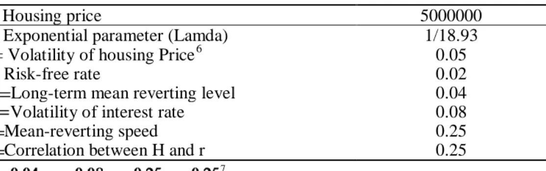
We assume the constant rate parameter of exponential distribution is 𝜆𝜆 = 1 18.93⁄ , and the homeowner’s age x equals 65.5 For the approximate pricing formula, we utilize the parameters listed below.
Simulation parameter setting table
H= Housing price 5000000
𝜆𝜆 = Exponential parameter (Lamda) 1/18.93
𝜎𝜎ℎ= Volatility of housing Price6 0.05
𝑟𝑟𝑓𝑓= Risk-free rate 0.02
Long-term mean reverting level 0.04
𝜎𝜎𝑟𝑟 =Volatility of interest rate 0.08
Mean-reverting speed 0.25
Correlation between H and r 0.25
7
Table 1 and Figure 1 illustrate the relationship between the simulations and approximations of the exponential distribution and the life table, while sigma R varies from 0.05% to 1.25%. Table 1 shows that the error of the life table increases as sigma R increases. On the other hand, the exponential distribution has a negative error at 0.05%, 0.10%, and 0.25%, while fluctuating all the way up to 1.25%. Both the exponential distribution and the life table have increasing errors while sigma R rises. Figure 1 reveals that the life table has a constant and mild increase in error from 0% to 2%, while the exponential distribution
5
Per the life table adopted, the average life expectancy of the elderly aged over 65 in Taiwan is about to be 65 + 18.94. The average life expectancy of the three distributions is set at 18.94 since average life expectancy of the exponential distribution is 18.94. The average of 18.93 might be a small error caused by rounding probability. Since the approximate formula of our research is distribution free, the estimated average and standard deviation of any countries’ future life expectancy can be applicable.
6
The parameters are taken from Buist and Yang (1998), Yang, Lin and Cho (2011), and Stephen et al. (1995). The σh value used in Stephen et al. (1995) is 0.05, 0.1 in Buist and Yang (1998), and 0.02 in Yang, Lin and Cho (2011). Therefore, we employ the median of these for our simulation parameter.
7
Regardingµr, we use the 30-year U.S. treasury rate in 2010. Chan et al. (1992), Buist and Yang (1998), Lin et al. (2006), and Yang, Lin and Cho (2011) provide values for σrof 0.08, 0.03, 0.15, and 0.15, respectively. We choose 0.08 as the volatility measure. However, because those measures are based on a CIR model, we need to convert them for the Vasicek (1977) model that we use, which results in a value of 0.01 for our simulation parameter.
Figure 1
The relationship between interest rate volatility and reverse mortgage value Table 1
Relationship between interest rate volatility and reverse mortgage value
Exponential distribution Life table
Sig_r Simulation Approximation Error Error% Simulation Approximation Error Error% 0.05% 2015101.347 2014873.055 -228.2923846 -0.01% 2158271.07 2165897.748 7626.678174 0.35% 0.10% 2018560.622 2015498.552 -3062.070112 -0.15% 2158846.329 2166269.975 7423.646628 0.34% 0.1500% 2007683.097 2017117.535 9434.437278 0.47% 2159673.269 2167271.603 7598.333724 0.35% 0.2000% 2014540.508 2019080.206 4539.697418 0.23% 2160760.023 2168215.9 7455.876758 0.35% 0.2500% 2022605.975 2020737.103 -1868.872314 -0.09% 2162115.12 2169472.164 7357.043645 0.34% 0.3000% 2018465.97 2023283.987 4818.017231 0.24% 2163747.289 2171088.961 7341.672507 0.34% 0.3500% 2017896.478 2025963.693 8067.215654 0.40% 2165665.269 2173161.365 7496.09591 0.35% 0.4000% 2016392.616 2029647.34 13254.72358 0.66% 2167877.627 2175601.553 7723.925951 0.36% 0.4500% 2029781.303 2033904.332 4123.028575 0.20% 2170392.592 2178414.25 8021.657857 0.37% 0.5000% 2012313.638 2038738.715 26425.07721 1.31% 2173217.91 2181926.262 8708.351323 0.40% 0.5500% 2037845.779 2043829.566 5983.787365 0.29% 2176360.717 2185730.95 9370.233481 0.43% 0.6000% 2028887.612 2050375.837 21488.22506 1.06% 2179827.436 2190110.996 10283.56008 0.47% 0.6500% 2033390.311 2056972.597 23582.28574 1.16% 2183623.703 2195074.626 11450.92264 0.52% 0.7000% 2048774.662 2064602.929 15828.26691 0.77% 2187754.304 2200539.174 12784.86929 0.58% 0.7500% 2041951.721 2073165.25 31213.52977 1.53% 2192223.149 2206835.888 14612.73925 0.67% 0.8000% 2058188.956 2082232.9 24043.94426 1.17% 2197033.252 2213654.293 16621.04116 0.76% 0.8500% 2046305.045 2091705.181 45400.13574 2.22% 2202186.739 2221005.882 18819.14266 0.85% 0.9000% 2068071.331 2102458.393 34387.06177 1.66% 2207684.871 2229132.221 21447.34974 0.97% 0.9500% 2072472.753 2113090.136 40617.38283 1.96% 2213528.071 2237724.608 24196.53694 1.09% 1.0000% 2072141.092 2124477.037 52335.94444 2.53% 2219715.976 2246612.348 26896.37233 1.21% 1.0500% 2100825.331 2136301.998 35476.66675 1.69% 2226247.484 2256405.112 30157.62883 1.35% 1.1000% 2097352.218 2148030.758 50678.53947 2.42% 2233120.817 2266427.529 33306.71255 1.49% 1.1500% 2093048.509 2160322.538 67274.02832 3.21% 2240333.582 2276967.843 36634.26142 1.64% 1.2000% 2090174.181 2172533.972 82359.7914 3.94% 2247882.838 2287855.029 39972.19169 1.78% 1.2500% 2094132.765 2185214.964 91082.19823 4.35% 2255765.16 2299055.266 43290.10632 1.92% -0.5% 0.0% 0.5% 1.0% 1.5% 2.0% 2.5% 3.0% 3.5% 4.0% 4.5% 5.0% Exponential Distribution Life Table Sigma R Erro r Exponential distribution Life table
fluctuates from -8% to 8%. Another trend worth pointing out is that the exponential distribution error increases violently between 1.05% and 1.25%.
Table 2 and Figure 2 illustrate the relationship between the simulations and approximations of the exponential distribution and the life table. The error percentage of the life table is roughly stable at 0.2% when LTV ranges from 0.02 to 0.34. After that, it slightly increases until 1%. The exponential distribution error percentage generally has a violent change every 4 ticks. Additionally, we also observe that the error gradually increases when LTV is larger than 0.2 up until 0.46.
Table 3 and Figure 3 illustrate the relationship between the simulations and approximations of the exponential distribution and the life table, while Sigma H varies from 0.5% to 10%. According to Table 3, the errors of the exponential distribution and the life table reach the maximum (respectively) when Sigma H is 5.5% and 6.0%. Figure 3 reveals that the life table has almost perfect correspondence among the simulations and approximations with errors stably fluctuating between -1% and 1%, whereas the exponential distribution has intensive fluctuations. After increasing along with Sigma H from 0.5% to 10%, the error percentages drop noticeably all the way down until -4.13% with a range of more than 6%. Another point we would like to emphasize is that the error is rather small under a reasonable price (mortgage value above US$2 million). If Sigma H is large, then having a minor risk premium would cause the mortgage value to be lower than the present value of US$2 million and therefore incur a larger error.
Table 4 and Figure 4 illustrate the relationship between the simulations and approximations of the exponential distribution and the life table, while the risk premium varies from 0.002 to 0.04. Figure 4revealsthat the life table has a constantly increasing error from 0% to 4%. As for the exponential distribution, the error percentages skyrocket from 2% to 4.5% and suddenly drop violently at 0.3 percent. Therefore, we can infer that 0.3 might be a critical point for the risk premium.
Table 5 and Figure 5 illustrate the relationship between the simulations and approximations of the exponential distribution and the life table, while lo varies from -0.3 to 0.3.Figure 5 reveals that the life table has a constant increase in error from 0% to 1%, while the exponential distribution’s error seesaws from -0.33%
Figure 2
Relationship between loan to value (LTV) and reverse mortgage value
Table 2
Relationship between loan to value (LTV) and reverse mortgage value
Truncated exponential distribution Life table
LTV Simulation Approximation Error Error% Simulation Approximation Error Error% 0.02 103508.014 102011.5507 -1496.463306 -1.45% 108453.2052 108675.4149 222.2097519 0.20% 0.04 205478.7902 204023.1014 -1455.688812 -0.71% 216906.4104 217350.8299 444.4195037 0.20% 0.06 307375.5228 306014.3046 -1361.218252 -0.44% 325359.6156 326023.3764 663.7608383 0.20% 0.08 409548.6494 408046.2028 -1502.446612 -0.37% 433812.8225 434701.6598 888.8372933 0.20% 0.1 515580.3247 510105.2309 -5475.093805 -1.06% 542266.0691 543379.9431 1113.873988 0.21% 0.12 616464.7537 612055.7391 -4409.014585 -0.72% 650719.6997 652046.7529 1327.053178 0.20% 0.14 718105.7114 714114.7673 -3990.944065 -0.56% 759175.3856 760759.457 1584.071488 0.21% 0.16 816950.6165 816065.2758 -885.3406842 -0.11% 867638.3763 869414.7934 1776.417106 0.20% 0.18 922451.3237 918151.4379 -4299.885802 -0.47% 976120.6582 978104.5528 1983.894634 0.20% 0.2 1032424.828 1020210.501 -12214.32669 -1.18% 1084643.666 1086782.859 2139.192736 0.20% 0.22 1131179.314 1122052.704 -9126.609694 -0.81% 1193238.809 1195461.289 2222.479798 0.19% 0.24 1237741.885 1224166.994 -13574.89104 -1.10% 1301944.597 1304117.326 2172.729538 0.17% 0.26 1337032.964 1326555.303 -10477.66117 -0.78% 1410800.224 1413004.802 2204.578744 0.16% 0.28 1441206.109 1429710.973 -11495.13694 -0.80% 1519836.465 1522012.742 2176.277226 0.14% 0.3 1546374.368 1533861.937 -12512.43023 -0.81% 1629065.37 1631310.192 2244.822007 0.14% 0.32 1645080.338 1639354.155 -5726.182948 -0.35% 1738470.384 1741303.463 2833.078922 0.16% 0.34 1753509.994 1747251.952 -6258.042183 -0.36% 1847998.271 1852203.441 4205.170328 0.23% 0.36 1854178.906 1857115.238 2936.331812 0.16% 1957553.809 1963913.178 6359.368751 0.32% 0.38 1960990.34 1969114.235 8123.894291 0.41% 2066997.692 2076670.285 9672.592782 0.47% 0.4 2058188.956 2082232.9 24043.94426 1.17% 2197033.252 2213654.293 16621.04116 0.76% 0.42 2147936.112 2193389.754 45453.64253 2.12% 2284782.389 2303585.254 18802.86494 0.82% 0.44 2259332.094 2300786.619 41454.52511 1.83% 2392647.936 2416071.137 23423.20164 0.98% 0.46 2336054.967 2401611.674 65556.7074 2.81% 2499465.464 2526484.8 27019.33631 1.08% 0.48 2431104.702 2491153.026 60048.32364 2.47% 2604940.152 2633432.162 28492.00936 1.09% 0.5 2517876.102 2568534.363 50658.26038 2.01% 2708770.282 2735781.135 27010.85244 1.00% -2.0% -1.5% -1.0% -0.5% 0.0% 0.5% 1.0% 1.5% 2.0% 2.5% 3.0% 3.5% 0.020.06 0.1 0.140.180.220.26 0.3 0.340.380.420.46 0.5 Exponential Distribution Life Table Erro r LTV Exponential distribution Life table
Figure 3
Relationship between the housing price volatility and reverse mortgage value
Table 3
Relationship between the housing price volatility and reverse mortgage value
Exponential distribution Life table
Sig_h Simulation Approximation Error Error% Simulation Approximation Error Error% 0.50% 2076109.065 2040529.444 -35579.62125 -1.71% 2182479.745 2185030.298 2550.553116 0.12% 1% 2060049.849 2040420.935 -19628.91357 -0.95% 2183482.686 2185076.201 1593.514705 0.07% 1.50% 2067709.865 2040529.625 -27180.23978 -1.31% 2184976.131 2184892.764 -83.36658104 0.00% 2% 2067075.24 2040748.382 -26326.85804 -1.27% 2186934.411 2185169.713 -1764.698475 -0.08% 2.50% 2069838.732 2042712.632 -27126.09998 -1.31% 2189216.943 2186052.707 -3164.235954 -0.14% 3% 2077858.913 2047424.158 -30434.75491 -1.46% 2191595.548 2188488.524 -3107.024077 -0.14% 3.50% 2052981.439 2055802.76 2821.32154 0.14% 2193804.357 2193276.857 -527.4996728 -0.02% 4% 2083543.454 2066722.584 -16820.86939 -0.81% 2195585.574 2199963.486 4377.911227 0.20% 4.50% 2056460.865 2076436.993 19976.12808 0.97% 2196718.729 2207492.472 10773.74328 0.49% 5% 2058188.956 2082232.9 24043.94426 1.17% 2197033.252 2213654.293 16621.04116 0.76% 5.50% 2038360.146 2081111.443 42751.29775 2.10% 2196409.379 2217167.881 20758.50216 0.95% 6% 2040385.677 2072724.601 32338.9245 1.58% 2194772.65 2217176.269 22403.61973 1.02% 6.50% 2039103.771 2057118.301 18014.53036 0.88% 2192085.853 2213452.919 21367.06571 0.97% 7% 2012488.973 2036277.693 23788.71945 1.18% 2188340.695 2206478.528 18137.83308 0.83% 7.50% 2015536.535 2011436.11 -4100.425567 -0.20% 2183550.307 2197055.987 13505.68004 0.62% 8% 2002255.019 1984174.959 -18080.06026 -0.90% 2177743.021 2185733.644 7990.622566 0.37% 8.50% 1977310.44 1955997.178 -21313.26154 -1.08% 2170957.442 2173321.272 2363.829904 0.11% 9% 1985518.71 1928546.276 -56972.4344 -2.87% 2163238.678 2160113.882 -3124.795474 -0.14% 9.50% 1971274.15 1901434.329 -69839.82155 -3.54% 2154635.541 2146533.441 -8102.100248 -0.38% 10% 1956394.675 1875602.516 -80792.15857 -4.13% 2145198.516 2132666.348 -12532.16818 -0.58% -5% -4% -3% -2% -1% 0% 1% 2% 3% Exponential Distribution Life Table Erro r Sigma H Exponential distribution Life table
Figure 4
Relationship between risk premiums and reverse mortgage value
Table 4
Relationship between risk premiums and reverse mortgage value
Exponential distribution Life table
Risk premium Simulation Approximation Error Error% Simulation Approximation Error Error% 0.002 1590253.923 1562788.325 -27465.59826 -1.73% 1412618.131 1418776.769 6158.638325 0.44% 0.004 1623532.406 1608963.782 -14568.62427 -0.90% 1472212.839 1477997.61 5784.77124 0.39% 0.006 1663620.436 1657631.42 -5989.015853 -0.36% 1534654.296 1540084.883 5430.586182 0.35% 0.008 1710399.322 1708663.69 -1735.631843 -0.10% 1600126.274 1605063.002 4936.727732 0.31% 0.01 1765971.414 1762965.686 -3005.728364 -0.17% 1668825.286 1673490.037 4664.750347 0.28% 0.012 1825130.52 1820033.56 -5096.959885 -0.28% 1740955.488 1745472.27 4516.781464 0.26% 0.014 1876093.601 1880613.351 4519.75018 0.24% 1816719.685 1821537.876 4818.191172 0.27% 0.016 1930672.768 1944313.624 13640.8561 0.71% 1896305.608 1901812.91 5507.302 0.29% 0.018 1989734.279 2011504.592 21770.31286 1.09% 1979867.026 1987010.474 7143.447824 0.36% 0.02 2058188.956 2082232.9 24043.94426 1.17% 2197033.252 2213654.293 16621.04116 0.76% 0.022 2107744.859 2156438.556 48693.6971 2.31% 2159214.866 2173180.429 13965.56255 0.65% 0.024 2185464.245 2234714.363 49250.11749 2.25% 2254907.838 2275392.631 20484.79245 0.91% 0.026 2229881.26 2315918.13 86036.86983 3.86% 2354332.7 2383448.348 29115.6482 1.24% 0.028 2294815.443 2399993.674 105178.2311 4.58% 2457079.376 2497303.93 40224.5536 1.64% 0.03 2054207.833 2057882.432 3674.599737 0.18% 2562561.982 2615825.016 53263.03428 2.08% 0.032 2043782.816 2060587.681 16804.86542 0.82% 2670020.661 2737921.535 67900.87433 2.54% 0.034 2050121.492 2063412.09 13290.59815 0.65% 2778539.611 2860922.095 82382.48379 2.96% 0.036 2045577.168 2066030.537 20453.36862 1.00% 2887081.781 2982612.07 95530.28906 3.31% 0.038 2047167.618 2069094.559 21926.94121 1.07% 2994538.295 3097939.935 103401.6398 3.45% 0.04 2050128.272 2072278.996 22150.72367 1.08% 3099788.282 3202463.106 102674.8244 3.31% -3% -2% -1% 0% 1% 2% 3% 4% 5% 0. 002 0. 004 0. 006 0. 008 0.01 0. 012 0. 014 0. 016 0. 018 0.02 0. 022 0. 024 0. 026 0. 028 0.03 0. 032 0. 034 0. 036 0. 038 0.04 Exponential Distribution Life Talbe Erro r Risk premium Exponential distribution Life table
Figure 5
Relationship between lo (ρ) and reverse mortgage value
Table 5
Relationship between lo (ρ) and reverse mortgage value
Exponential distribution Life table
lo Simulation Approximation Error Error% Simulation Approximation Error Error% -0.3 2035178.621 2036579.637 1401.016916 0.07% 2183097.856 2187396.527 4298.670949 0.20% -0.275 2022412.214 2037127.949 14715.73453 0.73% 2183613.437 2188015.642 4402.204709 0.20% -0.25 2020819.909 2037896.571 17076.66168 0.85% 2184146.203 2188776.869 4630.665716 0.21% -0.225 2030157.206 2038668.991 8511.785229 0.42% 2184695.009 2189451.182 4756.172176 0.22% -0.2 2020534.626 2039662.79 19128.16376 0.95% 2185258.776 2190222.603 4963.827413 0.23% -0.175 2047515.204 2040661.476 -6853.728051 -0.33% 2185836.479 2191137.465 5300.985818 0.24% -0.15 2035939.156 2041665.606 5726.450575 0.28% 2186427.153 2192104.406 5677.252279 0.26% -0.125 2034685.277 2043218.337 8533.059986 0.42% 2187029.887 2193032.052 6002.165294 0.27% -0.1 2040324.586 2044777.625 4453.039304 0.22% 2187643.818 2194104.382 6460.563718 0.30% -0.075 2043069.464 2046669.582 3600.117872 0.18% 2188268.134 2195321.778 7053.643165 0.32% -0.05 2032788.374 2048677.71 15889.33611 0.78% 2188902.07 2196501.026 7598.956876 0.35% -0.025 2037239.255 2050476.985 13237.73052 0.65% 2189544.9 2197780.156 8235.255418 0.38% 0 2041627.893 2052936.088 11308.19512 0.55% 2190195.945 2199021.805 8825.860591 0.40% 0.025 2034724.458 2055187.366 20462.90884 1.01% 2190854.56 2200318.065 9463.505525 0.43% 0.05 2054207.833 2057882.432 3674.599737 0.18% 2191520.139 2201806.898 10286.75867 0.47% 0.075 2043782.816 2060587.681 16804.86542 0.82% 2192192.111 2203167.298 10975.187 0.50% 0.1 2050121.492 2063412.09 13290.59815 0.65% 2192869.935 2204583.076 11713.14064 0.53% 0.125 2045577.168 2066030.537 20453.36862 1.00% 2193553.104 2205962.654 12409.54973 0.57% 0.15 2047167.618 2069094.559 21926.94121 1.07% 2194241.138 2207489.797 13248.65945 0.60% 0.175 2050128.272 2072278.996 22150.72367 1.08% 2194933.584 2209072.883 14139.29905 0.64% 0.2 2051478.129 2075584.224 24106.09508 1.18% 2195630.017 2210620.267 14990.25039 0.68% 0.225 2048126.59 2078685.04 30558.4498 1.49% 2196330.032 2212040.282 15710.25007 0.72% 0.25 2058188.956 2082232.9 24043.94426 1.17% 2197033.252 2213654.293 16621.04116 0.76% 0.275 2046895.537 2085577 38681.46311 1.89% 2197739.317 2215232.909 17493.59252 0.80% 0.3 2064593.9 2089151.713 24557.81243 1.19% 2198447.89 2216776.196 18328.30592 0.83% -0.5% 0.0% 0.5% 1.0% 1.5% 2.0% 2.5% Exponential Distribution Life Table Erro r lo Exponential distribution Life table
to 1.89%. One interesting thing from Figure 5 is that in contrast with a beautiful positive trend of the life table, the exponential distribution seems to be more active and also has a positive trend. Moreover, if we cut the figure in half when lo equals 0, then we actually can find out that the chart is similarly upside down, whereby both have a peak respectively at -0.33% and 1.89% and stably fluctuate in an absolute range of 1%.
4. Conclusion
Properly valuing reverse mortgages is an important topic, because these financial instruments are becoming increasingly common and can be an attractive cash tool for senior homeowners to use in order to improve their retirement lifestyle. Thus, the importance of valuing this significant financial instrument is growing as well.
In order to simplify the valuation of these instruments, we provide an approximation formula for valuing an annuity reverse mortgage when the housing price and interest rate are stochastic. Our approximate pricing formula greatly reduces computational intensity, because it only requires an expectation (mean) and a variance of the termination time.
We compare the results of our approximate pricing formula to the results from a Monte Carlo simulation, where the housing price and interest rate are stochastic. The analysis reveals that the difference between the results of the approximation formula and the simulation is small. To examine the robustness of our model, we use multiple commonly used distributional assumptions and find that our approximation formula is robust with respect to distributional assumptions.
References
Buist, H. and Yang, T. T. (1998). Pricing the competing risks of mortgage default and prepayment in metropolitan economies. Managerial Finance, 28(9/10), 110-128.
Boehm, T. P. and Ehrhardt, M. C. (1994). Reverse mortgages and interest rate risk. Journal of the American Real Estate and Urban Economics Association,
22(2), 387-408.
Chan, K. C., Karolyi, A., Longstaff, A. F., and Sanders, A. B. (1992). An empirical comparison of alternative models of the short-term interest rate.
Journal of Finance, 47(3), 1209-1227.
Chang, C. H., Tsai, C. C., Huang, I.-H., and Huang, H.-H. (2012). Intraday evidence on relationships among great events, herding behavior, and investors' sentiments. Chiao Da Management Review, 32(1), 61-106.
Chen, W. (2011). Market valuation of banks' loan securitizations disclosures.
Chiao Da Management Review, 31(1), 59-92.
Chi, L.-C. (2015). Does banking relationship matter in financial distress spillover?
Chiao Da Management Review, 35(1), 73-97.
Chi, L.-C. (2013). Inter-industry financial contagion and reorganization filings.
Chiao Da Management Review, 33(1), 37-63.
Harris, J. C. (1989). The effect of real rates of interest on housing prices. Journal
of Real Estate Finance and Economics, 2(1), 47-60.
Jud, G. D. and Winkler, D. T. (2002). The dynamics of metropolitan housing prices. Journal of Real Estate Research, 23(1/2), 29-45.
Kau, J. B. and Keenan, D. C. (1981). On the theory of interest rates, consumer durables, and the demand for housing. Journal of Urban Economics, 10(2), 183-200.
Klein, L. S. and Sirmans, C. F. (1994). Reverse mortgages and prepayment risk.
Journal of the American Real Estate and Urban Economics Association, 22(2),
409-431.
Lin, C. G, Chang, C. C., Yu, M., and Huang, Y. J. (2006). Valuation of Euro-convertible bonds with embedded options. Journal of Financial Studies, 14(3), 35-68.
Meen, G. (2000). Housing cycles and efficiency. Scottish Journal of Political
Economy, 47(2), 114-40.
Peiser, R. B. and Smith, L. B. (1985). Home ownership returns, tenure choice and inflation. Journal of the America Real Estate and Urban Economics
Association, 13(4), 343-360.
Reichert, A. K. (1990). The impact of interest rates, income, and employment upon regional housing prices. Journal of Real Estate Finance and Economics, 3(4), 373-391.
Stephen, W., Li, Y., Lekkas, V., Abraham, J., Calhoun, C., and Kimner, T. (1995). Conventional mortgage home price index. Journal of Housing Research, 6(3), 389-418.
Summers, L. H. (1981). Inflation, the stock market, and owner-occupied housing.
American Economic Review, Papers and Proceedings, 71(2), 429-434.
Tsay, J.-T., Lin, C.-C., Prather, L. J., and Buttimer, R. J. (2014). An approximation approach for valuing reverse mortgages. Journal of Housing
Economics, 25, 39-52.
Vasicek, O. (1977). An equilibrium characterization of the term structure.
Journal of Financial Economics, 5(2), 177-188.
Yang, T. T., Lin, C. C., and Cho, M. (2011). Collateral risk in residential
mortgage defaults. Journal of Real Estate Finance and Economics, 42(2),
115-142.
Yeh, C.-C. and Yu, H.-C. (2014). The value relevance of fair value accounting information during financial crisis. Chiao Da Management Review, 34(2), 1-26.