Magneto-optics of layers of double quantum dot molecules
L. M. Thu and O. Voskoboynikov*
Department of Electronic Engineering and Institute of Electronics, National Chiao Tung University, Hsinchu 30050, Taiwan 共Received 20 March 2009; revised manuscript received 18 August 2009; published 20 October 2009兲
We present a general treatment of the magneto-optical response from systems of semiconductor nano objects of arbitrary shapes. Our theoretical hybrid method allows us to simulate the coherent manipulation of the quantum states of electrons and holes in nano objects and monitor that by means of analysis of the collective magneto-optical response from the system. As an example of the method implementation we consider the coherent manipulation of the electronic states of a asymmetrical double InAs quantum dot molecule embedded in GaAs matrix and the collective magneto-optical properties of a layer of the molecules. Our simulation results show that changes in the quantum-mechanical configuration of the quantum dot molecules can be observable by monitoring changes in the ellipsometric data obtained for layers made from these nano objects. The ellipsometric data clearly represent the quantum mechanics of the molecules.
DOI:10.1103/PhysRevB.80.155442 PACS number共s兲: 73.21.⫺b, 75.20.Ck, 75.75.⫹a, 78.20.Bh
I. INTRODUCTION
Semiconductor nanostructured metamaterials potentially can manipulate electromagnetic fields in the optical range. The smallest building blocks of these metamaterials are made from direct-gap semiconductor’s nano objects, such as quantum dots and quantum dot molecules. At the same time those objects are expected to play an important role in de-velopment of new physics and various applications in pho-tonics as well as in electronics and solid-state quantum memory.1,2 Progress in modern semiconductor technologies has allowed us to experimentally and theoretically model the various semiconductor nanostructures within a wide range of geometries and material parameters. For instance, it is pos-sible to fabricate vertically stacked quantum dots 关quantum dot molecules 共QDMs兲兴 of high quality and uniformity.3–5 The quantum-mechanical coherent coupling and forming of molecular states in the stacked quantum dots can be consid-ered in complete analogy to real molecules. But in contrast to the real molecules the artificial design of semiconductor QDMs provides us with the unique opportunity to dynami-cally manipulate and reconfigure wave functions of electrons and holes confined in QDM 共see, for instance, Refs. 6–15 and references therein兲. QDMs have attracted much interest because they are very likeable candidates for the implemen-tation of quantum bits.2 From the other side, proper under-standing of the connection between the electronic-state co-herent coupling in isolated nano objects and the collective electromagnetic response of layers assembled from them16is a prerequisite to make new nanostructured metamaterials, with on-demand properties not resembling anything in nature.17–23We should conclude that the future development of the quantum informatics and metamaterial’s quantum op-tics both require for an extensive investigation of the collec-tive response of ensembles of semiconductor QDMs.
In order to reach those goals in this theoretical study we formulate a computational method which allows us to moni-tor the coherent manipulation of the quantum states of elec-trons and holes in embedded semiconductor nano objects by means of the magnetoellipsometry. The influence of the sur-rounding semiconducting matrix on the polarizability of the
nano objects has been imposed using a generalization of the hybrid discrete-continuum model.16,24,25 The generalization allows us to simulate the nano objects of arbitrary shapes. We show that parameters of the electron and hole quantum states localized in the nano objects can be retrieved from the collective magneto-optical response of systems of such nano objects. As an example of the method implementation we consider impact of the coherent manipulation of electronic states in the double vertical lens-shaped circular QDM on the collective magneto-optical response from a layer of those nano objects. The manipulation is performed by an external magnetic field applied upon InAs/GaAs quantum dot mol-ecules assembled from the dots with substantially different lateral radii. Recently it was demonstrated that in the asym-metrical QDM the nonuniform diamagnetic shifts of the low-est electron-energy levels lead to their anticrossing which yields in a positive peak of the differential magnetic suscep-tibility of the system.26 In this paper we show unusual con-sequences of the nonuniform diamagnetic shifts for the magneto-optics of layers of asymmetrical QDMs. We treat the semiconductor QDMs within complete three-dimensional description which allows us to simulate arbitrary directions of the external magnetic field共Fig.1.兲 in contrast to most of the calculations done before. It brings up much wider oppor-tunities to dynamically manipulate electron and hole states in QDMs. As it was already mentioned changes in
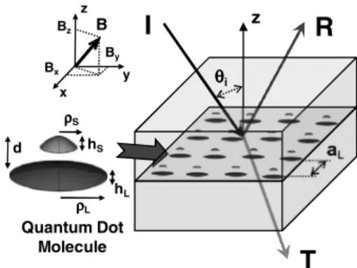
magneto-B x y z Bz Bx By Quantum Dot Molecule ρρρρS ρρρρL d hS hL aL
I
R
T
z θθθθiFIG. 1. Schematic of the magneto-optics of a layer of embedded semiconductor quantum dot molecules.
optical response of a layer of QDMs emerge from the changes in the quantum-mechanical configuration of the QDMs. In this paper we demonstrate in detail that the mag-netoellipsometric data can reproduce an important and clear information on the quantum mechanics of the molecules.
II. THEORY
A. Hybrid model and discrete dipole approximation In order to make this paper more self-contained, we will repeat and reformulate some of the aspects of the theory presented in Refs. 16, 24, and 25. We consider a system 共layer兲 of QDMs of characteristic size a embedded into a semiconductor host matrix, which is transparent for the in-coming共external兲 light beam 共Fig.1兲. For such a system we assumeⰇaL⬎a, where is the wavelength of the
electro-magnetic wave and aL is an average distance between
QDMs. It has been shown in Ref. 24 that under those as-sumptions we can use the hybrid model to describe the op-tical response of the system by means of polarizabilities of discrete dipoles embedded into the continues dielectric ma-trix. All the dipoles are assigned to the xy plane. The incom-ing light beam has a simple plane-wave character
EX共r兲 = E0eikmr,
km=
冑
⑀mk, 共1兲k =共k储,kz兲 = 共kx,ky,kz兲, 共2兲
where⑀mstands for the dielectric constant of the host matrix, k =/c is the vacuum wave vector, andrepresents the light frequency.
In the linear discrete dipole approximation 共DDA兲 共see Refs. 27and 28, and references therein兲 the QDM’s excess dipole strength p follows from Ref.24
p =
冕
QDM
dr3关P共r兲 − P
m共r兲兴, 共3兲
where P共r兲 is the polarization density inside the QDM with the dielectric constant ⑀QDM and Pm共r兲 is one of the host
matrix with the dielectric constant ⑀m. The embedded bare
polarizability␣JEBis defined with respect to the internal
ap-plied electric field EA关a spatial average of the internal to the
QDM microscopic electric field e共r兲兴 by
p =␣JEBEA. 共4兲
Within the electromagnetic nonlocal discrete description
EA= EL+ tJp, 共5兲
where EL is the classical local field, which is equal to the
external plane-wave field EX in the case of a single QDM,
and tJ is the full electromagnetic self-interaction tensor for the QDM. The bare polarizability can be obtained by means of theory.16,29
The embedded dressed polarizability␣JEDrefers to
experi-mental observations and it is defined by
p =␣JEDEL. 共6兲
The elementary relationship between those two kinds of po-larizability can be written as
␣
JEB−1−␣JED−1 = tJ. 共7兲
For our system of embedded QDMs in the linear DDA we can write the local field at the position riof the ith dipole as
ELi= EXi+
1
⑀m
兺
j⫽ifJijpj, 共8兲
EXi= EX共ri兲, 共9兲
where fJij is the vacuum intercellular 共interdipole兲 transfer
tensor关the dyadic Green’s function in the DDA共Ref.27兲兴
fJij= fJ共ri− rj兲 = exp共ikm⌬rij兲 4⑀0⌬rij ⫻
冋
km 2共IJ− ⌬rˆ ij⌬rˆij T兲 −1 − ikm⌬rij ⌬rij2 共IJ− 3⌬rˆij⌬rˆij T兲册
, ⌬rij= ri− rj, ⌬rˆij= ⌬rij ⌬rijand IJ is the identity dyadic. The induction for the excess dipole strength’s pibecomes
pi=␣JEDi
冉
EXi+1
⑀m
兺
j⫽ifJijpj
冊
. 共10兲From Eq. 共10兲 we obtain the system of equations to be solved
兺
j TJijpj= EXi, 共11兲 where TJij=␦ij共␣JEBi −1 − tJi兲 + 共1 −␦ij兲fJij, t Ji= tJi S + i 3 6⑀m⑀03 I J, t JiSis the static part of the self-interaction tensor to which we have added the Lorentz radiation damping共the term with3 above兲.
The collective optical response of the system is character-ized by the reflection and transmission coefficients. They have to be obtained from the far-field expression of the re-mote dipole field at a point r far from the layer location. Using solutions of Eq. 共11兲 we get, for the reflection and transmission, respectively, ER共r兲 =
兺
i F Ji共r兲pi, when z→ + ⬁; ET共r兲 = EX共r兲 +兺
i F Ji共r兲pi, when z→ − ⬁, 共12兲 whereF Ji共r兲 =exp共ikm⌬ri兲 4⑀0⑀m⌬ri km 2共IJ− ⌬rˆ i⌬rˆi T兲, ⌬ri= r − ri.
After Eq. 共12兲 it is trivial to calculate the transmission and reflection coefficients of the layer. The formulation of the systems 共11兲 and 共12兲, in general, traces a method of simu-lation of the optical response from an arbitrary system of semiconductor nano objects embedded into semiconductor host materials. The larger the tensor matrix TJij, the more
interesting problems may be studied. But therefore 共if we would like to consider three-dimensional random arrays of semiconductor nano objects兲 the calculation of the matrix elements of TJijrequired and solution of Eq.共11兲 are already
tedious problems themselves. So, in this paper we confine ourselves to a single layer共two-dimensional array兲 of QDMs embedded the semiconductor host matrix共Fig.1兲
In the case of a two-dimensional square lattice of QDMs of the lattice parameter aL the calculation of the optical
re-sponse of the embedded layer can be performed on the base of the Vlieger’s expression30,31
ER共r兲 = FJ共r兲pef, 共13兲 where F J共r兲 = ikm2e ikmr 2⑀0⑀maL2kmz 共IJ− ⌬kˆm⌬kˆm T兲
is the Vlieger’s remote interplanar transfer tensor, km= k储
− kzzˆ and the effective dipole pef induced in the layer is
ob-tained from pef=关IJ−␣JEBfJ兴−1␣JEBE0, fJ = fJ S 4⑀0⑀maL3 + tJS+i共km 2J − ⌬kI 储m⌬k储m T − kmz2 zˆzˆT兲 2⑀0⑀maL2kmz , 共14兲 fxxS = fyy S = −fzz S 2 = − 4.51681. 共15兲
Using the Vlieger’s approach we can determine the reflection 共rss, rpp兲 and transmission 共tss, tpp兲 coefficients, and
absor-bance 共Ass, App兲 of the layer. For a two-dimensional array
共square lattice兲 of the dipoles, the coefficients are given by30,31 rss= f Aycosi− f , rpp= f cosi Ax− f cosi − f sin 2 i Azcosi− f sin2i , tss= 1 + rss, tpp= f cosi Ax− f cosi − Azcosi Azcosi− f sin2i , Ass共pp兲= 1 −兩rss共pp兲兩2−兩tss共pp兲兩2. 共16兲
Here subscribers “s” and “p” refer to the light polarization perpendicular and parallel to the plane of incidence, respec-tively,iis angle of incidence
A= 4⑀0aL 3共␣ EB −1 − t兲 −f S ⑀m , f = 2iaLkm.
The ellipsometric angles ⌿ and ⌬ represent the experi-mental values and can be measured with the highest accu-racy. They follow from a conventional definition
rpp rss
= tan⌿ei⌬ and also can be calculated numerically.
B. Polarizability and quantum mechanics of QDMs The hybrid discrete-continuum method allows us to simu-late the collective electromagnetic response of the layer of embedded QDMs.24,25The embedded bare polarizability␣J
EB
of a single QDM approximated at the near resonance condi-tions can be written as16,22,24,29,32–34
␣JEB共兲 =␣JEB S
+␣JD共兲, 共17兲
where ␣JEB S
is the static part of the polarizability35,36 of the QDM共to be treated later兲 and
␣JD共兲 =e 2 ប
兺
n rnⴱrn T fn共兲 共18兲is the dynamic part of the polarizability. In the equations above: rn stands for the optical transition-matrix
element16,29,37 fn共兲 =
冉
En ប冊
冋
1 n−− i⌫n册
共19兲 is the frequency-dependent function introduced in Refs. 16 and29, which depends on transition energies En=បnof theresonance optical transitions of the QDM and corresponding damping factors⌫n, e is the elementary charge. Faraday/Kerr
or Cotton/Mouton-type magneto-optical effects are not taken into account here.
To find the static part of the polarizability tensor␣JEB S
we implement the following boundary-value problem for a local electrostatic potential ⌽共r兲 in a complex three-dimensional cubic domain of the host material including one QDM共Refs. 35and36兲
ⵜr关⑀共r兲ⵜr⌽共r兲兴 = 0,
− L⬍⬍ L, =兵x,y,z其, 共20兲 where
⑀共r兲 =
再
⑀QDM, when r is inside QDM⑀m, when r is outside QDM
冎
.
An isolated QDM is located in the center of the domain and
LⰇa. We solve the problem 共20兲 in conjunction with three
sets of the boundary conditions
sx
再
⌽共r兲兩−L,y,z=⌽共r兲兩x,⫾L,z=⌽共r兲兩x,y,⫾L= 0 ⌽共r兲兩+L,y,z= 2LE0冎
, sy再
⌽共r兲兩x,−L,z=⌽共r兲兩⫾L,y,,z=⌽共r兲兩x,y,⫾L= 0 ⌽共r兲兩x,+L,z= 2LE0冎
, sz再
⌽共r兲兩x,y,−L=⌽共r兲兩⫾L,y,z=⌽共r兲兩x,⫾L,z= 0 ⌽共r兲兩x,y,+L= 2LE0冎
. 共21兲 The solutions give us the space distribution of the electric field E共r兲=−⌽共r兲 and polarization density P共r兲=⑀0关⑀共r兲− 1兴E共r兲 when the external uniform electric field E0 is par-allel to xˆ, yˆ, or zˆ correspondingly. Following the scheme described above the static parts of the embedded bare polar-izability, embedded dressed polarizability, and self-interaction tensor can easily be obtained according to Eqs. 共4兲, 共6兲, and 共7兲 for the appropriate s
␣EB S = d E ˜ , ␣ED S = d E0, tS =共␣EB S 兲−1−共␣ ED S 兲−1, 共22兲 where E˜ =1 V
冕
QDMdr 3E共r兲and V is the QDM volume.
For the dynamic part of the polarizability we have to com-pute the transition energies and wave functions of electrons and holes confined in the asymmetrical InAs/GaAs QDM. In our calculations we use a three-dimensional hard-wall con-finement potential and realistic semiconductor material pa-rameters 共for instance, the band offset of the InAs/GaAs strained heterostructure, corrected to the strain conditions band parameters, etc.兲. The electron states are described by means of the effective one-band Hamiltonian,16,38,39 which can properly describe the strong nonparabolicity in the InAs conduction band39–41 Hˆe=
冋
⌸ˆe 1 2me共E,r兲 ⌸ˆe+ Ve共r兲册
I2+ B 2 ge共E,r兲· B, 共23兲 where: I2 is the identity matrix of size 2, ⌸ˆe= −iបⵜr + eA共r兲 is the momentum operator for electrons, ⵜr is the spatial gradient, A共r兲=12共B⫻r兲 is the vector potential for the
uniform arbitrary directed magnetic field B =共Bx, By, Bz兲,
me共E,r兲 is the energy and position-dependent electron
effec-tive mass 1 me共E,r兲 = 2P 2 3ប2
冋
1 E + Eg共r兲 − V共r兲 + 1 E + Eg共r兲 − V共r兲 + 2⌬共r兲册
共24兲 and ge共E,r兲 = 2再
1 − m0 me共E,r兲 ⌬共r兲 3关E + Eg共r兲兴 + 2⌬共r兲冎
共25兲 is the electronic Landé factor. In the equations above: Eg共r兲and⌬共r兲 stand for the position-dependent band gap and spin-orbit splitting in the valence band, P is the momentum ma-trix element,38,42 is the vector of the Pauli matrices,
B is
the Bohr magneton, m0is the free-electron mass, and Ve共r兲 is
the hard-wall confinement potential for electron
Ve共r兲 =
再
0, when r is inside QDM
Ve 0
, when r is outside QDM
冎
, 共26兲 where Ve0 is the conduction-band offset in the InAs/GaAsquantum dot.
For the proper description of the valence-band 共hole兲 states in InAs/GaAs quantum dots we should consider multi-band k · p Hamiltonian that allow for valence submulti-band mix-ing共see, for instance, Refs.14and43–46兲. For the transition frequencies being almost at the edge of the gap of the QDM material the heavy-light hole mixing should be included and the low-energy hole states can be described by the four-band Luttinger-Kohn Hamiltonian14,40,41,46,47 Hˆh= 1 2m0
冢
Pˆ+ Rˆ − Sˆ 0 Rˆⴱ Pˆ− 0 Sˆ − Sˆⴱ 0 Pˆ− Rˆ 0 Sˆⴱ Rˆⴱ Pˆ +冣
+ Vh共r兲I4, 共27兲 where Pˆ⫾=关共␥1⫾␥2兲⌸ˆh⬜ 2 +共␥1⫿ 2␥2兲⌸ˆhz 2兴, Rˆ = −冑
3␥2⌸ˆh− 2 , Sˆ = 2冑
3␥3⌸ˆh−⌸ˆhz.In the above expressions: I4 is the identity matrix of size 4, 兵␥1,␥2,␥3其 is a set of the Luttinger parameters, the
momen-tum operators⌸ˆh are defined as the following:
⌸ˆh= − iបⵜr− eA共r兲, ⌸ˆh⬜ 2 =⌸ˆhx 2 +⌸ˆhy 2 , ⌸ˆh⫾=⌸ˆhx⫾ i⌸ˆhy
Vh共r兲 =
再
0, when r is inside QDM
Vh 0
, when r is outside QDM
冎
, 共28兲 where Vh0is the valence-band offset in the InAs/GaAsquan-tum dot.
For an electronic state confined in the QDM the wave function is presented by the two component spinor
Fel兵2其共r兲 =
再
Fel↑共r兲兩S典兩↑典 Fel↓共r兲兩S典兩↓典
冎
, 共29兲
where l stands for the main quantum number,=↑ ,↓ refers to the spin polarization and 兩S典 is a spherically symmetric Bloch function.41,42 The envelop wave functions F
el 共r兲
should satisfy the Schrödinger equation
Hˆe
再
Fel↑共r兲 Fel↓共r兲冎
= Eel再
Fel↑共r兲 Fel↓共r兲冎
. 共30兲A confined hole state with the main quantum number k can be written as a four-component Luttinger spinor14,42,47
FhkJ兵4其共r兲 =
冦
Fhk+3/2共r兲冏
3 2,+ 3 2冔
Fhk−1/2共r兲冏
3 2,− 1 2冔
Fhk +1/2共r兲冏
3 2,+ 1 2冔
Fhk−3/2共r兲冏
3 2,− 3 2冔
冧
, 共31兲where 兵兩32, +32典,兩32, −12典,兩32, +12典,兩32, −32典其 is the conventional Luttinger-Kohn basis.16,41,42,47 The envelop functions F
hk Jz共r兲
are the components of the hole’s eigenfunction of the Hamil-tonian 共27兲 Hˆh
冦
Fhk +3/2,共r兲 Fhk−1/2,共r兲 Fhk+1/2,共r兲 Fhk −3/2,共r兲冧
= Ehk冦
Fhk +3/2,共r兲 Fhk−1/2,共r兲 Fhk+1/2,共r兲 Fhk −3/2,共r兲冧
. 共32兲The above hole states are designated by the main quantum number k and their chirality v =⇑ ,⇓. The hole’s chirality is
isomorphic to the electronic spin-quantum number: states with opposite chirality are orthogonal and they are degener-ate in the absence of magnetic field.14,15,48,49We use the com-puted electron and hole wave functions and energies to simu-late the dynamic part of the polarizability tensor in Eq.共17兲.
III. NUMERICAL RESULTS AND DISCUSSION Now we apply the strategy developed above to the case of a layer of double vertical lens-shaped circular quantum dot molecules. To do this we use realistic semiconductor material parameters and dimensions of the dots in the molecule known in literature.15,42,45,50,51Our molecule consists of two quantum dots with substantially different radii L⬎S and
heights hL⬍hS 共the subscripts L and S indicate “large” and
“small” dots in Fig. 1兲. So, the QDM is nonuniform in z direction. All calculations were performed for the molecule with the following geometry parameters:5,26
L= 25 nm, S
= 9.5 nm, hL= 3 nm, hS= 4 nm, and a few interdot
共base-to-base兲 distances d.
The static parts of the polarizability tensors of the QDM was calculated with the approach described above using
COMSOLmultiphysics package.52The dielectric constants are taken like the following: ⑀QDM=⑀InAs= 15.2 for the inside
InAs material andm=GaAs= 13.1 for the GaAs matrix. Note
that due to the cylindrical symmetry of the QDM, the static parts of polarizability tensors are diagonal and ␣xx
S =␣yy S ⫽␣zz S 共so, t xx S = tyy S ⫽t zz
S as well兲. The corresponding
normal-ized results for a system with the two-dimensional lattice parameter aL= 100 nm and interdot distance d = 10 nm are
given in TableI as an example. The results are used in our calculations of the magneto-optical response from the layer of QDMs.
In the first place we simulate the embedded bare polariz-ability␣JEB共兲 共and the magneto-optical response of the
sys-tem兲 without excitonic effects 共we ignore interaction be-tween electrons and holes in optical transitions兲. Some excitonic effects in the QDMs are discussed in Appendix. For the noninteracting electrons and holes ␣JD共兲 can be
written as the following:16,29
␣JD共兲 =e 2 បl,;J
兺
z,k, reⴱ;Jz,hre;Jz,h T 兩具F hk Jz,兩F el 典兩2f k,l共兲, fk,l共兲 =冉
Ek,l ប冊
冋
1 k,l−− i⌫k,l册
, 共33兲where reh stands for the bulk interband optical matrix
element,16,37 ប
k,l= Ek,l= Ehk+ Eel+ Eg present
transi-tion energies of the resonance optical transitransi-tions from hole energy levels 共hk兲 to electron energy levels 共el兲 of the QDM, and⌫k,lstand for the corresponding damping factors
共Eg is the energy gap of the dot’s semiconductor material兲.
The hole-electron overlap integrals具Fhk Jz,兩F
el
典 should be
cal-culated using the envelop functions Fel共J共hk兲z
,兲 from Eqs. 共30兲
and共32兲.
To model the optical transition energies and overlap inte-grals we determine material parameters for the InAs/GaAs quantum dot molecule. According to the data from Refs.14, 26,44,45,50, and51we choose for the strained InAs inside the dot: EgInAs= 0.842 eV, ⌬InAs= 0.39 eV, meInAs共0兲
= 0.044 m0,␥1InAs= 11.65,␥2InAs= 3.86, and␥3InAs= 3.87. For
the GaAs surrounding matrix: EgGaAs= 1.52 eV, ⌬GaAs = 0.341 eV, meGaAs共0兲=0.067 m0, ␥1GaAs= 6.98, ␥2GaAs TABLE I. Components of the static parts of embedded polariz-abilities␣JEB共D兲and self-interaction tensor tJ of InAs/GaAs QDMs 共␣0= 4⑀0aL 3 = 11.127⫻10−32 Fm2兲. ␣EB S ␣ ED S tS ␣xx共yy兲 5.167⫻10−4␣0 5.119⫻10−4␣0 −18.148⫻␣0 −1 ␣zz 1.050⫻10−4␣0 0.923⫻10−4␣0 −1310.430⫻␣0 −1
= 2.06, and ␥3GaAs= 2.93. Using these parameters, the band offsets of conduction band and valence band can be found as:
Ve0= 0.474 eV and Vh0= 0.203 eV. The energies and wave
functions of electrons and holes confined in the QDM are obtained numerically form solutions of Eqs.共30兲 and 共32兲 by the nonlinear iterative method53 using the COMSOL mult-iphysics package.52
Now we present the transition energies and overlap inte-grals of noninteracting electrons and holes共excitonic effects are discussed in Appendix兲. We consider three distances be-tween dots in the QDM: d1= 20 nm, d2= 10 nm, d3= 5 nm,
and three directions of the magnetic field: B关1兴=共0,0,Bzˆ兲,
B关2兴=冑12共0,Byˆ,Bzˆ兲, B关3兴=共0,Byˆ,0兲. For the reason of clarity
we concentrate on the optical transitions between four lowest hole energy states h1共2兲 共=⇑ ,⇓兲 and four lowest elec-tronic states e1共2兲 共=↑ ,↓兲 under the condition of the spin-chirality alignment in the transition. In our general con-sideration the magnetic field is not parallel to the system growth direction zˆ. This does not allow us to use any simple specific selection rules for the interband optical transitions. Now we should impose the following rule: certain transition is allowed when the corresponding three-dimensional over-lap integral cannot be vanished.
For configurations 兵di, B关j兴其 共i, j=1,2,3兲 the lowest
tran-sition energies and corresponding overlap integrals are
shown in Figs.2–7. It should be noted that according to our simulation experience 共see also Ref. 46兲 the predominant components of the Luttinger spinor FhkJ兵4其z are those of Jz
=⫾32 for all involved hole states and the system’s configu-rations. The components of Jz=⫾
1
2 always give small
corre-sponding contributions in this energy range. Therefore, for the optical transitions being considered Jz=⫾
3
2 components
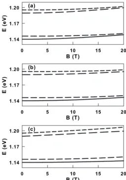
FIG. 2. Transition energies for d = d1as functions of magnetic field at different directions of the magnetic field. Inset: the anti-crossing region. B (T) 0 5 10 15 20 0.0 0.5 1.0 B (T) 0 5 10 15 20 0.0 0.5 1.0 B (T) 0 5 10 15 20 0.0 0.5 1.0 (a) (b) (c) 10.6 10.7 10.8 0.0 0.5 1.0
FIG. 3. Overlap integrals共squared absolute values兲 as functions of magnetic field for d = d1and different directions of the magnetic field关descriptions of the transitions see in Fig.2共a兲兴.
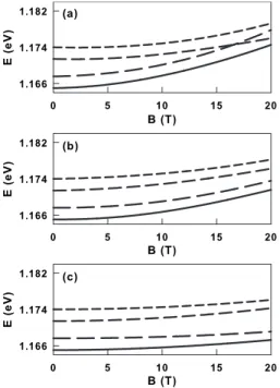
FIG. 4. Transition energies for d = d3as functions of magnetic field at different directions of the magnetic field关descriptions of the transitions see in Fig.2共a兲兴.
give the predominant共95%兲 contributions to the sum of the squared overlap integrals in the dynamic part of the polariz-ability关see Eq. 共33兲兴. Using this result in Figs.3,5, and7we present only the squared absolute value of 具Fhk
+3/2,⇑兩F el ↑典.54 The first crucial difference between results for two dis-tances d1 and d3 when B = B关1兴 is the anticrossing of the
electronic energies. For the large distance between dots 共d1兲 the tunnel coupling between them is weak. The
nonunifor-mity of the QDM geometry in z direction generates the non-uniform diamagnetic shifts of the electron energies26 which leads to the anticrossing for e1 and e2 states at B1AC
⬇10.7 T. The anticrossing was discovered and discussed in details in Ref. 26. At the same time energy levels for holes do not anticross within this range of the magnetic field. This leads to the anticrossing for the energies of h1→e1 and
h1→e2 transitions 关see inset of Fig. 2共a兲兴. Here we should stress that the anticrossing manifests redistribution of the electronic wave function inside the QDM: the electronic wave function of the state e1 at B1AC relocates from the
large dot to the small one. On the contrary, the second state
e2 relocates from the small dot to the large one. At the same time, the probability density of the hole state h1 re-mains to localize in the large dot and the probability density of the hole state h2—in the small dot. This leads to the steplike behavior of the corresponding overlap integrals at
B = B1AC关see Fig.3共a兲兴. Clearly, when the distance between
the dots in the QDM is large, the magnetic field can drasti-cally change the overlap integrals for the corresponding op-tical transitions as it is shown in Fig.3共a兲. The nonuniform diamagnetic shift also produces crossings between h1
→e2 and h2→e1 transition energies at B1C⬇18.3 T
关Fig. 2共a兲兴. But this crossing appears without relocations of the electron wave functions and it has no impact on the over-lap integrals. The small distance共d3兲 and strong tunnel
cou-pling between dots lead to the strong hybridization between electronic states e1 and e2.26,55 This creates molecular states for electrons with symmetric and antisymmetric con-figurations along z direction.14,26,55 The diamagnetic shifts 共when B=B关1兴兲 become uniform and no anticrossings 共wave
function’s redistributions兲 or crossings appear 关see Figs.4共a兲 and5共a兲兴. B (T) 0 5 10 15 20 0.0 0.5 1.0 B (T) 0 5 10 15 20 0.0 0.5 1.0 B (T) 0 5 10 15 20 0.0 0.5 1.0 (a) (b) (c)
FIG. 5. Overlap integrals共squared absolute values兲 as functions of magnetic field for d = d3and different directions of the magnetic field关descriptions of the transitions see in Fig.2共a兲兴.
FIG. 6. Transition energies for d = d2as functions of magnetic field at different directions of the magnetic field关descriptions of the transitions see in Fig.2共a兲兴.
B (T) 0 5 10 15 20 0.0 0.5 1.0 B (T) 0 5 10 15 20 0.0 0.5 1.0 B (T) 0 5 10 15 20 0.0 0.5 1.0 (a) (b) (c)
FIG. 7. Overlap integrals共squared absolute values兲 as functions of magnetic field for d = d2and different directions of the magnetic
The system with the distance d2 共B=B关1兴兲 presents an intermediate case when the anticrossing and hybridization coincide. This is the reason why a weak convergence of the energies for the transitions h1→e1 and h1→e2 and some typical changes in the overlap integrals can be seen in Figs. 6共a兲 and7共a兲. Yet, the energy crossing for the transi-tions h1→e2 and h2→e1 remains at B1C⬇16.6 T.
To complete the picture of the interplay between of the distance and magnetic field impacts on the transition energies and overlap integrals, we show Ekl共B兲 and 兩具Fhk
+3/2,⇑兩F el ↑典兩2for
few directions of the magnetic field in Figs. 2–7. For the large distance between dots within the QDM共d1兲 the change
in the magnetic field direction from B关1兴 to B关2兴 leads to a shift of the anticrossing 共crossing兲 point according to the obvious scaling rule关Fig.2共b兲兴
B2AC⬇
冑
2B1AC,B2C⬇
冑
2B1C关note: B2C⬇25.9 T and the crossing is located out of the
range of Fig.2共b兲兴. At the same time the overlap integrals at the anticrossing for the allowed transitions demonstrate some deviations from the pure steplike behavior. Figure 3共b兲 pre-sents a typical manifestation of the changes in the electron and hole wave function’s distributions between two dots. Again the decrease in the distance between dots removes the traces of the anticrossing and the wave function’s relocation 关Figs.4共b兲,5共b兲,6共b兲, and7共b兲兴. When the magnetic field is parallel to xy plane共B关3兴configuration兲 the anticrossing and crossing have disappeared even for d = d1. The overlap
inte-grals being functions on the magnitude of the magnetic field simply reflect changes in the confinement of the electron and hole wave functions along z direction in different dots. The electron states confined in high共small兲 dot are more sensitive to the magnetic field. The electron wave functions localized in the large dot are obviously under strong confinement in z direction already for B = 0 and hardly can be squeezed more by the magnetic field applied along y direction. At the same time the sensitivity of the hole wave functions to the mag-netic field is much weaker, no mater in which dot the func-tion is localized. The reducfunc-tion in the interdot distance con-ventionally hybridizes electron states from different dots. This finally forms a typical “molecular” magnetic properties of the QDM as it is shown in Figs.4共c兲and5共c兲.
Using the above discussed quantum-mechanical proper-ties of the transition energies and overlap integrals we inves-tigate now the collective magneto-optical response of the layer of QDMs with the two-dimensional lattice parameter
aL= 100 nm. First we combine all our data on the static parts
of the polarizability tensors with the results of the quantum-mechanical calculations into the complete ␣JEB共兲 using reh
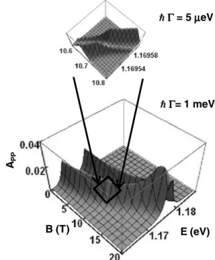
= 0.6 nm.16,37 Obviously, small damping parameter ⌫ en-sures a clear reflection of the quantum-mechanical properties of an individual QDM in the collective magneto-optical re-sponse of the layer of QDMs. At the same time in our theory ⌫ has to be used as a free parameter.16,29 To demonstrate importance of the parameter value we present in Fig. 8 the absorbance of the layer of the QDMs in兵d1; B关1兴其
configura-tion for the incidence of i= 60°. The inset of Fig.8gives a
filling of the impact of the parameter on the observation of the energy gap at the anticrossing of the transition energies when ⌫ is small 关see Inset of Fig. 2共a兲兴. The peak in Fig.8 corresponds to the crossing of the two transition energies
h1→e2and h2→e1in Fig.2共a兲. In the crossing point they contribute in resonance simultaneously and this in-creases the response by the factor of 2. We should stress, that even for relatively largeប⌫=1 meV the quantum mechanics of the QDM clearly shows itself from the magneto-optical data. So, we will setប⌫=1 meV for all calculations below. Note, we present here only peaks corresponding to the tran-sitions considered in Figs.2–7. Our calculation results show that we always can distinguish them ifប⌫ⱕ1 meV.16,24,25,55 The ellipsometric angles ⌿ and ⌬ can be measured with the highest accuracy. The direct accessibility of the quantum information from the QDMs such as individual dipole strengths, transition energies, and overlap integrals by means of the measurement of the ellipsometric parameters is one of the attractive aspects of our approach.
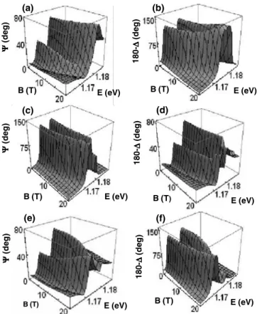
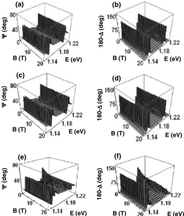
In order to illustrate that we show in Figs. 9–11relevant data on the magnetoellipsometry of a layer of InAs/GaAs QDMs for the incidence of i= 60°. For the ellipsometric
angle⌿ the results systematically reproduce the transforma-tion of the quantum-mechanical properties of the individual QDMs when we change the system configuration from 兵d1, B关1兴其 关Fig.9共a兲兴 to 兵d3, B关3兴其 关Fig.11共f兲兴. The variation in
the magnetic field magnitude makes the transformation even more clear and understandable. At the first glance the anti-crossing features of the transition energies and overlap inte-grals are not clear in Figs. 9共a兲and 9共b兲 for 兵d1, B关1兴其
con-figuration whenប⌫=1 meV 共note, we can see them clearly if ប⌫=1 eV兲. Yet, the crossing as another result of the nonuniform diamagnetic shift 共pure quantum-mechanical
E (eV) B (T)
APP
Ñ ΓΓΓΓ= 1 meV Ñ ΓΓΓΓ = 5 µµµµeV
FIG. 8. Absorbance for a monolayer of InAs/GaAS QDMs in 兵d1, B关1兴其 configuration.
phenomenon兲 obviously shows itself as a combined peak in Figs. 9共b兲 and 10共b兲. In general the transformations of the overlap integrals共connected to the changes in electron wave-function localization兲 can be easily recognized in Figs.9and 10. Therefore we can say that, when the distance between dots in the QDM is large enough, the magnetic field acts as a dynamic coupling factor for electron energy states localized in different dots on the analogy of the interdot distance in the static approach. At the same time for the interdot distance d3
the ellipsometry simply exhibits the conventional molecular diamagnetic shift for all directions of the magnetic field共Fig. 11兲. For all configurations the variation in both ellipsometric angles is clearly within the range of any modern ellipsometer56 which gives us an opportunity to monitor op-tically coherent dynamic 共when B is changing兲 and static 共when d is changed兲 transformations and tuning of the elec-tron wave functions in QDMs.
IV. CONCLUSION
For systems of semiconductor embedded nano objects of arbitrary shapes we have formulated a modification of the hybrid discrete dipole approximation. The modification al-lows us to describe the collective magneto-optical response of systems of such objects. As an example of the theory implementation we have performed a comparative study of the magneto-optical response functions共absorbance and the ellipsometric angles兲 for a layer of asymmetrical InAs quan-tum dot molecules arranged in a square two-dimensional
lat-tice and embedded into GaAs matrix. The response of indi-vidual embedded QDMs is presented in terms of the excess polarizability. Static and dynamic parts of the polarizability 共and the self-interaction tensor as well兲 are determined. Us-ing the Veliger’s derivation we simulated the ellipsometric angles of the layer embedded QDMs for a wide range of the system configuration. We emphasize that the magnetoellipso-metric data reproduce important information on the quantum mechanics of the molecules. Varying magnetic field and the distance between quantum dots within the layer we can in-vestigate optically the transition from molecular to “atomic” behavior of the system. This general conclusion remains valid when excitonic effects are taken into consideration. Our simulation results clearly suggest measurable values for the ellipsometric data for any modern ellipsometric setup. The approach can be potentially useful for simulation and characterization of new all-semiconductor nanostructured metamaterials.
ACKNOWLEDGMENTS
We thank Shao-Fu Xue for assistance in the calculations. O.V. thanks V. Ryzhii for his hospitality at the University of Aizu 共Japan兲 where a part of the paper was written. This work is supported by the National Science Council of the Republic of China under Contracts No. NSC 97-2112-M-009-012-MY3, No. NSC 97-2120-M-009-004, and No. NSC 98-2918-I-009-001, and by the Ministry of Education of
Tai- 180-∆∆∆∆ (de g ) ΨΨΨΨ (de g ) 180-∆∆∆∆ (de g ) 180-∆∆∆∆ (de g ) ΨΨΨΨ (de g ) ΨΨΨΨ (de g ) B (T) B (T) B (T) B (T) B (T) B (T) E (eV) E (eV) E (eV) E (eV) E (eV) E (eV) (a) (b) (c) (d) (e) (f)
FIG. 9. Ellipsometric angles for d = d1and different directions of
the magnetic field:关共a兲 and 共b兲兴—B关1兴;关共c兲 and 共d兲兴—B关2兴; and关共e兲 and共f兲兴—B关3兴. ΨΨΨΨ (de g ) B (T) E (eV) 180-∆∆∆∆ (de g ) ΨΨΨΨ (de g ) ΨΨΨΨ (de g ) B (T) B (T) B (T) B (T) B (T) E (eV) E (eV) 180-∆∆∆∆ (de g ) 180-∆∆∆∆ (de g ) E (eV) E (eV) E (eV) (a) (b) (c) (d) (e) (f)
FIG. 10. Ellipsometric angles for d = d2and different directions
of the magnetic field: 关共a兲 and 共b兲兴—B关1兴;关共c兲 and 共d兲兴—B关2兴; and 关共e兲 and 共f兲兴—B关3兴.
wan under Contract No. MOEATU 95W803. APPENDIX
In this appendix we evaluate some impacts of the possible formation of the excitonic states in QDMs on the collective magneto-optical response of the layers of them. The exci-tonic Hamiltonian for QDM can be written as
Hˆex= Hˆe+ Hˆh− e2G共re,rh兲, 共A1兲
where G共re, rh兲 is the Green’s function of the Poisson
equa-tion
⑀0ⵜr关⑀共r兲ⵜrG共r,r
⬘
兲兴 = −␦共r − r⬘
兲. 共A2兲 The exciton wave function ⌿ex共re, rh兲 can be expanded interms of elements of the tensor product of two vector spaces: ⌳e共re兲, which is spanned by Fel兵2其共r兲, when 兵Fel↑共re兲,Fel↓共re兲其
are solutions of Eq. 共30兲; and ⌳h共rh兲, which is spanned by FhkJ兵4其共r兲, when 兵Fhk+3/2,共rh兲,Fhk−1/2,共rh兲,Fhk+1/2,共rh兲,Fhk−3/2,共rh兲其
are solutions of Eq.共32兲 共Refs.2,44,57, and 58兲 ⌿ex共re,rh兲 =
兺
i
ai关⌳e共re兲丢⌳h共rh兲兴i, 共A3兲
where index i stands for a certain possible set of兵el,; hk ,其 共a certain optical transition兲. We can obtain the excitonic transition energies Eex
n
from the secular equation
det关共Eel+ Ehk+ EgInAs− Eex兲␦ij− e2Gij兴 = 0 共A4兲
and define the coefficients ain as solutions of the following system of linear equations:
兺
j 兵共Eel+ Ehk+ EgInAs兲␦ij− e2Gij其aj n = Eex n ai n . 共A5兲 In the equations above the matrix elements of the Green’s function are given byGij=
兺
Jz,Jz⬘冕
Fel共re兲Fel⬘ ⬘共r e兲Vhk;hk⬘ Jz,;Jz⬘,⬘ 共re兲dre, 共A6兲where the summations run for Jz共Jz
⬘
兲= ⫾ 3 2,⫾ 1 2. In Eq.共A6兲 Vhk;hkJz,;J⬘z⬘,⬘共r e兲 =冕
G共re,rh兲Fhk Jz,共r h兲Fhk⬘ Jz⬘,⬘ 共rh兲drh 共A7兲关according to Eq. 共A2兲兴 is a solution of the following equa-tion: ⑀0ⵜr关⑀共r兲ⵜrVhk;hk⬘ Jz,;Jz⬘,⬘ 共r兲兴 = − Fhk Jz,共r兲F hk⬘ Jz⬘,⬘ 共r兲. 共A8兲 If the excitons contribute to the resonance optical transitions, ignoring quantum nonlocal effects33 the dynamic part of the QDM polarizability can be written as
␣ JD共兲 =␣J ex D共兲 =e2 ប
兺
n fn共兲兺
Jz,i;Jz⬘,i⬘ riJⴱzri⬘J z ⬘ T ai nⴱ ain⬘ⴱ ⫻ 具Fhk Jz,兩F el 典ⴱ具F hk⬘ Jz⬘,⬘ 兩Fel⬘ ⬘典, 共A9兲where i runs over all possible combinations兵el,; hk ,其 and
fn共兲 =
冉
Eex n ប冊
冋
1 Eex n −− i⌫n册
.The dynamic polarizability␣Jex
D共兲 can be used in the
proce-dure described in Sec. II instead of ␣JD共兲 to compute the
magneto-optical response of the system.16,59,60
Taking into consideration four lowest hole energy states
h1共2兲 共=⇑ ,⇓兲 and four lowest electronic states e1共2兲
共=↑ ,↓兲 共as it is described in Sec. III兲 the exciton
Hamil-tonian was numerically diagonalized after calculation of all involved matrix elements of the Green’s function关Eq. 共A6兲兴. Using the procedure described in Sec.IIand parameters from Sec.IIIthe ellipsometric angles of a layer of the asymmetric QDMs with accounting of possible excitonic effects were simulated.
To keep the paper within certain size limits we confine ourselves in this Appendix only to 兵d1; B关1兴其 and 兵d3; B关3兴其
configurations.61 In Figs.12 and13we show results of our simulations. Comparing Figs.12共a兲and12共b兲with Figs.9共a兲 and9共b兲one can see that the most important difference is the obvious excitonic shift of the peak’s positions共down by the energy axis兲 and some change 共scaling兲 in the position of the crossing point: B1Cex⬍B1C. The crossing itself is still a result
of the nonuniform diamagnetic shifts for the energies of the excitons located in the large and small dot. This is a direct and clear consequence of the nonuniform diamagnetic shifts of the energies of noninteracting particles discussed in Sec. III. Before the crossing the exciton in the ground state is formed by the electron and hole located in the large dot, and after the crossing the electron and hole are both in the small dot. The change in B1C is due to the difference in the values
ΨΨΨΨ (de g ) ΨΨΨΨ (de g ) ΨΨΨΨ (de g ) 180-∆∆∆∆ (de g ) 180-∆∆∆∆ (de g ) 180-∆∆∆∆ (de g ) B (T) B (T) B (T) B (T) B (T) B (T) E (eV) E (eV) E (eV) E (eV) E (eV) E (eV) (a) (b) (c) (d) (e) (f)
FIG. 11. Ellipsometric angles for d = d3and different directions
of the magnetic field: 关共a兲 and 共b兲兴—B关1兴;关共c兲 and 共d兲兴—B关2兴; and 关共e兲 and 共f兲兴—B关3兴.
of the excitonic binding energies for the excitons formed by the particles located in the large dot or small dot. For 兵d3; B关3兴其 configuration the excitonic effects play a routine
role: the main difference between Figs.13共a兲and13共b兲with Figs.11共e兲and11共f兲is just the overall excitonic shift of the peak’s positions down by the energy axis.3,8,9,12,13,57We can conclude that the ellipsometric angles still reproduce changes
in quantum-mechanical states of individual QDMs 共now bound into excitons兲. For our asymmetrical QDM the ellip-sometry data simulated with excitonic effects obviously re-semble the data simulated without excitonic effects. Possible excitonic effects always can be accounted like it was de-scribed in this Appendix.
*Corresponding author; [email protected]
1Z. R. Wasilewski, S. Farad, and J. P. McCaffrey, J. Cryst.
Growth 201-202, 1131共1999兲.
2M. Bayer, P. Hawrylak, K. Hinzer, S. Farad, M. Korkusinski, Z.
R. Wasilewski, O. Stern, and A. Forchel, Science 291, 451 共2001兲.
3S. Taddei, M. Colocci, A. Vinattieri, F. Bogani, S. Franchi, P.
Frigeri, L. Lazzarini, and G. Salviati, Phys. Rev. B 62, 10220 共2000兲.
4B. D. Gerardot, I. Shtrichman, D. Hebert, and P. M. Petroff, J.
Cryst. Growth 252, 44共2003兲.
5C. Kammerer, S. Sauvage, G. Fishman, P. Boucaud, G.
Patri-arche, and A. Lemaître, Appl. Phys. Lett. 87, 173113共2005兲.
6J. H. Oh, K. J. Chang, G. Ihm, and S. J. Lee, Phys. Rev. B 53,
R13264共1996兲.
7H. Imamura, P. A. Maksym, and H. Aoki, Phys. Rev. B 59, 5817
共1999兲.
8B. Szafran, S. Bednarek, and J. Adamowski, Phys. Rev. B 64,
125301共2001兲.
9Y. B. Lyanda-Geller, T. L. Reinecke, and M. Bayer, Phys. Rev. B
69, 161308共R兲 共2004兲.
10G. Ortner, I. Yugova, G. Baldassarri Höger von Högersthal, A.
Larionov, H. Kurtze, D. R. Yakovlev, M. Bayer, S. Fafard, Z. Wasilewski, P. Hawrylak, Y. B. Lyanda-Geller, T. L. Reinecke, A. Babinski, M. Potemski, V. B. Timofeev, and A. Forchel, Phys. Rev. B 71, 125335共2005兲.
11V. Mlinar, M. Tadić, and F. M. Peeters, Phys. Rev. B 73, 235336
共2006兲.
12Q.-R. Dong, S.-S. Li, Z.-C. Niu, and S.-L. Feng, Physica E
共Am-sterdam兲 33, 230 共2006兲.
13J.-L. Zhu, W. Chu, Z. Dai, and D. Xu, Phys. Rev. B 72, 165346
共2005兲.
14J. I. Climente, M. Korkusinski, G. Goldoni, and P. Hawrylak,
Phys. Rev. B 78, 115323共2008兲.
15M. F. Doty, J. I. Climente, M. Korkusinski, M. Scheibner, A. S.
Bracker, P. Hawrylak, and D. Gammon, Phys. Rev. Lett. 102,
047401共2009兲.
16O. Voskoboynikov, C. M. J. Wijers, J. L. Liu, and C. P. Lee,
Phys. Rev. B 71, 245332共2005兲.
17V. G. Veselago, Sov. Phys. Usp. 10, 509共1968兲. 18S. A. Ramakrishna, Rep. Prog. Phys. 68, 449共2005兲.
19K. Asakawa, Y. Sugimoto, Y. Watanabe, N. Ozaki, A. Mizutani,
Y. Takata, Y. Kitagawa, H. Ishikawa, N. Ikeda, K. Awazu, X. Wang, A. Watanabe, S. Nakamura, S. Ohkouchi, K. Inoue, M. Kristensen, O. Sigmund, P. I. Bogel, and R. Baets, New J. Phys.
8, 208共2006兲.
20D. R. Smith, J. B. Pendry, and M. C. K. Wiltshire, Science 305,
788共2004兲.
21W. J. Padilla, D. N. Basov, and D. R. Smith, Mater. Today 9, 28
共2006兲.
22V. M. Agranovich and N. Gartstein Yu, Phys. Usp. 49, 1029
共2006兲.
23V. M. Shalaev, Nat. Photonics 1, 41共2007兲.
24C. M. J. Wijers, J. H. Chu, J. L. Liu, and O. Voskoboynikov,
Phys. Rev. B 74, 035323共2006兲.
25C. M. J. Wijers, J. H. Chu, and O. Voskoboynikov, Eur. Phys. J.
B 54, 225共2006兲.
26O. Voskoboynikov, Phys. Rev. B 78, 113310共2008兲.
27M. A. Yurkin and A. G. Hoekstra, J. Quant. Spectrosc. Radiat.
Transf. 106, 558共2007兲.
28B. T. Draine and Piotr J. Flatau, J. Opt. Soc. Am. A Opt. Image
Sci. Vis 25, 2693共2008兲.
29C. M. J. Wijers, Phys. Rev. A 70, 063807共2004兲. 30J. Vlieger, Physica共Amsterdam兲 64, 63 共1973兲.
31C. M. J. Wijers and K. M. E. Emmett, Phys. Scr. 38, 435共1988兲. 32Yu. A. Il’inskii and L. V. Keldysh, Electromagnetic Response of
Material Media共Plenum, New York, 1994兲.
33F. Thiele, Ch. Fuchs, and R. v. Baltz, Phys. Rev. B 64, 205309
共2001兲.
34G. Ya. Slepyan, S. A. Maksimenko, V. P. Kalosha, A. Hoffmann,
and D. Bimberg, Phys. Rev. B 64, 125326共2001兲.
35J. Avelin, Ph. D. thesis, Helsinki University of Technology, 2003.
ΨΨΨΨ (de g ) 180-∆∆∆∆ (de g ) B (T) E (eV) B (T) E (eV) (a) (b)
FIG. 12. Ellipsometric angles of the layer of QDM for d = d1and
B = B关1兴with possible excitonic effects included共ប⌫=1 meV兲.
ΨΨΨΨ (de g ) 180-∆∆∆∆ (de g ) B (T) E (eV) B (T) E (eV) (a) (b)
FIG. 13. Ellipsometric angles of the layer of QDM for d = d3and
36A. Sihvola, P. Ylä-Oijala, S. Järvenpää, and J. Avelin, IEEE
Trans. Antennas Propag. 52, 2226共2004兲.
37P. G. Eliseev, H. Li, A. Stintz, G. T. Liu, T. C. Newell, K. J.
Malloy, and L. F. Lester, Appl. Phys. Lett. 77, 262共2000兲.
38G. Bastard, Wave Mechanics Applied to Semiconductor
Hetero-structures共Les Edition de Physique, Les Ulis, 1990兲.
39O. Voskoboynikov, Yiming Li, Hsiao-Mei Lu, Cheng-Feng Shih,
and C. P. Lee, Phys. Rev. B 66, 155306共2002兲.
40J. I. Climente, J. Planelles, and W. Jaskólski, Phys. Rev. B 68,
075307共2003兲.
41J. Planelles and W. Jaskólski, J. Phys.: Condens. Matter 15, L67
共2003兲.
42S. L. Chuang, Physics of Optoelectronic Devices 共Wiley, New
York, 1995兲.
43H. Jiang and J. Singh, Phys. Rev. B 56, 4696共1997兲. 44C. Pryor, Phys. Rev. B 57, 7190共1998兲.
45O. Stier, M. Grundmann, and D. Bimberg, Phys. Rev. B 59,
5688共1999兲.
46J. I. Climente, J. Planelles, M. Pi, and F. Malet, Phys. Rev. B 72,
233305共2005兲.
47J. M. Luttinger and W. Kohn, Phys. Rev. 97, 869共1955兲. 48L. C. Andreani, A. Pasquarello, and F. Bassani, Phys. Rev. B 36,
5887共1987兲.
49L. G. C. Rego, P. Hawrylak, J. A. Brum, and A. Wojs, Phys. Rev.
B 55, 15694共1997兲.
50I. Vurgaftman, J. R. Meyer, and L. R. Ram-Mohan, J. Appl.
Phys. 89, 5815共2001兲.
51C. E. Pryor and M. E. Pistol, Phys. Rev. B 72, 205311共2005兲. 52www.comsol.com
53Y. Li, O. Voskoboynikov, C. P. Lee, S. M. Sze, and O. Tretyak,
J. Appl. Phys. 90, 6416共2001兲. 54Terms with兩具F hk +3/2,⇑兩F el ↑典兩2and兩具F hk −3/2,⇓兩F el
↓典兩2give about
equiva-lent contributions to the dynamic part of the polarizability but they present optical transitions with different configurations of chirality and spin.
55T. Le Minh and O. Voskoboynikov, Phys. Status Solidi B 246,
771共2009兲.
56Handbook of Ellipsometry, edited by H. Tompkins and E. A.
Irene,共William Andrew, New York, 2005兲.
57J. Li and J.-B. Xia, Phys. Rev. B 61, 15880共2000兲.
58K. L. Janssens, F. M. Peeters, and V. A. Schweigert, Phys. Rev. B
63, 205311共2001兲.
59E. L. Ivchenko, Y. Fu, and M. Willander, Phys. Solid State 42,
1756共2000兲.
60Y. Fu, H. Ågren, L. Höglund, J. Y. Andersson, C. Asplund, M.
Qiu, and L. Thylén, Appl. Phys. Lett. 93, 183117共2008兲.
61A complete description of the magnetoexcitonic properties of the