A Neural Network Approach to MVDR
Beamforming Problem
Po-Rong Chang,
Member, IEEE,Wen-Hao Yang, and Kuan-Kin Chan,
Member, IEEEAbstract-A Hopfield-type neural network approach which leads to an analog circuit for implementing the real-time adap- tive antenna array is presented. An optimal pattern of the array can be steered by updating the weights across the array in order to maximize the output signal-to-noise ratio (SNR). Further- more, it is shown that the problem of adjusting the array weights can be characterized as a constrained quadratic nonlin- ear programming. Practically, the adjustment of settings is required to respond to a rapid time-varying environment. Many numerical algorithms have been developed for solving such problems using digital computers. The main disadvantage of these algorithms is that they generally converge slowly. To tackle this difficulty, a neural analog circuit solution is particu- larly attractive in real-time applications with minimization of a cost function subject to constraints. A novel Hopfield-type neural net with a number of graded-response neurons designed to perform the constrained quadratic nonlinear programming
I. INTRODUCTION
MFORMING is one of the main functions of a sive phased-array processing system. It involves multiple beams through applying appropriate delay and weighting elements to the signals received by the sen- sors. The purpose is to suppress unwanted jamming interfer- uce the optimal beamformer response which contributions due to noise. The most com- technique for deriving the adaptive weights op gradient descent algorithm where the ght updates are derived from estimates of the correlation ween the signal in each channel and the summed output of
array. This process can be implemented in an analog ion using correlation loops [l] or digitally in the form of Widrow least mean square (LMS) algorithm [2]. The
fundamental limitation for this technique is one of poor ence for a broad dynamic range signal environment. different approaches for choo ing optimum beam- rmer weights are summarized in [3]. In many applications
B
none of those approaches is satisfactory. The desired signal
canceller and preventing estima variance matrices in the maxi
1 and noise co-
concept of linearly constrained minimum variance (LCMV) beamforming is to constrain the response of the beamformer such that the desired signals are passed with specified gain and phase. The weights are chosen to minimize output power subject to the response constraint. When the beamformer has unity response in the look direction, the LCMV problem would become the minimum stortionless response (MVDR) beamformer probl is a very general approach employed to contro
The weights of an MVDR-based beamformer should be updated in real time in order to respond to the rapid time- varying environment. Meanwhile, the evaluation of weights is computationally intensive and can hardly meet the real-time requirement. Systolic implementations of optimum beam- formers have been studied to improve the computational speed by a number of investigators. McWhirter and Shep- hered [5] showed how a triangular systolic array of the type proposed by Gentleman and Kung [6] can be applied to the problem of linearly constrained minimum variance problem, subject to one or more simultaneous linear equality con- straints. Their fully pipelined implementation requires O( p 2
+
k p ) arithmetic o cycle time where p is the number of antenna k is the number of look direction constraints. As an alternative to the digital ap-proach, an analog approach based on Hopfield-type neural networks could operate at much higher speed and requires less hardware than digital implementation.
Tank and Hopfield [7] have shown how a class of neural networks with symmetric connections between neurons pre- sents a dynamics that leads to the optimization of a quadratic functional. Recently Lin [8] and Kennedy and Chua [9], [lo] extend ign of Hopfield network and introduced a canonical nonlinear programming circuit which is able to handle more general optimization problems. They showed that a canonical neural network assigned to solve the optimization problem would reach a solution in a time deter-
rmer response.
Manuscript received June 10, 1991; revised November 7, 1991. This
ork was supported in part by the National Science Council, Republic of hina, under Contract NSC81-0404-E009-580.
The authors are with the Department of Communication Engineering, IEEE Log Number 9106609.
mined by RC time
plexity. Therefore, the converge speed of reaching the opti- mal solution is dramatically improved. Experiments show independent of signal power level and the computation time
not by time
National Chiao Tung University, Hsinchu, Taiwan, Republic of China. that a MVDR-based analog circuit is quite robust and
3 14 IEEE TRANSACTIONS ON ANTENNAS AND PROPAGATION, VOL. 40, NO. 3, MARCH 1992
of solving a linear array of 10 elements is about 0.1 ns for RC = 5 x 10⁻⁹.
II.
PROBLEM FORMULATIONConsidering a linear array composed of L isotropic an- tenna elements which receive signals from sources of varia- tion frequency
fo
located far from the array, x I (t )
is defined as a complex output of the Ith element at the sampling timet , and can be expressed as [4]
x l ( t ) = m( ~ ) e j 2 ~ f ~ ( t + 7 / ( ~ ~ + ) )
+ n r ( t )
+
X I / ( t ) ( 1 ) whereis the time delay of the Ith element relative to a reference point chosen at origin. rl is the position vector of the Ith element. O(0,
4 )
is an unit vector in the direction (8,4 )
of the source, and c is the propagation speed of the plane wave in free space.The source amplitude m( t ) is characterized statistically by E [ m ( t ) ] = 0 (3) E [ m ( t ) m * ( t ) ] = Ps (4) where E[.] is the expectation operator, ps is the power of
the source, and the asterisk denotes the complex conjugate.
xIl(
t )
is the component of the directional interferences re- ceived by the lth element and possess the same statistics as the source. In addition,n l ( t )
is a white random noise with propertiesE [ n , ( t ) ] = 0 , 1 = 1 , 2 ; * * , L (5)
E [ n I ( t ) n Z ( t ) ] =0:6,,,
I,
k = 1 , 2 ; - . , L . (6)Let the signal waveforms derived from the L elements of a
beamformer be represented by an L-dimensional complex vector
(7) and the weights of element outputs be represented by L- dimensional complex vector W,
where T denotes the transpose of the vector. Then the output
of the beamformer can be written as L
y ( t ) = W T X / ( t ) = W H X ( t ) (9) I = 1
where H denotes the complex conjugate transpose of a
vector.
Since each component of X(t) is modeled as a zero mean stationary process, the mean output power of the beamformer is given by
p(w)
= E [ Y ( t ) Y * ( t ) ]= W H R W (10)
where R is the array correlation matrix.
In order to achieve the optimal utilization of the mean output power of the beamformer, the weights are chosen based on the statistics of the data received at the array such that the output contains minimal influence due to noise as well as interference signals arriving from other directions. Different criteria exist for choosing optimum beamformer weights, which are summarized in [4]. A general approach is
to constrain the response of the beamformer so that the desired signals are passed with specified gain and phase. The weights are chosen to minimize the output power subject to the required constraints. This has the effect of preserving the desired signal while minimizing contributions due to noise and interfering signals arriving from directions other than the direction of interest. Based on the above concept, determina- tion of weights with linear constraints to the weight vector is called the linearly constrained minimum variance beamfom- ing problem, which is usually formulated as
min $(W) = W H R W (11)
W
subject to WHSo = r where r is a complex constant, So is
associated with the look direction and is
So =
I ;
1 exp j-cos8, ,-.e,(2;d
1
exp
(
j-- * L d ( L -(12) the steering vector given by
1) cos 8 , ) I T (13) where d is the element spacing,
h,
is the wavelength of the plane wave in free space, andBo
is the look direction angle (the angle between the axis of the linear array and the direction of the desired signal source).The method of Lagrange multipliers can be used to solve (1 1) resulting in
R-'So
S f R - 'So
W = r
Note that in practice the presence of uncorrelated noise ensures that R is invertible. If r = 1 , then (11) is often termed the minimum variance distortionless response beam- former.
The MVDR beamforming problem defined in both (11) and (12) is indeed a complex-value constrained quadratic programming problem, which cannot be solved by neural network directly. In order to meet the requirement of neural- based optimizer, one should convert it into a real-value constrained quadratic programming formulation. To achieve this goal, the complex vectors W , WO, and matrix R should first be decomposed into their real and imaginary con- stituents, or W = W,
+
j W i R = R ,+
j R i So = SOT+
j S O i (15)(
16) andwhere W,, R,, So, and W,, R , , S o l are the real parts and
imaginary parts of W, R, and So, respectively.
Next, substituting (15) into (lo), the mean output power becomes
W H R W = (Wr + j W , ) H ( R , + j R , ) ( W , + j W , ) = W,TR,W, - W,TR,W,
+
WITR,Wr+
WfTR,WI+
j[W;R,W,+
WTR,W, - WITR,W,+
WITR,WI]. (17) Since R is a positive-definite Hermitian matrix, both R, and R , are identified as the symmetric and skew-symmetric matrices, respectively. Employing the above fact, it can be shown that the imaginary part of WHRW vanishes and consequentlyWHRW = W,R,W, - W,TR,W,
+
WITR,W,+
WITR,W, R, - R ;='.[Rj R ,
1'
v =
[;I.
where
v
is a 2L-dimensional real weight vector defined bySimilarly, the linear constraint can be written as
For clarity, we let
2R, -2R, G = [ 2 R , 2R,
]
B =
and
e
G,
B,
and e are (2L) x (2L) symmetric, positive- nite matrix, 2 x (2L) matrix, and (2 x 1) column vec- pectively.
Therefore, the complex-value MVDR prob- comes the following equivalent real canonical quadratic mming problem with linear equality constraintsmin
$(v)
=$ v T G v
(24)V
subject to
f(v)
=B v
- e = 0 (25) eref(v)
is a 2 x 1 column vector.111. A NEURAL-BASED CANONICAL NONLINEAR PROGRAMMING CIRCUIT
o allow a beamformer to respond to a rapid time-varying environment, the weights should be adaptively controlled to satisfy (14) in real time. However, it is computationally
intensive and is very costly to implement U
components. Digital systolic implementations of optimal beamformers have been studied by a number of investigators [5]. They are usually designed to both compute and imple- ment the adaptive weights. As an alternative to the digital approach, an analog approach based on Hopfield-type neural networks could operate at a much higher speed and requires less hardware than digital implementation. It is shown that Hopfield-type neural networks can solve a number of difficult optimization problems [7]-[lo] in a time determined by the system RC time constants, not by algorithmic time complex- ity. Based on this fact, the neural-based analog circuits are suggested to be one of the favorable choices for the real-time implementation for solving the MVDR problem.
Artificial neural networks contain a large number of identi- cal computing elements or neurons with specific interconnec- tion strengths between neuron pairs. The massively parallel processing power of neural network in solving difficult prob- lems lies in the cooperation of highly interconnected comput- ing elements. Tank and Hopfield
networks have the real-time cap
optimization problems, especially, the linear programming and signal decomposition/decision problems, by the pro- gramming of synaptic weights stored as a conductance ma- trix. Recently, Chua and Lin [8] and Kennedy and Chua [lo] have extended the method to deal with more general nonlin- ear programming problems. They proposed a canonical non- linear programming circuit, which includes dc voltage and current sources, multiport transformers and a network of conductances. Chua and Lin [8] also showed that the linear programming network of Tank and Hopfield is, in fact, a special case of the canonical nonlinear programming circuit. Since the risk of instability in the network is ever presented, Kennedy and Chua [ 101 introduced their modified canonical design which can guarantee the stability of the network solution. In order to obtain a robust and stable solution of MVDR problem in real time, the circuit proposed by Kennedy and Chua is particularly considered in the design of our implementation in this paper.
The general nonlinear programming problem can be stated as the attempt to mi
(26) This minimization is to be accomplishe
inequality (or equality) constraints
f J ( u l , u 2 ; * * , U,) 1 O(or = 0 ) ,
where
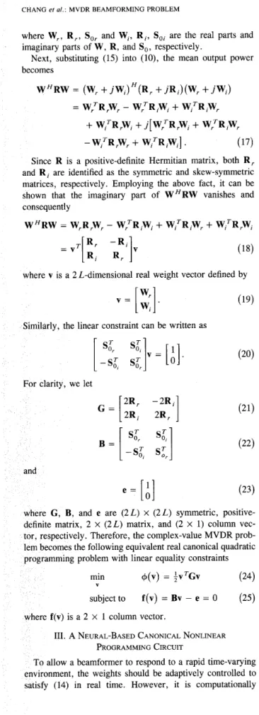
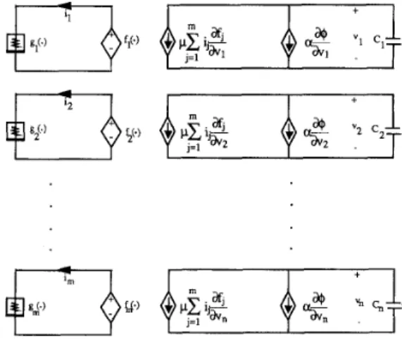
m
and n are two independent integers The canonical nonlinear programming ciFig. 1 consists of controlled current and voltage sources, nonlinear resistors, and linear capacitors. The voltages U, across the capacitors on the right-hand side of Fig. 1 repre- sent the values of the variables involved in the nonlinear programming. The currents
i,
through the voltage-controlled nonlinear resistors gJ(f,(v))
represent316 IEEE TRANSACTIONS ON ANTENNAS AND PROPAGATION, VOL. 40, NO. 3, MARCH 1992
site, resulting in the following expressions for P ( v ) :
5
I
g j ( f j ( v ) )I
,l m
- g3
(
f j ( v ))
, for square operator.2 j = 1
for absolute value j = 1
(30)
+-if+)
i
1-
j=lP ( v ) =
Moreover, the output of the jth constraint amplifier g j ( f j ( v ) ) can be defined as follows:
I I
Fig. 1. Canonical nonlinear programming circuit.
where v = [U,, u 2 ; * e , vJT. Note that the nonlinear func-
tions g j ( . ) are used to impose the constraints in the circuit realization. By reading directly from Fig. 1, the circuit equations for the network are given by
where
i j
= g j ( f j ( v ) ) , and both a and p are positive scaling factors.Next, we would like to show that the circuit equation of (28) converges to a minimum of the cost function 4(v) subject to a set of constraints. Before discussing this critical issue, several considerations involved in the constrained problem should be identified. The constraints in (27) define a subspace of the multidimensional parameter space called the feasibility region. Solving a constrained problems is, hence, the process of finding that point inside the corresponding feasibility region (including the boundary) where the value of the cost function 4(v) is the minimum one. To solve a constrained problem defined in (26) and (27), we convert it in an equivalent unconstrained problem. The way to do this is to define a pseudo-cost function E(v) as follows:
where $(v) is the original cost function, P ( v ) is referred to as the penalty function, and a and p are called the accelera- tion factor and the penalty multiplier, respectively.
Different penalty function alternatives can be used in prac- tice. Owing to the considerations in [8], [9], it can be concluded that for a function to qualify as a valid penalty function it must monotonically increase as the f j ( v ) deviates from the satisfaction of those constraints. In particular, either the absolute value or the square operator fulfills this requi-
for equality constraint (31) f j ( v > 9
=
1
U(
- f j ( v ) ) f j ( v ) , for inequality constraint whereU(.)
is the unit step function.It is interesting to note that the pseudo-cost function E(v) can be identified as energy function for the system of circuit equations (28) and the system is ensured to be completely stable. By complete stability, the system will not oscillate, but will converge to a stable equilibrium state. For simplic- itly of analysis, it is assumed the first-order time derivative of
E(v) exists and is continuous. In order to make the pseudo- cost function E(v) be differentiable, the square operator would be particularly considered in the penalty function. By using the fact that
i j
= g j ( f j ( v ) ) , the time derivative of E becomesI O . (32)
Since each c k is strictly positive and ( d v k / d t ) 2 2 O for all k , the time derivative of the pseudo-cost function E(v) is always less than zero. This implies that the circuit will force E(v) to be monotonically decreased except at the equilibrium points where the time derivative vanishes. Nevertheless, the equilibrium points may be either local minimum or inflection points of E(v). The second-order conditions, which are defined in terms of the Hessian matrix V2E(v) of second partial derivative of E(v), must be derived in order to determine the status of those equilibrium points. It is shown in [12] that the equilibrium point is a local minimum if the Hessian matrix of E(v) is positive-definite. Usually, the Hessian matrix V2E(v) is an n x n symmetric matrix de- fined by
a2E(v) VZE(V) = ~
[
a v i v j]
where vi is the ith component of v .By substituting (24) and (25) into (29), we have a
E ( v ) = -vTGv
+
~ ( B v - e)T(Bv-
e ) . (34) 2As a consequence, its Hassian matrix becomes
V2E(v) = a G
+
2 p B T B . (35) Since G and B T B are positive-definite and positive semidefinite, respectively, the Hassian matrix V2E(v) which is linear sum of G and BTB is positive definite. Therefore the equilibrium point is also the local minimum point. Further- more, the feasible region over which the constraints of (25) are satisfied can be shown to be a convex set. Since the Hassian matrix of (35) is positive definite throughout the feasible region, it is shown in [12] that any local minimum of E(v) is a global minimum over this feasible region. As a result, the circuit solution of the Hopfield-type network tends to a global minimum of the original cost function $(v) within the region over which the constraints are satisfied, when d E l d t = 0.IV
.
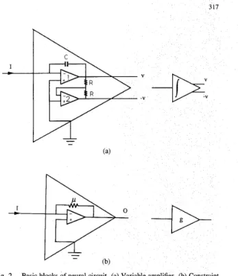
A NEURAL-BASED CIRCUIT IMPLEMENTATION FOR THE MVDR BEAMFORMING PROBLEMBasically, the circuit shown in Fig. 1 is used to solve a general nonlinear programming. In the case of MVDR-based constrained quadratic problem, a more compact neural-based circuit realization using the existing solid-state devices is possible. Usually, the circuit would include two particular modules. The first module is called the variable amplifier, which can perform the integral of a sum of (rn
+
1) input currents ( - a a 4 / a v k ) and (- piiafJ /auk) and then pro- duces the desired output variable v k . Fig. 2(a) shows the mplementation of the variable amplifier consisting of an integrator and a unity gain inverting amplifier. Op amp 1 Pro voltage v which is in proportion to the integral of the currentI.
The inverting amplifier including op amp 2 and resistorR
reproduces this voltage, but with opposite sign. The second module is called the constraint ich is used to perform the constraint satisfaction .). Since the MVDR problem has two equality constraints, the output of each gJ( a ) would be identical to itsinput. Therefore the circuit realization of gJ( e ) is particularly
simple and shown in Fig. 2(b). Without loss of generality, penalty multiplier p may be included in g j ( * ) . Thus, the uit yields the input-output relation: 0 =
-PI,
where prepresents the magnitude of the resistance, and 0 and I are an output voltage and an input current, respectively. If the input current I is equal to -fJ(v), then 0 = - p( -fJ(v)) =
hould be noted that the canonical nonlinear program- ming circuit model uses both current
i,
and voltage v k as variables. However, both iJ and uk are represented as "volt- ages" in the neural network implementation [lo]. By em- ploying the virtual short circuit property of the op amp [lo], these voltages would be converted to currents which are suitable for performing the weighted sum operation. Looking upon the circuit system dynamics of (28), the controlled pfJ(') = pgJ(fJ(')) =Fig. 2. Basic blocks of neural circuit. (a) Variable amplifier. (b) Constraint amplifier.
current sources
a
4
/a
vk and d f J/a
v k should be determined prior to the implementation. From (24) and (25), it follows thatand
where gk, and bJk are the ( k , i ) and ( j , k ) entries of G and B, respectively.
current
a4/avk
is a linear sum if the uk weighted by conductances gkl. In the case of linear constraints, the weights afJ(v)/avk are con- stants and so may be implemented directly as conductances. Combining (28), (36), and (37), one would obtain the state equations to the circuit implementation asEquation (36) shows that th
and
Note that the acceleration factor a is included in g k , and
then g;, is defined as (agk,).
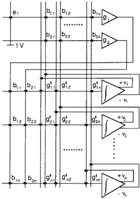
According to (38) and (39), a circuit realization is shown in Fig. 3. It should be noted that the elements of the e , G ,
318 IEEE TRANSACTIONS O N ANTENNAS AND PROPAGATION, VOL. 40, NO. 3, MARCH 1992
Fig. 3. Schematic diagram of neural circuit for MVDR-based beam forming problem.
and B matrices are realized directly as resistive connections
and that their associated matrix entries correspond to conduc- tance values. Considering the jth row of the upper constraint block, the input current Ij to the jth constraint amplifier is given by 2 L Ij = ej
+
bji( - U;) i = 1 L L =ej
-1
bjiui i = 1where e, = 1 and e2 = 0. Note that the resistor bjj is connected to the negative output terminal of the ith variable amplifier.
Thus, we would obtain the output voltage of the jth constraint amplifier as
p I j = p f j ( v ) . (41) i . = O = -
Since gLi and bjj are connected to the output terminal of the
ith variable amplifier and the output of the jth constraint amplifier respectively, the current Ik flowing into the kth variable amplifier is obtained by
2 L 2
I k =
1
g;jU;+
1
ijbjk. (42)i = 1 j = 1
By using the fact that Cduk / d t = - I k for the kth variable amplifier, it yields
As discussed in (40)-(43), it has been proven that the circuit schematic shown in Fig. 3 precisely implements the dynamic equation of (38) and (39) and then is applied to carrying out the optimal solution of the MVDR problem.
V. ILLUSTRATED EXAMPLES
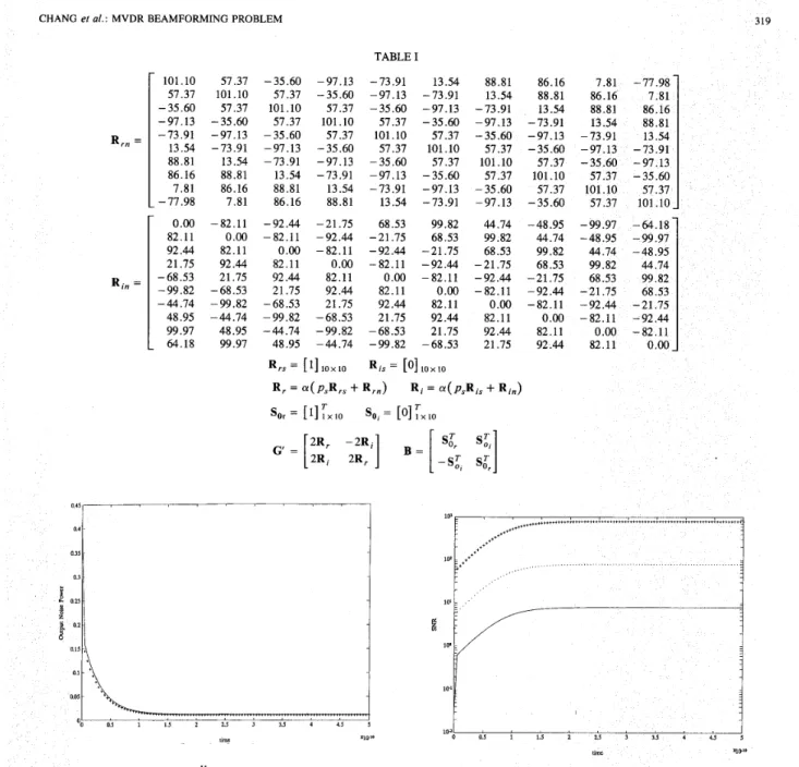
To verify the effectiveness of MVDR-based neural analog circuit implementation, a linear array of ten elements with half-wavelength spacing is considered in the following exam- ples. The variance of white noise present on each element, i.e, U," is assumed to be equal to 0.1. In addition, there are
two interference sources which fall in the main lobe and the first sidelobe of the conventional array pattern, respectively. The first interference makes an angle 72" (0, = 7 2 " ) with the line of the array and has the power which is taken to be 30 dB more than the white noise power. And, the second interference makes an angle of 98"(8, = 98") and has the power which is 10 dB more than the white noise power. Based on the above assumptions, it is concluded that the power levels for these two interferences would be identified as 100 and 1, that is, p , = 100 and p 2 = 1, respectively. The look direction of signal is assumed to be orthogonal to the array. Three signal powers varied from 0 to 20 dB above the white noise power are employed in our example.
The parameters gki and bjk involved in the proposed
circuit for this particular example could be obtained accord- ing to the value of each component in G and B. The
2 x 20(L = 10) matrix B includes two 10 x 1 vectors asso-
ciated with the look direction that are So, and So, shown in
Table I. Another 20 x 20 symmetric positive-definite matrix
G consists of both R , and R i which are 10 x 10 matrices in
terms of the signal power parameter p , and the acceleration
factor a . More details about the expression of G' are shown in Table I. In addition, the penalty multiplier p in each constraint amplifier and the acceleration factor a are taken to be 0.4 and respectively.
We have simulated the MVDR-based neural analog circuit described by (38) and (39) with the initial guess v(0) = 0,
using the simultaneous differential equation solver (DVERK in the IMSL). This routine solves a set of nonlinear differen- tial equations based on the fourth-order Runge-Kutta method. The capacitance C involved in each variable amplifier of the circuit is assumed to be 1 pF. Figs. 4 and 5 show the time evolutions of three output noise powers and the resulting output SNR's corresponding to their associated signal power levels 0.1, 1, and 10, respectively. It is worth observing that the converge time of each curve in Figs. 4 and 5 is almost independent of p s and equal to 0.1 ns. Since the converge
time is characterized by the time constant of system, one may use the dominant equivalent time constant 7 , which is defined in Appendix I to verify this particular time behavior. By using the G and B given in Table I, these dominant time
constants are found to be also independent of p , and equal to 5 x l o p 9 s. It has been shown that the converge time of each curve is bounded by the dominant time constant. In addition, while reaching the equilibrium state, those resulting solution weights do not satisfy both equality constraints exactly. Ap- pendix I1 shows that these two steady-state constraint viola-
Rrn = RI, =
:::I
101.10 57.37 -35.60 -97.13 -73.91 13.54 88.81 86.16 7.81 -77. 57.37 101.10 57.37 -35.60 -97.13 -73.91 13.54 88.81 86.16 7 . -35.60 57.37 101.10 57.37 -35.60 -97.13 -73.91 13.54 88.81 86. -97.13 -35.60 57.37 101.10 57.37 -35.60 -97.13 -73.91 13. -73.91 -97.13 -35.60 57.37 101.10 57.37 -35.60 -97.13 -73. 13.54 -73.91 -97.13 -35.60 57.37 101.10 57.37 -35.60 - 88.81 13.54 -73.91 -97.13 -35.60 57.37 101.10 57.37 - 86.16 88.81 13.54 -73.91 -97.13 -35.60 57.37 101.10 7.81 86.16 88.81 13.54 -73.91 -97.13 -35.60 57.37 1 --77.98 7.81 86.16 88.81 13.54 -73.91 -97.13 -35.60 57 0.00 -82.11 -92.44 -21.75 68.53 99.82 44.74 -48.95 - 82.11 0.00 -82.11 -92.44 -21.75 68.53 99.82 44.74 -48.95 -99.97 92.44 82.11 0.00 -82.11 -92.44 -21.75 68.53 99.82 44.74 -48.95 21.75 92.44 82.11 0.00 -82.11 -92.44 -21.75 68.53 -68.53 21.75 92.44 82.11 0.00 -82.11 -92.44 -21.75 6 -99.82 -68.53 21.75 92.44 82.11 0.00 -82.11 -92.44 - -44.74 -99.82 -68.53 21.75 92.44 82.11 0.00 -82.11 - 48.95 -44.74 -99.82 -68.53 21.75 92.44 82.11 0.00 -82.11 -92.44 99.97 48.95 -44.74 -99.82 -68.53 21.75 92.44 82.11 0.00 -82.11 - 64.18 99.97 48.95 -44.74 -99.82 -68.53 21.75 92.44 82.11 0.00-. Output noise power WHRNW versus the response time for a ement linear array with half-wavelength spacing. Two interferences are assumed: 8 , = 72", p , = 100, 0, = 98", p 2 = 1. U," = 0.1. The look direction angle is 90". The initial values of the weights are zero. '-':
p , = 0.1, '
. . .
'. . p , = 1, '+': p , = 10.tion errors could be estimated by e h , = 2 u p , / ( ~
+
up,) and eir, = 0. As a result, the penalty multiplier should be chosen large enough to make eik, sufficiently small. The final results are illustrated in the following table.Simulation Constraint Error
Theoretical Results Weighting Error Estimates
r SNR Value v(0) = 0 a! fi errl err2 eir, eir,
7.956 7.956 0.001 0.4 0.00056 0 0.0005 0 1 79.56 79.56 0.001 0.4 0.005 0 0.005 0 10 795.6 795.6 0.001 0.4 0.048 0 0.0488 0 It is worth simulating the case of large jammers by varying the INR's (interference-to-noise ratio) for both interfering
++,++,,,,r+++**t*+++*+++**.**+++++**+++++*******++**********~~*~.+***+**
16
+++*+++*+*~
trms
Fig. 5. Output signal-to-noise ratio versus the
ment linear array with half-wavelength spacing. Two interferences are assumed: 8 , = 72", pi = 100, O 2 = 98", p 2 = 1. U," = 0.1. The look direction angle is 90". The initial values of weights are zero. '-': p , = 0.1, ' . . . ' . . p , = 1, '+': p , = 10.
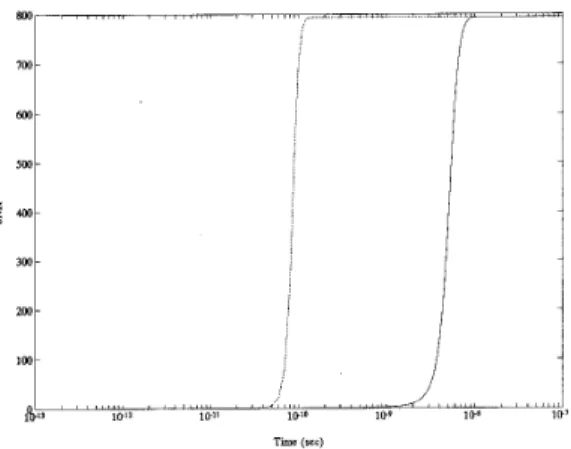
signals from 30-70
dB
simultane Fig. 6 shows that theresulting output SNR of each curve is almost independent of the same steady state level. Since the nto the variable amplifier is approximately proportional to the INR for the case of large jammers, it is expected that the converge time improves as INR increases. However, the acceleration factor is adjusted to smaller value in view of stability consideration and the dominant time constant in such case is about lop5 s. Another situation of particular interest is the performance evaluation of the beam- former under the influence of broad-band jammers. This is given by way of examples which demonstrate how the result- ing SNR varies as the element spacing changed from 0.35 A,,
320 IEEE TRANSACTIONS ON ANTENNAS AND PROPAGATION, VOL. 40, NO. 3, MARCH 1992
Tmc (rcc)
Fig. 6 . Output signal-to-noise ratio versus the response time for 10 element linear array with half-wavelength spacing. Two interferences are assumed: 8, = 72", 8 2 = 98". U,' = 0.1. The look direction angle is 90", p s = 10. The initial values of the weights are zero. '-': INR = 30 dB, '--': INR = 50 dB. '
...
': INR = 70 dB.to 0.75 X,, where
X,
is the wavelength and the signal source corresponds to the half-wavelength spacing. For comparison, all the parameter settings are taken to be the same as used in the previous case. One observes from Fig. 7 that the SNR starts to increase as the element spacing increases. It reaches its maximum level when the element spacing is equal to 0.68X,.
Beyond that the SNR level drops slightly. The reason is that the larger element spacing causes the grating lobes to appear in the array and thus degrades the overall output SNR. Finally, a comprehensive example is conducted to test the network performance for the case of closely spaced jammers. The phases of the interfering signals are assumed such that the angles of arrival for the two jammers are as close as O1 = 72" and O 2 = 74", respectively. The powers of both interferences are taken to be of the same level and equal to 100. The signal power, look direction angle and element spacing are suggested to be 10, 90" and 0 . 5 X, respectively. The resultant array output SNR is shown in Fig. 8 which reaches its maximum value of 950 rapidly. Fig. 9 comparesthe power patterns of the resultant adaptive array pattern with that of the conventional uniform array pattern. One observes clearly that two sharp nulls presented in the pattern corre- spond to the directions of arrival of the interferences. As a result, the interferences are suppressed and the output SNR
of the adaptive array reaches the optimal value. VI. CONCLUSION
In this paper, we have proposed a cost-effective analog circuit implementation for computing the MVDR beamform- ing problem based on Kennedy and Chua's cannonical neural network. Their novel neural-based optimizer is able to guar- antee the stability and robustness of the solution, the con- verge time can be characterized by the dominant time con- stant of the network. It turns out that the speed of reaching a steady-state solution depends essentially on the time constant, not on the algorithmic time complexity. Finally, a linear array of 10 elements with three signal levels is constructed accordingly to verify the performance of the proposed cir-
950!
558\5 0 4 0.45 0.5 0.55 0.6 065 0.7 0.!5
Narmalved element s p r i n g
Fig. 7 . Output signal-to-noise ratio versus the element spacing for a ten-element linear array. Two interferences are assumed: 8, = 72", p -
100, 8, = 98", p , = 100. U,' = 0.1. The look direction angle is ;O',
p s = IO. The initial values of the weights are zero.
l w o , , , , , ~ 1.5 2 25 3 I 3.5 4 4 5 5 "10" TmC
Fig. 8. Output signal-to-noise ratio versus the response time for a ten-ele- ment linear array with half-wavelength spacing. Two interferences are assumed: 8, = 72", p , = 100, 8, = 74", p z = 100. U,' = 0.1. The look direction angle is 90", p , = 10. The initial values of the weights are zero.
109, 0 20 40 M 80 1M 120 140 1M 8D.
De8
Fig. 9. The conventional uniform array pattern '--' and the resultant adaptive array pattern '-' for a 10-element linear array with half-wavelength spacing. Two interferences are assumed: 81 = 72", p1 = 100, 8, = 74",
p , = 100. U,' = 0.1. The look direction angle is 90", p s = 10. The initial values of the weights are zero.
cuit. It shows that the MVDR-based neural circuit is able to quickly attain its optimal performance in 0.1 ns when the dominant time constant is 5 x s and work satisfactorily under the stringent environment of strong jammers as well as closely spaced jammers.
APPENDIX I
THE DOMINANT TIME CONSTANT FOR AN MVDR-BASED NEURAL CIRCUIT
Substituting (38) into (39), one may obtain the system of first-order differential equations in matrix form and given by
d v 1
- = - -
[
( G+
pBTB)v+
pBTe] d t C= - M v + N e (44)
where M = ( G
+
pBTB)/C and N = -pBT/C.[ 1 11 showed that the solution of (44) can be expressed as a linear combination of modes tke-’rt where A, is the ith eigenvalue of M. It is known that the time behavior of system (44) would be dominated by the minimum eigenvalue
&,,,,(M) = min, (A,). Consequently, a dominant time con- stant for the MVDR-based neural circuit is defined by
(45) APPENDIX
II
ESTIMATION OF STEADY-STATE CONSTRAINT VIOLATION ERRORS
Let the steady-state constraint violation errors for both equality constraints defined in (25) be represented by err, and err2, respectively. While reaching the equilibrium state, these two constraints become
and 2 L
1
B,,u, = (1 - err,) k = 1 2 L1
B,,u, = err2. (47) k = 1Since the noise power pnoIse is assumed to be insignificant to the signal power, the objective function
4
is given byand the penalty function is calculated as
(49)
P = ;(err:
+
err;). Therefore, the energy function becomesE
I
steady state=
U 4
+
p P= + { 2 a p S ( 1 - err,)’
+
perrtBy the chain rule and the fact that dE/dt = 0 at the e rium state, the time derivative of E becomes
Equation (51) implies that both partial derivatives of E with respect to err, and err2 should vanish re
where eh-, and eir, are the es respectively. Then, we obtain
REFEREN
S. P. Applebaum, “Adaptive array,” ZEEE Trans. Antennas Prop-
agat., vol. AP-24, pp. 585-598, Sept. 1976.
B. Widrow and S. Steams, Adaptive Signal Processing. Engle- wood Cliffs, NJ: Prentice-Hall; 1985.
B. D. Van Veen and K. M. Buckley, “Beamforming: A versatile approach to spatial filtering,” ZEEE ASSP Mag., pp. 4-24, Apr. 1988.
L. C. Godara, “Error analysis of the tenna array proces- sors, ” IEEE Trans. Aerospace Elect
395-409, July 1986.
, vol. AES-22, pp. J. G. McWhirter and T. J. Shepherd, “Systolic array processor for
MVDR beamforming,” Proc. Inst. Elec. Eng., vol. 136, pt. F, no. 2, Apr. 1989.
W. M. Gentleman an Kung, “Matrix triangularisation by ea1 time signal processing IV, 1981, “Simple ‘neural’ optimization networks: An A/D converter, signal decision circuit, and a linear programming circuit,” ZEEE Trans. Circuit Syst., vol. CAS-33, pp. 533-541, May 1986.
L. 0. Chua and G. N. Li Feb. 1984.
322 IEEE TRANSACTIONS ON ANTENNAS AND PROPAGATION, VOL. 40, NO. 3, MARCH 1992 [9] M.P. Kennedy and L. 0. Chua, “Unifying the Tank and Hopfield
linear programming network and the canonical nonlinear program- ming circuit of Chua and Lin,” IEEE Trans. Circuit Syst., vol. CAS-34, pp. 210-214, Feb. 1987.
[lo] -, “Neural networks for nonlinear programming,” IEEE Trans. Circuit Syst., vol. 35, pp. 554-562, May 1988.
[ l l ] C. T. Chen, Linear System Theory and Design. New York: Holt, Rinehart and Winston, 1984.
[12] D. G. Luenberger, Linear and Nonlinear Programming, 2nd ed.
Reading, MA: Addison-Wesley, 1984.
Po-Rong Chang (M’87) received the B.S. degree in electrical engineering from National Tsing-Hua University, Taiwan, Republic of China, in 1980, the M.S. degree in telecommunication engineering from National Chiao-Tung University, Hsinchu, Taiwan, in 1982, and the Ph.D. degree from Pur- due University, West Lafayette, IN, in 1988.
From 1982 to 1984, he was a lecturer in the Chinese Air Force Telecommunication and Elec- tronics School for his two-year military service. From 1984 to 1985, he was an instructor of electri- cal engineering at National Taiwan Institute of Technology, Taipei, Taiwan. From 1989 to 1990, he was a project leader of SPARC chip design team at ERSO of Industrial Technology and Research Institute, Chu-Tung, Taiwan, Republic of China. Currently he is an Associate Professor of Communication Engineering at National Chiao-Tung University. His current interests include neural network, HDTV signal processing, and human visual and audio system.
Wen-Hao Yang was born in Chyi, Taiwan, Re- public of China, on June 12, 1964. He received the M.S. degree in communication englneenng from the National Chiao-Tung Umversity, Hsinchu, Tai- wan in 1988, where he is currently pursuing the Ph.D. degree.
From 1984 to 1986 he fulfilled h ~ s mditary duty by serving in the Chinese Air Force. Since 1988, he has been an assistant research engineer at the Telecommunication Laboratories, Ministry of Commumcations, Republic of China, where he works on satellite communication ground station establishment and mi- crowave filter design. His research interests are m adaptwe array, pattern synthesis, and rmcrowave circuits.
Kuan-Kin Chan (M’88) was born in China, in 1943. He received the B.S. degree in electrical engineering from Cheng Kung University in 1966, the M.S. degree in electronics from Chiao Tung University, Hsinchu, in 1969, and the Ph.D de- gree in electrophysics from Polytechnic Institute of Brooklyn, Brooklyn, NY, in 1976.
He is now a Professor in the Department of Communication Engineering, National Chiao Tung University, Taiwan, Republic of China. His cur- rent research interests are in the area of electro- magnetic scattering theory and applicahons.