A GENERAL PERFORMANCE ANALYSIS METHOD FOR UNIFORM MEMORY ARCHITECTURES

(1)

BIT 33 (1993), 536-560.

A G E N E R A L P E R F O R M A N C E A N A L Y S I S M E T H O D F O R U N I F O R M M E M O R Y A R C H I T E C T U R E S

JONG-JENG CHEN, CHIAU-SHIN WANG and CHING-ROUNG CHOU

Institue of Computer Science and A T & T Bell Laboratories, IH6U-213

Information Engineering, 2000, N. Naperville Rd.

National Chiao-Tun9 University, Naperville, 1L 60566, USA Hsin-Chu, Taiwan, R.O.C.

Abstract.

The performance of a multiprocessor system greatly depends on the bandwidth of its memory architecture. In this paper, uniform memory architectures with various interconnection networks including crossbar, multiple-buses and generalized shuffle networks are studied. We propose a general method based on the Markov chain model by assuming that the blocked memory requests will be redistributed to the memory modules in the next memory cycle. This assumption results in an analysis with lower complexity where the number of states is linearly proportional to the number of processors. Moreover, it can provide excellent estimation on the system power and memory bandwidth for all three types ofinterconnection networks as compared with the simulation results in which the blocked memory requests are resubmitted to the same memory module. Comparisons also show that our method is more general and precise than most existing analysis methods. The method is further extended to estimate the performance of multiprocessor system with caches. The approximation results are also shown to be remarkably good.

CR Categories: D.4.1., 1.2.8.

Keywords: multiprocessor system, interconnection networks, crossbar, multiple buses, generalized shuffle network, memory bandwidth, performance analysis, Markov chain.

1. Introduction.

With the advent of VLSI technologies, a great deal of attention has been paid to the design of multiprocessor systems to achieve higher computation power. How- ever, the performance ofa multiprocessor system greatly depends on the efficiency of its memory architecture. Memory architectures have been classified into two categories, N o n u n i f o r m - M e m o r y - A c c e s s ( N U M A ) a n d U n i f o r m - M e m o r y - A c c e s s

( U M A ) , As d e s c r i b e d in [ 1 ] , N U M A s y s t e m s a r e d i f f i c u l t t o p r o g r a m b e c a u s e t h e i r p e r f o r m a n c e is s e n s i t i v e t o t h e a l l o c a t i o n o f s h a r e d d a t a s t r u c t u r e s a n d m e m o r y m o d u l e s . I n U M A s y s t e m s , all s h a r e d m e m o r y is a c c e s s e d t h r o u g h a c o m m o n

(2)

A GENERAL PERFORMANCE ANALYSIS METHOD FOR . . . 537 interconnection network, so access time to any memory location is uniform across processors. This paper concentrates on the performance of UMA systems with various popular interconnection networks, such as crossbar, single bus, multiple buses, multistage interconnection networks and others.

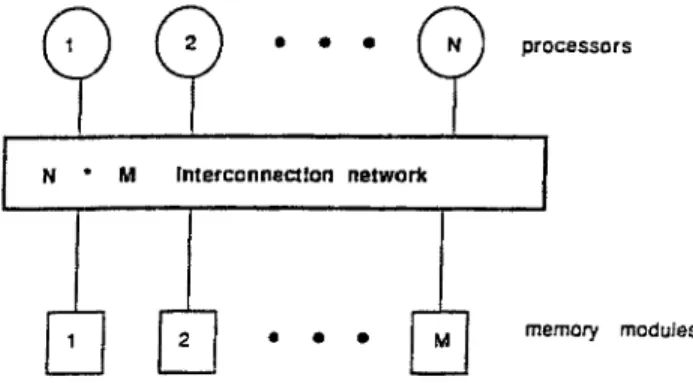
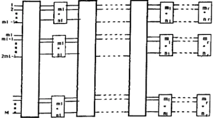
Early multiprocessor systems were implemented using crossbars, which allowed conflict-free connections between processors and resources. The needs of decreasing hardware cost and increasing number of processors drive the trend of using simpler interconnection structures, such as shuffle/exchange networks and multiple-buses. Figure I shows a general model of multiprocessor system with UMA architecture, where the big rectangle box can be any type of those interconnections.

Fig. 1. A simple multiprocessor system.

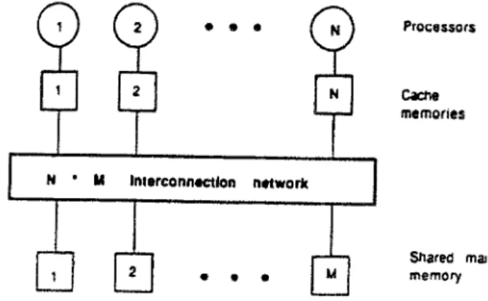
On the other hand, modern muttiprocessor systems often incorporate cache memory in each processor module in order to alleviate the data traffic through the interconnection networks. Such an architecture is conceptually depicted in Figure 2. The major drawback of the private cache is the data inconsistency problem, that is, the possibility of creating several copies of a single variable, where a copy is manipulated in a private memory independently of other copies, thus producing inconsistent values among those copies of the same variable. Such a problem can be solved through hardware or software interlocks and protocols. In the later analysis of UMA with cache memories, we shall assume an environment in which data consistency is not an essential problem and can be solved with implicit mechanisms embedded in the system.

In this paper, a general method which can be used for analyzing most of those interconnection networks in UMA architecture is presented. Crossbar, multiple buses and general shuffle networks (GSN) [2] are analyzed, where GSN is a very broad class of multistage interconnection networks. Some self-routing networks, such as Omega [3] and Delta [4] are its subclasses. It is shown that this method is not only more general but also very precise as compared with most existing analysis methods.

(3)

538 JONG-JENG CHEN, CHIAU-SHIN WANG AND CHING-ROUNG CHOU N " I e • Inlllrconnlcllon

Q)

E

network ~ ] Processors C4~:~e m e m o r i e s Shared nlaJn memory

Fig. 2. A multiprocessor system with private caches.

UMA architecture with crossbar interconnection. The first one is a Markov chain analysis proposed by Bhandrakar [53. It is very time consuming because of the enormous number of possible states. The second method was proposed by Strecker [6] for analyzing similar systems in which, if several processors happen to generate requests for accesssing the same memory, only one request will be accepted and all others will be missing. Although such an assumption may simplify the analysis, it will underestimate the memory bandwidth and thus the system power of a regular multiprocessor system. In [7], Yen et al. further modify the request rate to get an approximate memory bandwidth. However, this approach was applied to full crossbar interconnections only.

Since then, researches have been extended to the analysis of multiple-buses and multistage interconnection networks. Many researchers, such as Patel, Lang, Bhuyan, Das and Mudge have proposed quite a few interesting approaches [8-16]. However, some of them are not so general when analyzing all these three types of interconnection networks. Some of them may underestimate the bandwidth and the system power. We now present an alternative method which can be applied to estimate the performance o f U M A interconnection networks more generally and/or precisely than most existing approaches.

Our analysis method applied to the three types of UMA interconnection networks is presented in Section 2. The approximate analysis of the UMA system with private caches is presented in Section 3. Section 4 shows some analysis results and comparisons with a few well-known methods. A brief conclusion is given in Section 5.

2. Analysis of interconnection networks.

In this section, we focus on the analysis of the architecture shown in Figure 1, in which the interconnection networks can be crossbar, multiple buses or GSN. Before

(4)

A G E N E R A L P E R F O R M A N C E A N A L Y S I S M E T H O D F O R . . . 539

analyzing such systems, a few concepts and assumptions are required to clarify our presentation.

First, System Power is defined as the average number of busy processors in

a memory cycle. Bandwidth is the average number of busy memory modules in

a cycle. Waiting Time is the average time since a processor generates a request until it

gets the memory service. When we analyze the performance of such multiprocessor systems, these measures are used as fundamental indices. These three indices are closely related and given any one of them, the other two can be obtained. The less the waiting time is, the more the memory bandwidth can be utilized and thus the higher system power can be achieved. T h r o u g h o u t this paper, we will focus our interest on deriving the formulae for calculating these three performance indices for the systems consisting of various interconnection networks.

Our analysis is based on the technique of Markov Chain, which calculates the

probability of each possible state in the state space. In our study, we use the number

of busy processors in the system as the state of the system. The size of the state space is therefore linearly proportional to the size of the system. The following assumptions are made to simplify the state transitions in our analysis.

ASSUMPTION 1 : The system has N processors and M memory modules. It will be referred to as N x M system.

ASSUMPTION 2: All m e m o r y modules have equal constant cycle time and their operations are synchronous. All processors are identical and they all generate their requests at the beginning of a memory cycle.

A S S U M P T I O N 3: The processors and memories are connected by crossbar,

multiple buses or GSN, which allows every processor to have an access route to every m e m o r y module. The propagation delay and arbitration time in these interconnection networks are assumed to be ignorable. Alternatively, they may be considered as part of the memory cycle.

ASSUMPTION 4: F r o m each memory module, only one word can be accessed at a time. If two or more processors simultaneously make requests to the same memory module, only one of these requests can be served in that memory cycle. The other

processors will redistribute its request to the memory modules in the next memory

cycle. (The reason of this assumption will be explained later.)

A S S U M P T I O N 5: The conflict resolutions among processors in accessing the mem-

ory modules, buses and switches in crossbar and G S N are unbiased, i.e., there is no processor having the priority to get any particular path from itself to some memory module.

(5)

540 JONG-JENG CHEN, CHIAU-SHIN WANG AND CHING-ROUNG CHOU

and the request generated by a processor is independent of the request generated by another processor.

ASSUMPTION 7: The request generated in a cycle is independent of the request generated in the previous cycle.

ASSUMPTION 8: If the processor is not waiting for memory service, the process of

generating a request is a Bernoulli trial and we define p to be the request rate, i.e., the

probability that a processor generates a memory request.

Among the assumptions above, it seems that only Assumption 4 is a little bit

unrealistic because the requests blocked in a memory cycle are usually resubmitted

to the same memory module instead of being redistributed to some module in the

subsequent cycle. However, we shall show that this assumption may help to simplify the analysis but will cause little bias in the performance estimation. The simplifica- tion of the analysis will become clear in the derivation of the complete set of performance calculating formulae, and its unbiasedness will be illustrated by com- paring its analysis results with the simulation data of the real situation without this assumption in the later sections. The analysis results will also be compared with those results obtained by using other analytic methods.

2.1. Relations among performance indices.

A processor in the multiprocessor systems is assumed to be always in one of the two states, busy or waiting. It is either busy in doing certain useful work, or idle and waiting for the memory service. If we investigate the activities of a processor under our assumptions, it is easy to see that the relations among the three performance indices are independent of whether the interconnection networks is crossbar, multiple buses or GSN.

It

t t

t

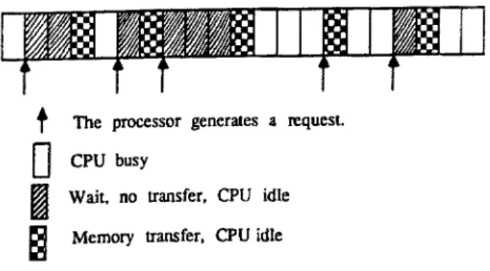
The processor generates a request. CPU busy

l ait, no transfer, CPU idle

Memory transfer, CPU idle

Fig. 3. The activity of a single processor.

t

(6)

A GENERAL PERFORMANCE ANALYSIS METHOD F O R . . . 541

Consider Figure 3, which shows a possible sequence of activities of a single processor. When a processor is not waiting for the memory service, it may generate a request with probability p and the probability that the processor does local computation is thus (1 -- p) in a cycle. If the processor does k computations, then

(1) p: (1 -- p) = x: k.

Thus the average number x of memory requests generated by the processor in k computations is

(2) x = kp/(1 - p).

Let m denote the average waiting time (number of waiting cycle) per memory request described above, then the processor utilization is

(3) U = k/(k + k(w + 1)p/(1 - p))

= 1/(1 + (w + 1)p/(1 - p)). The system power can thus be calculated as follows:

(4) P = N/(1 + (w + l)p/(l - p))

and the m e m o r y bandwidth is

(5) B W = N(kp/(1 - p))/(k + k(w + 1)p/(1 - p))

= P(p/(1 -- p)).

F r o m (3), (4), (5), if we can obtain any one of these performance indices, we actually know all the others.

2.2. General scheme.

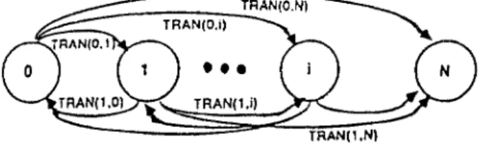
Imagine that we are now analyzing a multiprocessor system where all blocked requests will be redistributed in the next memory cycle. With this assumption the M a r k o v state can thus be represented by the number of requests in the beginning of a cycle. We define some notations as follows.

S~ is the state when there are i requests in the beginning of a cycle.

T R A N ( i , j ) is the probability that the state changes from Si to S~.

T H R U ( i , j ) is the probability that in the beginning of a cycle, there are i requests which pass through the interconnection network and j of them are accepted by memories.

GEN(i,j) is the probability that when there are i processors which are not waiting for the memory service in the beginning o f a cycle, j of them generate new requests.

F r o m Assumption 8, a processor will generate a request according to the Ber- noulli trial process. If there are i free processors, i.e., any of them can generate

(7)

5 4 2 JONG-JENG CHEN, CHIAU-SHIN WANG AND CHING-ROUNG CHOU

requests with probability p, then the process of generating requests is a binomial distribution with parameters i and p. Thus

(6) GEN(i,j) = pJ(1 -- p)(i-J) otherwise.

If we can get the value of THRUli,j) for all i and j, then

GEN(N,j) if i = 0

(7) TRAN(i,j) = ~i,=1 THRU(i,a) x

GEN(N - i + a,j - i + a) otherwise.

Thus we can establish the Markov state diagram as shown in Figure 4. This can be

T R A N ( O , N ~

TRAN(I i}

TRAN(1 .N)

Fig. 4. The discrete Markov state diagram for multiprocessor system.

easily solved by the Gauss elimination method or any other similar methods. Let

pr(i) be the probability of state Si. Then the system power is N

(8) P = ~ (N -i)pr(i).

i=o

Note that the number of states is exactly the number of processors. The solution of this Markov Chain is thus very easy to obtain and its complexity is only O(N3).

Now the major remaining problem is simply how to get the value of THRU(i,j). Its solution, of course, depends on the type of the interconnection networks. The following sections provide the solution of T H R U(i,j) for the crossbar, multiple buses and GSN, respectively.

2.3. Crossbar.

The crossbar architecture is shown in Figure 5. Because there is no conflict in the crossbar, the problem of solving T H R U(i,j) is equivalent to the occupancy problem with i balls and M urns where M is the number of memory modules.

(8)

A G E N E R A L P E R F O R M A N C E ANALYSIS M E T H O D FOR . . . 543 (9)

©

Q

O

switch

!

J"l ]

F

• I I •

O

O O 0

Fig. 5. T h e o r g a n i z a t i o n of c r o s s b a r i n t e r c o n n e c t i o n .

THRU(i,j) = I

0

ify<_i

and j_< M otherwise. 2.4.

Multiple buses.

p,oo~ssor ( )

B'I

j

memory y-

!

Fig. 6. An N x M x B m u l t i p l e b u s n e t w o r k .

The architecture of a multiple-bus system is shown in Figure 6, and we refer to it as an N x M x B system.

(9)

(t0)

THRU(i,j) =

544 JONG-JENG CHEN, CHIAU-SHIN W A N G AND C H I N G - R O U N G CHOU

The p r o b l e m of finding

THRU(i,j)

is similar to the occupancy problem with only

a small difference. If the n u m b e r of m e m o r y modules requested by the processors is greater than B, then only B requests can be accepted by memories. Thus

[~)ail°)(--lialj--a)(iJ~Ma)lifj<B~-~/(~'~-)i

= B Mx (~)~"=°xlx(a

\ M

J _

1 ) a " - - a i if j = B

0 otherwise.

2.5.

General shuffle network (GSN).

2 ~ m ! - 'Lo.. mt*l.~-- 2ml -,t--. M ~ m l i

Fig. 7. An M x N generalized shuffle network where M = ml x

mz x ... x mr

and

N ~ r t 1 X n 2 x . . . x n r .

A generalized shuffle network (GSN) [2] is a b r o a d class of networks. The M inputs connect to N outputs for any arbitrary values of M and N. Let M and N be

the products of r-terms such as M = ml x

mz x ... x mr

and N = nl x n2 x ... x hr.

An M x N G S N with M inputs and N outputs is an r-stage interconnection network as shown in Figure 7, consisting of a few crossbar switches of size rni x ni at the ith stage for all 1 < i ___ r.

This stage of G S N can be considered to consist of independent crossbars. If m o r e than one request at the input side of a crossbar attempts to reach the same link at the output side, then only one of these requests will be accepted, and the others are

rejected by the crossbar. Let

R(m, n, x, y)

be the probability that there are y requests

rejected

by a

single

crossbar given that there are x requests in the input side of the

m x n crossbar. By taking M = n, i = 1 a n d j = x - y in equation (9), it is easy to find that

(10)

A G E N E R A L P E R F O R M A N C E A N A L Y S I S M E T H O D F O R , . . 545

n ~ x - r - 1 x - - y x - - y - a

(11) R ( m , n , x , y ) = if x < _ m ^ y < _ n A y < _ x

0 otherwise.

Given h crossbar switches of size m x n, each having b input requests, let Q(h, m, n, b, d) be the probability that there are d rejected requests within the b x h requests to these crossbars. We can calculate this probability by solving recurrent equations as shown by the following lemma.

LEMMA 1. There exists a recurrent relation to calculate Q(h, m, n, b, d).

PROOF. By the notation of generating function and equation (I 1) which is the case of a single crossbar, Q(h, m, n, b, d) is the coefficient of x a in the following expression

(12) R(m, n, b, i)x i .

\ i = 0

We expand this to get the coefficient of x d, and the result is

b - 1

(13) Q ( h , m , n , b , d ) = ~ R(m,n,b, rl)Q(h - 1 , m , n , b , d - q)

r / = O

where the factor R(m, n, b, ~) in the right hand side of equation (13) can be considered as if the first crossbar rejected ~/requests and the factor Q(h - 1, m, n, b, d - rl) as if the other (h - 1) crossbars rejected (d - q) requests. It is trivial that Q(h, m, n, b, d) reduces immediately to R(m, n, b, d) when h = 1, i.e., it only has one crossbar. Thus

R ( m , n , b , d ) if h = 1

~'~Min(d,b-1) R i m n ~"

(14) Q ( h , m , n , b , d ) = ~,=Max(o,b-.) ~ . . . . q) ×

Q(h - 1, m , n , d , d - rl) if h > 1

0 otherwise. •

Let S(a, m, n, b, x, y) be the probability that, given that there are totally x requests in the input side of a crossbars with size m x n, there are y requests reaching output links, and each individual crossbar has at most b input requests.

THEOREM 1. There exists a recurrent relation to calculate S(a, m, n, b, x, y). PROOF. By the definition, the Product rule and the Sum rule, S(a, m, n, b, x, y) = ~ , ~pprob{[there are a crossbars having exactly b input requests] and [the crossbars will totally reject fl requests while any one of the ~ crossbars having exactly b input requests] and [given that there are totally (x - ~b) requests in the input sides of the remaining (a - ~) crossbars, any one of the (a - ~) crossbars has at

most (b - 1) input requests and (y - ab + t ) requests of them can reach the output links in the (a - c 0 crossbars]}.

(11)

546 JONG-JENG CHEN, CHIAU-SHIN W A N G AND C H I N G - R O U N G C H O U By lemma 1. S ( a , m , n , b , x , y ) = ~ \ ~ J \ b , ] \ x - ~ b )

<)

x Q ( c ~ , m , n , b - 1,fi) x S(a - e , m , n , b - 1 , x - ~ b , y - eb + fi).

Because there are ~ crossbars having b input requests and the (a - e) remaining crossbars have at most (b - t) input requests, therefore,

O < _ x - ~ b < _ ( b - ~ ) ( a - ~ ) and c~_>O. This implies that

Max(0, a + x - ab) <_ ~ <_ Lx/bJ.

F o r a single crossbar with b input requests, it would reject at most (b - 1) requests. Therefore for a crossbars each with b input requests, they totally reject at most e(b - 1) requests. Therefore

As a result, (15) S ( a , m , n , b , x , y ) = O _ < f l _ < ~ ( b - 1). 0 1 if x = y = 0 c z = M a x ( O ' a + x - a b ) / ~ f l = O O~ b x x S(a - •, m, n, b - t, x - ~b, y - c ~ b + fi) if ( b = 1 /x x C-y) or ( b = 1 /~ x = y / x x > a ) where a, m, n, x, y otherwise are all nonnegative integers.

Let tZab be the single-stage probability of having b requests surviving at the outputs of the ith stage of GSN, given a requests at the inputs of the ith stage. Let T i be the single-stage matrix of the ith stage such that T i = [r~b]-

Applying Theorem t, it is clear that

(16) tib = S(I, m, n, m, a, b)

where the ith stage of G S N consists of 1 crossbars with size of m x n.

(12)

A G E N E R A L P E R F O R M A N C E A N A L Y S I S M E T H O D F O R . . . 5 4 7

the ith stage, given no initial requests at the inputs of the first stage, and let G i be the

/-stage matrix such that G i _{= [g,o,,]}i , where i is found by applying (16) at each

gnoni

stage as follows.

1. The probability 1 g,o,~ of having nl outputs from the first stage, given that no

randomly generated inputs from the processors is given by (16),

2. Given nl inputs to the second stage, which are randomly distributed because we assume an unbiased conflict resolution policy at all stages, the probability of having n2 outputs at the second stage is given by

(17) _{g.o.~ = Prob}2 _[X2_{= n2 t X o = n o ]} N = ~ P r o b [ X 1 = n11Xo = n o ] P r o b [ X 2 = n 2 ] X l = nl] n l = 0 N 1 2 . 0 <_ no, n2 _< N = tnonltnln2 , h i = 0

where N is the number of the processors and the random variable X~, i # 0, is the number of the output links of the ith stage. The random variable Xo is the number of requests generated by the processors.

3. If n3 is the number of requests at the outputs of the third stage, we have similarly

N

(18) _gno.33 _E 2 3 . _{0 <_ no, n 3 <_ N .}

~--- gnon2 tn2n3,

//2=0

We generalize this process to get the input-output relation of an r-stage GSN as

N

( 1 9 ) r r - 1 -r

gnoNr ~ E 9,0 ... r,,~_ lnr 0 < no, nr-1, nr < N.

nr- 1

Clearly g,~o., is the r-stage probability; thus

(20) T H R U(no, nr) = gro,r.

Besides, let the r-stage matrix of these r-stage probabilities be denoted by G r, i.e., G~ = [g]b]- From (19), we have

(21) G r = (-I Ti. •

i = 1

The value of T I t R U(i,j) can thus be calculated for the crossbar, multiple-buses, and GSN according to equations (9), (10) and (20) respectively. As a result, the state transition probabilities and then the processor utilization, the system power as well as the memory bandwidth of the multiprocessor system can be easily obtained no matter which type of interconnection network is used.

(13)

548 JONG-JENG CHEN, CHIAU-SHIN WANG AND CttING-ROUNG CHOU

3. Approximate analysis of multiproeessor systems with private caches.

In a multiprocessor system with private caches as shown in Figure 2, the memory transfer time is no longer a single memory cycle. At each cycle, a cache may make a request to the main memory with probability m which is considered as proportional to the miss ratio. After a period of delay, a data transfer takes place. T h r o u g h o u t the whole cache miss period, the processor remains idle. A processor in our system is thus either busy doing computation or idle waiting for a cache miss service.

The crossbar, multiple bus and G S N interconnections will again be studied here. These networks will be assumed to operate in the circuit switching mode. Once a miss occurs in a cache, the cache miss handling hardware would request a block transfer from a particular main memory module and the network established a path between the cache and the main memory modules. This path is held until the memory access is completed. The path cannot be preempted by any other requests coming from other cache modules. In this description it is assumed that a block would reside in a single memory module. However, each m e m o r y module itself may be interleaved with others to increase the bandwidth. The advantage of using circuit switching and storing each individual block in one m e m o r y module is the reduction in block transfer time. In the three interconnection networks, there is an initial delay in establishing a path due to arbitration, decoding, and setting the appropriate switches. Once the path is established the data can be transferred at a higher rate.

In reality, there may be various types of requests in a multiprocessor system with private caches. Different types may have different request rate and transfer time. For example, in the simple write through protocol, there may be a read request for a block transfer and a store request for a single word transfer. In our analysis, we assume that the interconnection network assigns equal priority to all different requests.

T o analyze such systems, we adopted the approach used in [12] into our method. We apply our analysis with the modified request rate, which is derived from the original request rate of each type of the memory access and its transfer time, as seen by the interconnection network. The approximation is that t consecutive requests to a single memory module are decomposed into t separate requests which are randomly, independently and uniformly distributed over all modules. Although such a system condition is no longer equivalent to the original one, the offered traffic between the caches and the memory modules is not changed on the average.

Let us first examine a simple cache model in which each cache miss causes a period of waiting delay followed by t time units of data cache between a memory module and the cache. Consider Figure 8, which shows the situation of processor activities with respect to a few cache misses and waiting periods. Since in each processor cycle a cache miss may happen with probability m, there are on the average x faults for

(14)

A G E N E R A L P E R F O R M A N C E A N A L Y S I S M E T H O D F O R . . . 549

The processor generates a request CPU busy

Wait, no transfer, CPU idle Memory transfer, CPU idle

F i g . 8. T h e a c t i v i t y o f a s i n g l e p r o c e s s o r .

(22) x = kin/(1 -

m).

Let t be the block transfer time, then it has totally m k t / ( 1 - m ) time units spent in

block transfers within k units of useful computation.

Consider Figure 8 again, which shows the activity of a single processor. While a request is granted, the interconnection network maintains a path to a memory module for t time units. We can view this as t consecutive requests to the same module, each request requiring one time unit of service. Thus, from (22), it has

m k t / ( 1 - m) requests for unit service within k units of useful computation. Therefore, the request rate (for unit service) from a cache module as seen by the interconnection network is

(23) m' = [ m k t / ( 1 - rn)]/[k + m k t / ( 1 - m)] = mr~(1 - m + rot).

In the result we can apply the methods discussed above with such modified request rate, m', to each of the corresponding types of interconnection network.

F o r further elaboration, suppose that there exists a particular multiprocessor system which has i different types of requests. We define m, to be the request rate of the a-type request and t~ its transfer time.

Summarizing the activities of a single processor, we have

k : x l : x 2 : . . . : x i = (1 - ~ = 1 m ~ ) : r n l : m 2 " . . . : m l

where there are k time units of useful computation, and Xa is the average number of a-type requests. Thus

Xa = r e ° k / ( 1 - - 2 ~ = ~ m~) = y o k

where

i

yo = too~(1 - ~ = 1 m~).

(15)

• i

(24) m' = ~'~=1 y~t~k/(k + ~ = 1 y~t~k)

which is the request rate from a cache module as seen by the interconnection network. We can similarly apply the same method using such a modified request rate for analyzing the target interconnection networks connecting multiple processors/caches to memories.

4. Analysis results and comparisons.

4.1. Analysis and simulation results of interconnection networks without caches.

We now show some analysis results and the corresponding simulation results. The simulation was written in C and all memory requests were generated and distributed randomly. The simulation conditions and constraints follow the same assumptions as in our analytical model except that all rejected requests are resubmitted to the same memory module instead of redistribution at the next cycle. We show that Assumption 4 in our model would not impact the accuracy of the analysis results. The simulation was run for 400,000 time units. Each result is the mean of all those sample values taken every 20,000 time units for a total of 20 samples during the simulation run.

F r o m Tables 1, 2, 3, we can see that there is little difference between the computation and the simulation results. This is because a blocked request wilt eventually be submitted to a certain memory module. It makes little difference to consider it as a new request which is created and distributed to those memory modules. In a reasonable period of time the average traffic in the interconnection network and the workload of the memory modules thus stay the same as compared with the actual traffic where a blocked request will be resubmitted in the next cycle.

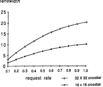
The m e m o r y bandwidths of crossbars, multiple buses and G S N are not listed because they can be obtained easily using Equation (5) based on Table 1, 2 and 3. F o r ease of comprehension, Figures 9 through 12 illustrate the trends of the analytical results ofbandwidths obtained with our method. The corresponding values of some curves can be found in Table 10 through t2.

4.2. Analysis and simulation results of interconnection networks with caches.

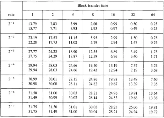
Tables 4, 5, 6 list several results obtained by using our approximate analysis of a multiprocessor system with private caches and compare them with the simulation results. The results are compared over a wide range of parameters. The varied parameters are: request rate m from 1/128 to 1/2, block transfer time t from 1 to 64 units.

(16)

A GENERAL PERFORMANCE ANALYSIS METHOD FOR . . . 551

T a b l e 1. The system power of N x M crossbar interconnection under various request rates, the number of processors is N and the number of memory modules is M.

16 x 16 32 x 32

rate analytical simulation analytical simulation

0.1 0.2 0.3 0.4 0.5 0.6 0.7 0.8 0.9 1.0 14.33 I2.54 10.67 8.80 6.98 5.28 3.73 2.33 1.10 0.00 14.34 12.56 10.65 8,80 7.01 5.29 3.70 2.33 1.10 0.00 28.65 25.15 2t.80 17.54 13.91 10.51 7.41 4.63 2.17 0.00 28.75 25.13 21.84 17.58 13.87 10.50 7.43 4.63 2.t7 0.00

T a b l e 2. The system power of N x M x B multiple bus interconnection, the number of processors is N, the number of memory modules is M and the number of buses is B.

rate 0.1 0.2 0.3 0.4 0.5 0.6 0.7 0.8 0.9 1.0 32 x 32 x 16 analytical 28.65 25.05 21.30 17.53 13.79 10.12 6.76 3.99 1.77 0.00 simulation 28.70 25.02 21.38 17.52 13.77 10.16 6.76 4.00 1.77 0.00 analytical 32 x 32 x 8 28.65 24,87 18.42 11.99 7.99 5.34 3.43 2.00 0.88 0.00 simulation 28.66 24.93 18.37 11.98 7.99 5.35 3.43 2.00 0.99 0.00

T a b l e 3. The system power of GSN interconnection.

rate 0.1 0.2 0.3 0.4 0.5 0.6 0.7 0.8 0.9 1.0 (4 x 4) x (4 x 4) analytical 14.29 12.36 10.37 8.30 6.40 4.71 3.25 2.00 0.91 0.00 t simulation 14.32 12.37 10.36 8.30 6.40 4.69 3.26 2.00 0.91 0,00 ( 8 x 4 ) x ( 4 x 8 ) analytical 28.38 23.96 19.i0 14.44 10.56 7.46 4.96 2.96 1.33 0.00 simulation 28.39 24.01 19.10 14.42 10.55 7.43 4.96 2.97 1.33 0.00

(17)

system power

3 0 ~ _ _ •

251"~4 ", - - 32x32 crossbar

/

~

-o-

32x32x16 multiple buses 2 0 \ -=- 32x32x8 multiple buses

+

\ \ o

lo

\

" ~ - -

0.1 0.2 0.3 0.4 0.5 0.6 0.7 0.8 0.9 1.0 request rate

Fig. 9. The system powers of crossbar and multiple-bus interconneetions.

bandwidth 25 2 0 o...-o "~ ' ° 1 5 _ ~ 1 5

0 ,,~,~i~,~.,~.,~..,...,---'--

! t i ~ l I i i | 0.1 0.2 0.3 0.4 0.5 0.6 0.7 0.8 0,9 1.0

request rate --,- 32 x 32 crossbar

-,,- 16 x 16 crossbar

Fig. 10. The memory bandwidth of crossbar interconnection networks.

In these three tables, the system powers obtained from our a p p r o x i m a t e method are a little bit higher than from the actual simulation. When the block transfer time is small, there is little difference between the c o m p u t a t i o n and the simulation results. The difference grows as the block transfer time increases. If we c o m p u t e the percentage of difference relative to the simulation result, the highest relative difference is 2 to 4 percent, which occurs when the block transfer time is 64. F o r most cases, the difference is less than 1 percent.

(18)

A G E N E R A L P E R F O R M A N C E ANALYSIS M E T H O D FOR . . . 553 b a n d w i d t h 16 _{j o t , ,} ~ - - _• _• _•

121

4 ./.

1o

. /

8 / / o - - - o ... 0 - - - - o - - - - 0 = ,,=, 6 4 2 0 0.1 0.2 0.3 0.4 0.5 0.6 0.7 0.8 0.9 1.0

request rate ._._ 32 x 32 x 1 6 muttiple buses 32 x 32 x 8 multiple buses Fig. 11. T h e m e m o r y b a n d w i d t h of m u l t i p l e - b u s i n t e r c o n n e c t i o n n e t w o r k s . b a n d w i d t h 1 4 12 10 8 6 4 2 0 0.1 0.2

o °51512151_-i

i / / i / " / ° 0.3 0,4 0.5 0.6 r e q u e s t r a t e q ! 4' I 0.7 0.8 0.9 1.0 - o - - {4 x 8) x (8 x 4) GSN - - - (4 x 4) x (4 x 4) GSN F'ig. 12. T h e m e m o r y b a n d w i d t h of G S N i n t e r c o n n e c t i o n n e t w o r k s .

As for the situation with multiple type of memory requests, we have applied the approximate method to the case with two types of request. One is word-request whose transfer time is one unit, and the other is block transfer. Tables 7, 8, and 9 compare the analytical and simulation results. The highest differences are 5 to 8 percent which occur when the transfer time is 16. For most cases, the differences are less than 2 percent.

(19)

554 JONG-JENG CHEN, CHIAU-SI-IIN WANG AND CIqlNG-ROUNG CHOU

T a b l e 4. The system power of crossbar interconnection with caches. The number of

processors is 32 and the number of memory modules 32. The upper part of each cell is the analytical result, and the lower part is the simulation result.

Block transfer time

rate 1 2 4 8 16 32 64 2-1 13.91 8.41 4.63 2.43 1.24 0.63 0.31 13.87 8.39 4.63 2.41 1.22 0.63 0.31 2 -2 23.20 17.64 1t.45 6.62 3.56 1.84 0.94 23.27 17.57 11.43 6.56 3.54 1.81 0.93 2 -3 27.77 24.23 18.90 12.75 7.54 4.11 2.14 27.80 24.29 18.89 12.63 7.36 3.95 2.07 2 -'~ 29.94 28.02 24.66 19.50 13.34 7.98 4.37 29.94 28.02 24.63 19.42 13.10 7.67 4.20 2 -s 30.98 30.00 28.15 24.86 19.78 13.63 8.20 30.98 29.99 28.12 24.84 19.68 13.27 7.92 2 -6 31.50 31.00 30.04 28.21 24.96 19.91 13.77 31.30 30.99 30.02 28.18 24.91 19.73 13.22 2 - 7 31.75 31.50 30.99 30.05 28.24 25.00 19.98 31.75 31.49 30.99 30.02 28.23 24.89 19.86

4.3. Comparison of analysis results between our method and others.

O u r m e t h o d is b o t h g e n e r a l a n d precise e n o u g h to a n a l y z e the p e r f o r m a n c e of a n y of c r o s s b a r s , m u l t i p l e buses a n d g e n e r a l i z e d shuffle n e t w o r k s . As s h o w n in the last section, the a n a l y s i s results are c o n s i d e r a b l y precise as c o m p a r e d w i t h the real s i m u l a t i o n in w h i c h the b l o c k e d m e m o r y requests are r e s u b m i t t e d to the s a m e m o d u l e i n s t e a d o f r e d i s t r i b u t i o n at the n e x t m e m o r y cycle. I n o r d e r to d e m o n s t r a t e the s u p e r i o r i t y of o u r m e t h o d , we p r e s e n t c o m p a r i s o n s w i t h o t h e r m e t h o d s a n d their a n a l y s i s results in this section.

T a b l e 10 lists the b a n d w i d t h s of the 32 x 32 c r o s s b a r u n d e r different r e q u e s t rates. I t is e a s y to see t h a t the d i s c a r d e d - r e q u e s t a p p r o a c h u s e d in [6] yields a result w h i c h u n d e r e s t i m a t e s the b a n d w i d t h b e c a u s e all b l o c k e d r e q u e s t s d u e to m e m o r y conflicts a r e d i s c a r d e d . T h e results f r o m b o t h Yen's m e t h o d [7] a n d o u r m e t h o d a r e v e r y close to the s i m u l a t i o n results. H o w e v e r , Yen's m e t h o d is a p p l i c a b l e o n l y to c r o s s b a r t y p e i n t e r c o n n e c t i o n s a n d is t h u s m o r e r e s t r i c t e d t h a n o u r m e t h o d .

T a b l e 11 lists the b a n d w i d t h s o f 32 x 32 x 16 a n d 32 x 32 x 8 m u l t i p l e buses u n d e r different r e q u e s t rates. D a s ' s m e t h o d [11] a l w a y s results in a l o w e r b a n d w i d t h e s t i m a t i o n . I t is a l s o b e c a u s e t h a t t h e b l o c k e d m e m o r y r e q u e s t s a r e a s s u m e d t o be d i s c a r d e d in D a s ' s m e t h o d . D a s ' s m e t h o d c a n be a p p l i e d o n l y to m u l t i p l e bus

(20)

A GENERAL PERFORMANCE ANALYSIS METHOD FOR . . . 555

Table 5. The system power of multiple bus interconnection with caches. The number of processors is 32, the number of memory modules 32 and the number of buses 16. The upper part of each cell is the analytical result, the lower is the simulation result.

Block transfer time

rate 1 2 4 8 16 32 64 2-1 13.79 7.83 3.99 2.00 0.99 0.50 0,25 13.77 7.71 3,93 1.93 0.97 0.49 0.25 2 z 23.19 17.53 11.15 5.95 2.99 1.50 0.75 22.28 17,73 11.02 5.79 2.94 1.47 0.74 2 -3 27.77 24,23 18.90 12.55 6.89 3.49 1,75 27.75 24.29 18.87 12.39 6.76 3.40 1.71 2 - 4 29.94 28.03 24.66 19.50 13.19 7.37 3.74 29.94 28,03 24,66 19.43 12.94 7.19 3.68 2 s 30.99 30.01 28.15 24.86 19.78 13.49 7.60 30.98 30.00 28.11 24.82 19.67 13.39 7.35 2 . 6 31.50 31.00 30.03 28.21 24.96 19.91 13,64 31.49 30,99 30,02 28.14 24.83 19.66 13.36 2 -~ 31.75 31.50 31.01 30.05 28,23 25.06 19,81 31.75 31.49 31.00 30,04 28.21 24.94 19.72

interconnection networks. Our method is therefore more precise and general than

Das's method. On the other hand, Mudge's method [t4] is based on a Semi-Markov

Interference model. It assumes that all rejected memory requests will be resubmitted to the same module in the next cycle. The analysis results of Mudge's method are very close to ours. Both are remarkably precise. The advantage of Mudge's method is that it can model variable connection time easily. However, its analysis applies only to multiple-bus systems and is therefore restricted, too.

Table 12lists the bandwidth of(4 x 4) x (4 x 4)GSN interconnection networks. Our method also results in higher bandwidth which is more precise than Patel's method [8]. The reason is that blocked memory requests are ignored in Patel's method. Patel's method cannot be applied to the analysis of multiple buses and is therefore also restricted.

From the comparisons above, it is obvious that our method is more general than most previous methods. It provides a fairly efficient analysis and can still yield precise results which are close to the real situation where the blocked memory requests are resubmitted to the same module in the next cycle.

(21)

556 T a b l e 6.

JONG-JENG CHEN, CHIAU-SHIN W A N G AND C H I N G - R O U N G CHOU

The system power of (4 x 8) x (8 x 4) GSN with caches. The upper part of each cell is the analytical result, the lower is the simulation result.

Block transfer time

rate 1 2 4 8 16 32 64 2 - t 10,56 5.74 2.98 1.50 0. 75 0.38 0.19 10.55 5.72 2.90 1,49 0,75 0.38 0.19 2 -2 21.55 14.44 8.28 4.37 2.23 1.13 0.57 22.58 14.39 8.22 4,36 2.22 1.12 0.57 2 -3 27.34 22.90 16.07 9.46 5.06 2.60 1.3t 27.38 23.00 16.04 9.44 5.06 2.60 1.30 2 - 4 29.84 27.65 23.46 16.80 10.02 5,40 2.78 29.87 27.67 23.42 i6.79 10.04 5.41 2.77 2 -5 30.96 29.91 27.79 23.71 17.15 10.29 5.57 30.96 29.91 27.77 23.70 17.12 10.30 5.57 2 -6 31.49 30.98 29.94 27.86 23.84 17.32 10.43 31.49 30.98 19.94 27.85 23.81 17.31 10.40 2 - 7 31,75 31,49 30,98 29.96 27.89 23.90 17.49 31.75 31,49 30.97 29,96 27,87 23,89 17,47

T a b l e 7. The system power of crossbar interconnection with caches and variable

requestin9 types. System ~ower m~ t~ mb tb 0.1 1 0.01 2 0.1 1 0.01 4 0.1 1 0.01 8 0.1 1 0.01 16 0.1 1 0.05 2 0.1 1 0.05 4 0.1 1 0.05 8 0.l 1 0.05 16 0.2 1 0.01 2 0.2 1 0.01 4 0.2 1 0.01 8 0.2 1 0.01 16 0.2 1 0.05 2 0.2 1 0.05 4 0.2 t 0.05 8 0.2 t 0.05 16 16 x 16 analysis simulation 14.00 I4.01 13.70 13.68 13.11 12.90 12.05 11.50 12.71 12.72 11.40 11.38 9.35 9.11 6.73 6.49 12.21 12,19 11.92 11.91 11.39 11.22 10.42 9.78 10.94 10.93 9.77 9,71 7.98 7.74 5.76 5.48 32 x 32 analysis simulation 27.99 28.00 27.38 27,35 26.21 26,14 24.08 23.24 25.40 25A0 22.78 22.6t 18.65 18.02 13.40 12.48 24.39 24.38 23.82 23.82 22.75 22.19 20,81 20_26 21.84 21.86 t9.45 19.36 t5.90 15.1t t 1.45 19,57

(22)

Table 8.

A GENERAL PERFORMANCE ANALYSIS METHOD FOR . . . 5 5 7

The system power of crossbar interconneetion with caches and variable requestin9 types. m 1 t~ m b t b 0.1 1 0.01 2 0.1 1 0.01 4 0.1 1 0.01 8 0.1 1 0.01 16 0.1 1 0.05 2 0.1 1 0.05 4 0.1 t 0.05 8 0.1 1 0.05 16 0.2 1 0.01 2 0.2 1 0.01 4 0.2 1 0.01 8 0.2 1 0.01 16 0.2 1 0,05 2 0.2 1 0.05 4 0.2 t 0.05 8 0.2 1 0.05 16 System power 16 x 16 32 x 32 analysis simulation 27.98 27.99 27.36 27.33 26.13 25.98 23.47 22.76 25.20 25.20 21.32 21.11 13.59 13.35 7.55 7,41 23.90 23.90 23.08 22.94 21.26 20.88 7.55 7.41 19.51 19.48 14.98 14.61 10.00 9.88 6.00 5.89 analysis simulation 27.99 28.00 27.38 27,35 26.21 26.14 24.08 23,24 25.40 25,40 22.78 22,67 18.64 18.06 13,25 12,44 24.39 24,37 23.82 23,81 22.75 22,54 13.25 12.44 21.84 21.83 19.39 19,32 15.86 15,59 11.15 10,72

Table 9. The system power of GSN interconnection with caches and variable

requesting types. rn 1 t~ na b t b 0.1 1 0.01 2 0.1 1 0.01 4 0.1 1 0.01 8 0.1 1 0,01 16 0.1 1 0.05 2 0.1 1 0,05 4 0.t 1 0.05 8 0.1 1 0.05 16 0.2 1 0.01 2 0.2 1 0.01 4 0.2 1 0.01 8 0.2 1 0.01 16 0.2 1 0.05 2 0.2 1 0.05 4 0.2 1 0.05 8 0.2 1 0.05 16 System power (8 x4) x ( 4 x 8) (4x4) x(4 x4) analysis simulation analysis simulation 27.60 27.62 26,87 26.71 25.43 25.22 22.71 21.86 24.40 24.39 21.02 20.97 i 4 . t 7 13.94 8.57 8.39 23.17 23.20 22.37 22.16 20.98 20.21 18.47 17,34 19.80 19.75 16.80 16.23 12.11 11.64 6.93 6.46 13.94 13.62 12.99" 11.84 12.56 11.13 8.89 5,82 12.01 11.70 10.96 9.01 10.63 9.35 6.72 4.28 13.94 13.62 12.87 11.21 12.54 11.01 8.46 5.53 12.12 11.69 10.67 8.57 10.72 9.22 6.54 4.14

(23)

558 T a b l e 10.

JONG-JENG CHEN, CHIAU-SHIN WANG AND CHING-ROUNG CHOU

The memory bandwidth of 32 x 32 crossbars. Comparison between our method, discard-request method and Yen's method.

t 32 x 32 crossbar

!

rate our method discard-request Yen's method

0.1 0.2 0.3 0.4 0.5 0.6 0.7 0.8 0.9 3.18 6.29 9.34 11.69 13.91 15.75 17.29 18.52 19.53 3.05 5.82 8.33 10.60 12.67 14.54 16.23 17.77 19.16 3.18 6.24 9.30 11.64 13.79 15.53 16.91 18.00 18.85

T a b l e 11. The memory bandwidth of 32 x 32 x 16 and 32 x 32 x 8 multiple buses. Comparison between our method. Das' s method and Mudge's method.

r a t e

32 x 32 x 16 multiple bus 32 x 32 x 8 multiple bus

our method Das's Mudge~s our method Das's Mudge's

0.1 3.17 0.2 6,26 0.3 9.t3 0.4 11.69 0.5 13.79 0,6 15.18 0.7 15.77 0.8 15,96 0.9 15.96 3.05 5.82 8.33 10.58 12.51 14.00 15.00 15.56 15.82 3.18 6.26 9.13 11.66 13.65 14.91 15.52 15.78 15.89 3.17 6.22 7.89 7.98 7,99 8.00 8.00 8.00 8.00 3.05 5.62 7.18 7.79 7.96 7.99 8.00 8.00 8.00 3.18 6.18 7.86 7.99 7.99 8.00 8.00 8.00 8.00

T a b l e 12. The memory bandwidth of(4 x 4) x (4 × 4 ) G S N . Comparison betweenour method and Patel' s method.

rate 0.1 0.2 0.3 0.4 0.5 0.6 0.7 0.8 0.9 ( 4 x 4 ) x ( 4 x 4 ) GSN our method 1.57 3.07 4.44 5.53 6.40 7.06 7.58 8.00 8.19 Patel's method 1.49 2.77 3.88 4.83 5.66 6.38 7.01 7.55 8.03

(24)

A GENERAL PERFORMANCE ANALYSIS METHOD FOR . . . 559

5. Conclusions,

We have presented a method to analyze the performance of interconnection networks in UMA architecture. The computation effort of this method is reason- ably low and the number of Markov states in the analysis is linearly proportional to the number of processors in the system. It provides a nice estimation of the performance of various interconnection networks for multiprocessor systems. Com- paring the analytical results with the results of simulation in a practical situation, the highest difference is less than 2 percent. Compared with a few well-known methods, our results are also shown to be more precise.

Another advantage of our method is its generality. The analytical model can be widely used in various interconnection networks. We have analyzed the crossbar, multiple buses and GSN interconnections. Since no restriction is made on the connection pattern between stages of GSN in our analytical model, this method can easily be extended to all multi-stage interconnection networks. The multi-stage interconnection networks may include Butterfly, Delta, Omega, Base-line, Reverse- exchange and others. For the UMA architecture with private caches, the difference between the analytical and the simulation results may increase as the length of the block transfer time increases. The largest difference is no more than 8 percent. For most cases, the differences are less than 2 percent. It shows that the accuracy of the approximate method is remarkably good.

However, our method does not apply to NUMA architecture. There is also some possible improvement which can be done in our model when analyzing the UMA architecture. A few assumptions could be modified to allow more practical situ- ations in a real multiprocessor system. For example, the processors and the memories may not be synchronized by a unified clock. They may run at different speeds. The interconnection delays may not be negligible, especially for a large multistage interconnection network. The path routing in the network and the accessing in the memory module may also be performed at a different pace. Any kind of these modifications on our original assumptions will result in a more complicated analysis. Whether they may have a significant impact on the analysis results will require further research efforts.

R E F E R E N C E S

1. M. Dubois and S. Thakkar, Cache architectures in tightly coupled multiprocessors, IEEE Computer, June 1990, pp. 9-11.

2. L. N. B h u y a n and D. P. Agrawal, Design and performance of generalized interconnection networks,

IEEE Transaction on Computer, voL C-32, Dec. 1983, pp. 1081-1090.

3. D. H. Lawire, Access and alignment of data in an array processor, IEEE Transaction on Computer, vol. C-24, Dec. 1975, pp. 1145-1155.

4. H . J . Siegel, Analysis techniquesJbr multiprocessors, IEEE Transaction on Computer, vol. C-29, Oct. 1980, pp. 771 780.

(25)

5. D. P. Bhandarkar, Analysis of memory interference in multiprocessor, IEEE Transaction on Com-

puter, vol. C-24, Sept. 1975, pp. 897-908.

6. W. D. Strecker, Analysis of the instruction execution rate in certain computer structures, Ph.D,

dissertation, Carnegie-Mellon University, 1970.

7. D. Yen, J. Patel and E. Davidson, Memory inteJference in synchronous multiprocessor systems, IEEE

Transaction on Computer, vol. C-31, Nov. 1982, pp. l l 16-1121.

8. J.H. ~ate~Pe~f~rmance~fpr~cess~r-mem~ryin~er~nnecti~n`~[brmultipr~cess~rs~EEETransa~ti~n

on Computer, vol. C-30, Oct. 1981, pp. 771-780.

9. T. Lang, M. Valero and I. Alegre, Bandwidth of crossbar and multiple-bus connection ofmultiproces- sots, IEEE Transaction on Computer, vol. C-31, Dec. 1982, pp. 1227-1234.

10. L. N. Bhuyan, An analysis of processor-memory interconnection networks, IEEE Transaction on

Computer, vol. C-34, Mar. 1985, pp. 279-283.

1 t. C.R. Das and L. N. Bhuyan, Bandwidth availability of multiple-bus muttiprocessors, IEEE Transac-

tion on Computer, vol. C-34, Oct. 1985, pp. 918-926.

12. J. H. Pate~ Analysis ~f multipr~ess~rs with private cache mem~ries~ IEEE Transacti~n ~n C~mputer,

vol. C-3L April 1982, pp. 296-304.

13. T.N. Mudge, J. P. Hayes, G. D. Buzzard and D. C. Winsor, Analysis of multiple-bus interconneetion networks, Proceedings of IEEE 1984 International Conference on Parallel Processing, Aug. 1984, pp.

228-232.

I4. T. N. Mudge and H. B. A~-Sad~un~ A Semi-Mark~v m~del f~r the perf~rmance ~f mu~tiple-bus systems`

IEEE Transaction on Computer, vol. C-34, Oct. 1985, pp. 934-942.

15. J. P. Sheu and W. T. Chen, PerJormance analysis ~" multiple bus interconnection networks with hierarchical requesting model, Proceeding of 8th IEEE Conference on Distributed Computing

Systems, June 1988, pp. 138-144.

16. Q. Yang and S. G. Zaky, Communication performance in multiple-bus system, IEEE Transaction on