This article was downloaded by: [National Chiao Tung University 國立交通大學] On: 28 April 2014, At: 05:01
Publisher: Taylor & Francis
Informa Ltd Registered in England and Wales Registered Number: 1072954 Registered office: Mortimer House, 37-41 Mortimer Street, London W1T 3JH, UK
International Journal of Systems Science
Publication details, including instructions for authors and subscription information: http://www.tandfonline.com/loi/tsys20
GA-based reinforcement learning for neural networks
CHIN-TENG LIN a , CHONG-PING JOU a & CHENG-JIANG LIN aa
Department of Electrical and Control Engineering , National Chiao-Tung University , Hsinchu, Taiwan, Republic of China
Published online: 16 May 2007.
To cite this article: CHIN-TENG LIN , CHONG-PING JOU & CHENG-JIANG LIN (1998) GA-based reinforcement learning for neural networks, International Journal of Systems Science, 29:3, 233-247, DOI: 10.1080/00207729808929517
To link to this article: http://dx.doi.org/10.1080/00207729808929517
PLEASE SCROLL DOWN FOR ARTICLE
Taylor & Francis makes every effort to ensure the accuracy of all the information (the “Content”) contained in the publications on our platform. However, Taylor & Francis, our agents, and our licensors make no representations or warranties whatsoever as to the accuracy, completeness, or suitability for any purpose of the Content. Any opinions and views expressed in this publication are the opinions and views of the authors, and are not the views of or endorsed by Taylor & Francis. The accuracy of the Content should not be relied upon and should be independently verified with primary sources of information. Taylor and Francis shall not be liable for any losses, actions, claims, proceedings, demands, costs, expenses, damages, and other liabilities whatsoever or howsoever caused arising directly or indirectly in connection with, in relation to or arising out of the use of the Content. This article may be used for research, teaching, and private study purposes. Any substantial or systematic reproduction, redistribution, reselling, loan, sub-licensing, systematic supply, or distribution in any
form to anyone is expressly forbidden. Terms & Conditions of access and use can be found at http:// www.tandfonline.com/page/terms-and-conditions
GA-based reinforcement learning for neural networks
CHIN-TENG LINt, CHONG-PING Jout and CHENG-JIANG LINt
A genetic reinforcement neural network (GRNN) is proposed to solve various rein-forcement learning problems. The proposed GRNN is constructed by integrating two feedforward multilayer networks. One neural network acts as an action network for determining the outputs (actions) of the GRNN, and the other as a critic network to help the learning of the action network. Using the temporal difference prediction method, the critic network can predict the external reinforcement signal and provide a more informative internal reinforcement signal to the action network. The action network uses the genetic algorithm (GA) to adapt itself according 10 the internal reinforcement signal. The key concept of the proposed GRNN learning scheme is to formulate the internal reinforcement signal as the fitness function for the GA. This learning scheme forms a novel hybridGA, which consists of the temporal difference and gradient descent methods for the critic network learning, and the GA for the action network learning. By using the internal reinforcement signal as the fitness function, the GA can evaluate the candidate solutions (chromosomes) regularly, even during the period without external reinforcement feedback from the environment. Hence, the GA can proceed to nell' generations regularly without waiting for the arrival of the external reinforcement signal. This can usually accelerate the GA learning because a reinforcement signal may only be available at a time long after a sequence of actions has occurred in the reinforcement learning problems. Computer simulations have been conducted to illustrate the performance and applicability of the proposed learning scheme.
I. Introduction
In general, the neural learning methods can be distin-guished into three classes: supervised learning, reinforce-ment learning and unsupervised learning. In supervised learning a teacher provides the desired objective at each
time step to the learning system. In reinforcement
learning the teacher's response is not as direct,
immediate or informative as that in supervised learning and serves more to evaluate the state of system. The presence of a teacher or a supervisor to provide the
correct response is not assumed in unsupervised
learning, which is called learning by observation.
Unsupervised learning does not require any feedback, but the disadvantage is that the learner cannot receive any external guidance and this is inefficient, especially for the applications in control and decision-making. If Received 5 July 1997. Revised 19 August 1997. Accepted 29 August 1997.
tDepartment of Electrical and Control Engineering, National Chiao-Tung University, Hsinchu, Taiwan, Republic of China.
supervised learning is used in control (e.g. when the input-output training data are available), it has been shown that it is more efficient than the reinforcement learning (Barto and Jordan 1987). However, many con-trol problems require selecting concon-trol actions whose consequences emerge over uncertain periods for which input-output training data are not readily available. In such a case, the reinforcement learning system can be used to learn the unknown desired outputs by providing the system with a suitable evaluation of its performance, so the reinforcement learning techniques are more appropriate than the supervised learning. Hence, in
this paper we are interested in the reinforcement
learning for neural networks.
For the reinforcement learning problems, Bartoet al.
(1983) used neuron-like adaptive elements to solve diffi-cult learning control problems with only reinforcement signal feedback. The idea of their architecture, called the actor-critic architecture, and their adaptive heuristic critic (AHC) algorithm were fully developed by Sutton (1984). The AHC algorithms that rely on both a learned 0020-7721/98 $12.00©1998 Taylor&Francis Ltd.
critic function and a learned action function. Adaptive critic algorithms arc designed for reinforcement learning with delayed rewards, The AHC algorithm uses the tem-pond difference method to train a critic network that Icarus to predict failurc. The prediction is then used to heuristically generate plausible target outputs at each time step, thereby allowing the use of backpropagation in a separate neural network that maps state variables to output actions. They also proposed the associative
reward-penalty(AR_I') algorithm for adaptive elements
culled A R-I' elements (Barto and Anandan 1985).
Several generalizations of AR_ P algorithm have been
proposed (Barto and Jordan 1987). Williams formulated
the reinforcement learning problem as a
gradient-following procedure (Williams 1987), and he identified a class of algorithms, called REINFORCE algorithms, that possess thc gradient ascent property. Anderson (1987) developed a numerical connectionist learning system by replacing thc neuron-like adaptive elements in thc actor-critic architecture with multilayer networks. With multilayer networks, the learning system can enhance its representation by Icarning new features that arc required by or that facilitate the search for the
task's solution. In this paper we shall develop a
rein-forccmcnt learning system also based on the actor-critic architecture, However, because the use of gradient descent (ascent) method in the above approaches usually
sutlers the local minima problem in the network
learning, we shall combine thc genetic algorithm (GA) with thc AHC algorithm into a novel hybrid GA for reinforcement learning to make use of the global opti-mization capability of GAs.
GAs arc general-purpose optimization algorithms
with a probabilistic component that provide a means to search poorly understood, irregular spaces. Holland (1975) developed GAs to simulate some of the processes observed in natural evolution. Evolution is a process
rluu operates on chromosomes (organic devices that
encode thc structure of living beings). Natural selection
links chromosomes with thc performance of their
decoded structure, The processes of natural selection cause those chromosomes that encode successful struc-turcs to reproduce more often than those that do not. Recombination processes create different chromosomes in children by combining material from the chromo-somes of thc two parents. Mutation may cause the chro-mosorncs of children to be different from those of their parents. GAs appropriately incorporate these features of natural evolution in computer algorithms to solve dif-fcrcnt problems in the way that nature has done through evolution. GAs require the problem of maximization (or minimization) to be stated in the form of a cost (fitness)
function. Ina GA a set of variables for a given problem
is encoded into a string (or other coding structure), analogous to a chromosome in nature. Each string
con-tains a possible solution to the problem. To determine how well a chromosome solves the problem, it is first broken down into the individual substrings which repre-sent each variable, and these values are then used to
evaluate the cost function, yielding a fitness value.
GAs select parents from a pool of strings (population) according to the basic criteria of survival of the fittest. It creates new strings by recombining parts of the selected parents in a random manner. In this manner, GAs are able to use historical information as a guide through the search space.
The GA is a parallel and global search technique. Because it simultaneously evaluates many points in the search space, it is more likely to converge toward the global solution. The GA applies operators inspired by the mechanics of natural selection to a population of binary strings encoding the parameter space at each generation, it explores different areas of the parameter space, and then directs the search to regions where there is a high probability of finding improved performance. By working with a population of solutions, the
algo-rithm can effectively seek many local minima and
thereby increases the likelihood of finding the global
minima. In this paper the GA is applied to find the
near-optimal weights of a neural network controller in the reinforcement learning environment.
Recent applications of GAs to neural network weight optimization produce results that are roughly
competi-tive with standard back propagation (Montana and
Davis 1989, Whitley et al. 1990). The application of
GAs to the evolution of neural network topologies has also produced interesting results (Harp et al. 1990, Schaffer 1990). There are domains, however, where GAs can make a unique contribution to neural network
learning. Inparticular, because GAs do not require or
use derivative information, the most appropriate appli-cations are problems where gradient information is una-vailable or costly to obtain. Reinforcement learning is one example of such a domain. Whitley et al. (1993) demonstrated how GAs can be used to train neural
net-works for reinforcement learning and neurocontrol
applications. They used the external reinforcemenl
signal from the environment directly as the fitness func-tion for the GA, and thus their system required the action network only. This structure is different from the actor-eritic architecture (Barto et al. 1983), which
consists of an action network and a critic network. In
our system we shall use a critic network to provide the action network with a more informative internal rein-forcement signal such that the GA can perform a more effective search on the weight space of the action net-work.
In this paper we propose a genetic reinforcement neural network (G RNN) to solve various reinforcement learning problems. The proposed learning system can
construct a neural network controller according to a reward-penalty (i.e. good-bad) signal, called the rein-forcement signal. It allows a long delay between an action and the resulting reinforcement feedback infor-mation. The proposed G RNN is constructed by
inte-grating two neural networks, each of which is a
feedforward multilayer network, and forms an actor-critic architecture. In the GRNN the network used as the action network can determine a proper action according to the current input vector (environment state). There is no 'teacher' to indicate the output errors of the action network for its learning in the rein-forcement learning problems. The other feedforward multilayer network (the critic network) can predict the external reinforcement signal and provide the action net-work with a more informative internal reinforcement signal, which is used as a fitness function for the GA-based learning of the action network.
Associated with the GRNN is a GA-based
reinforce-ment learning algorithm. Itis a hybrid GA, consisting of
the temporal difference method, the gradient descent method and the normal GA. The temporal difference method is used to determine the output errors of the
critic network for the multistep prediction of the
external reinforcement signal (Anderson 1987). With the knowledge of output errors, the gradient descent method (the back propagation algorithm) can be used to train the critic network to find proper weights. For the action network, the GA is used to find the weights for desired control performance. To optimize the con-nection weights of the action network, we encode these weights as a real-valued string (chromosome). In other words, each connection weight is viewed as a separate parameter and each real-valued string is simply the con-catenated weight parameters of the action network. Initially, the GA generates a population of real-valued strings randomly, each of which represents one set of connection weights for the action network. After a new real-valued string has been created, an interpreter uses this string to set the connection weights of the action network. The action network then runs in a feed-forward fashion to produce control actions acting on the environment. At the same time, the critic network pre-dicts the external reinforcement signal from the
con-trolled environment, and produces the internal
reinforcement signal to indicate the performance or fit-ness of the action network. With such evaluative infor-mation (fitness values) from the critic network, the GA can look for a better set of weights (a better string) for the action network.
The proposed GA-based reinforcement learning
scheme is different from the scheme proposed by
Whitley et al. (1993), especially in the definition of
fit-ness function. In this system there is no critic network, and the external reinforcement signal is used as the
fit-ness function of the GA directly in training the action network. Hence, an action network (defined by a string) can be evaluated only after the appearance of an external reinforcement signal, which is usually available only after very many actions have acted on the environ-ment in the reinforceenviron-ment learning problems. The major
feature of the proposed GA-based reinforcement
learning scheme is that we formulate the internal rein-forcement signal as the fitness function of the GA based on the actor-eritic architecture. In this way, the GA can evaluate the candidate solutions (the weights of the
action network) regularly even during the period
without external reinforcement feedback from the envir-onment. Hence, the GA can proceed to new generations regularly without waiting for the arrival of the external reinforcement signal. In other words, we can keep the time steps for evaluating each string (action network) fixed, because the critic network can give predicted reward/penalty information for a string without waiting for the final success or failure. This can usually accel-erate the GA learning, because an external reinforce-ment signal may be available only at a time long after a sequence of actions has occurred in the reinforcement learning problems. This is similar to the fact that we usually evaluate a person according to his/her potential or performance during a period, not after he/she has done something really good or bad.
This paper is organized as follows. Section 2 describes the basic of GAs and hybrid GAs. Section 3 describes the structure of the proposed GRNN. The corre-sponding GA based reinforcement learning algorithm is presented in section 4. In section 5 the cart-pole bal-ancing system is simulated to demonstrate the learning capability of the proposed GRNN. Performance com-parisons are also made in this section. Finally, conclu-sions are summarized in section 6.
2. Genetic algorithms
Genetic algorithms (GAs) were invented to mimic some of the processes observed in natural evolution. The underlying principles of GAs were first published by
Holland (1962). The mathematical framework was
developed in the 1960s and was presented by Holland (1975). GAs have been used primarily in two major areas: optimization and machine learning. In optimiza-tion applicaoptimiza-tions GAs have been used in many diverse fields such as function optimization, image processing, the travelling salesman problem, system identification and control. In machine learning GAs have been used to learn syntactically simple string IF-TH EN rules in an arbitrary environment. Excellent references on GAs and their implementations and applications can be found in
(Goldberg 1989, Davis 1991, Michalewicz and
Krawezyk 1992).
The encoding mechanisms and the fitness function form the links between the GA and the specific problem to be solved. The technique for encoding solutions may vary from problem to problem and from GA to .GA. Generally, encoding is carried out usmg bit stnngs. The coding that has been shown to be the optimal one is binary coding (Holland 1975). Intuitively, it is better
to have few possible options for many bits than to have
many options for few bits. A fitness function takes a chromosome as input and return a number or a list of numbers that is a measure of the chromosome's perfor-mance on the problem to be solved. Fitness functions play the same role in GAs as the environment plays in natural evolution. The interaction of an individual with its environment provides a measure of fitness. Similarly, the interaction of a chromosome with a fitness function provides a measure of fitness that the GA uses when carrying out reproduction.
The GA is a general-purpose stochastic optimization method for search problems. GAs differ from normal optimization and search procedures in .several ,:ays.
First, the algorithm works with a population ofstnng~,
searching many peaks in parallel. By employing genetic operators, it exchanges information between the peaks, hence lowering the possibility of ending at a local minimum and missing the global minimum. Second, it works with a coding of the parameters, not the para-meters themselves. Third, the algorithm only needs to evaluate the objective function to guide its search, and there is no requirement for derivatives or other auxiliary knowledge. The only available feedback from the system is the value of the performance measure (fitness) of the current population. Finally the transition rules are
prob-abilistic rather than deterministic. The randomized
search is guided by the fitness value of each string and how it compares to others. Using the operators on the chromosomes which are taken from the population, the algorithm efficiently explores parts of the search space where the probability of finding improved performance is high.
The basic element processed by a GA is the string formed by concatenating substrings, each of which is a In applying GAs for neural network learning, the
structures and parameters of neural networks are encoded as genes (or chromosomes), and GAs are then used to search for better solutions (optimal structures and parameters) for the neural networks. The funda-mental concepts of genetic operators and hybrid genetic algorithms will be discussed in the following sub-sections.
2.1. Basics of genetic algorithms
GAs are search algorithms based on the mechanics of
natural selection, genetics and evolution. It is widely
accepted that the evolution of living beings is a process that operates on chromosomes, organic devices that encode the structure of living beings. Natural selection is the link between chromosomes and the performance of their decoded structures. Processes of natural selec-tion cause those chromosomes that encode successful structures to reproduce more often than these that do not. In addition to reproduction, mutations may cause the chromosomes of biological children to be different from those of their biological parents, and recombina-tion processes may create quite different chromosomes in the children by combining material from the chromo-somes of two parents. These features of natural evolu-tion influenced the development of GAs.
Roughly speaking, GAs manipulate strings of binary digits, Is and as, called chromosomes which represent multiple points in the search space through proper encoding mechanism. Each bit in a string is called an allele. GAs carry out simulated evolution on popula-tions of such chromosomes. Like nature, GAs solve the problem of finding good chromosomes by manipu-lating the material in the chromosomes blindly without
any knowledge of the type of problem they are solving,
the only information they are given is an evaluation of
each chromosome that they produce. The evaluation IS
used to bias the selection of chromosomes so that those with the best evaluations tend to reproduce more often than those with bad evaluations. GAs, using simple manipulations of chromosome such as simple encodings and reproduction mechanisms, can display complicated behaviour and solve some extremely difficult problems without knowledge of the decoded world.
A high-level description of a GA is as follows (Davis 1991). Given a way or a method of encoding solutions to the problem on the chromosomes and a fitness (evalua-tion) function that returns a performance measurement of any chromosome in the context of the problem, a GA consists of the following steps.
Step I. Initialize a population of chromosomes.
Step 2. Evaluate each chromosome in the population.
Step 3.
Step 4.
Step 5.
Step 6.
Create new chromosomes by mating current chromosomes; apply mutation and recombina-tion on the parent chromosome's mate. Delete members of the population to make room for the new chromosomes.
Evaluate the new chromosomes and insert them into the population.
If the stopping criterion is satisfied, then stop and return the best chromosome; otherwise, go to Step 3.
binary coding of a parameter of the search space. Thus, each string represents a point in the seach space and hence a possible solution to the problem. Each string is decoded by an evaluator to obtain its objective func-tion value. This funcfunc-tion value, which should be max-imized or minmax-imized by the GA, is then converted to a fitness value which determines the probability of the individual undergoing genetic operators. The popula-tion then evolves from generapopula-tion to generapopula-tion through the application of the genetic operators. The total number of strings included in a population is kept unchanged through generations. A GA in its simplest form uses three operators: reproduction, crossover and
mutation (Goldberg 1989). Through reproduction,
strings with high fitnesses receive multiple copies in the
next generation, whereas strings with low fitnesses
receive fewer copies or even none at all. The crossover operator produces two offspring (new candidate solu-tions) by recombining the information from two parents in two steps. First, a given number of crossing sites are selected along the parent strings uniformly at random. second, two new strings are formed by exchanging alter-nate pairs of selection between the selected sites. Tn the simplest form, crossover with single crossing site refers to taking a string, splitting it into two parts at a ran-domly generated crossover point and recombining it with another string which has also been split at the same crossover point. This procedure serves to promote change in the best strings which could give them even higher fitnesses. Mutation is the random alteration of a bit in the string which assists in keeping diversity in the population.
2.2. Hybrid genetic algorithms
Traditional simple GAs, though robust, are generally not the most successful optimization algorithm on any particular domain. Hybridizing a GA with algorithms currently in use can produce an algorithm better than the GA and the current algorithms. Hence, for an opti-mization problem, when there exist algorithms, optimi-zation heuristics or domain knowledge that can aid in optimization, it may be advantageous to consider a hybrid GA. GAs may be crossed with various prob-lem-specific search techniques to form a hybrid that
exploits the global perspective of the GA (global
search) and the convergence of the problem-specific technique (local search).
There are numerous gradient techniques (e.g. the gra-dient descent method, the conjugate gragra-dient method) and gradient-less techniques (e.g. the golden search, the simplex method) available to find the local optimal in a calculus-friendly function (e.g. continuous function) (Luenberger 1976). Even without a calculus-friendly
function, there are well-developed heuristic search
schemes for many popular problems. For example, the greedy algorithms in combinatorial optimization are a form of local search (Lawler 1976). An intuitive concept of hybridizing GAs with these local search techniques is that the GA finds the hills and the local searcher goes and climbs them. Thus, in this approach, we simply allow the GA to run to substantial convergence and then we permit the local optimization procedure to take over, perhaps searching from the top 5% or 10% of points in the last generation.
Tn some situations hybridization entails using the
representation as well as optimization techniques
already in use in the domain, while tailoring the GA operators to the new representation. Moreover, hybrid-ization can entail adding domain-based optimhybrid-ization heuristics to the GA operator set. In these cases we can no longer apply the familiar GA operators directly and must create their analogue to account for new
repre-sentations and/or added optimization schemes. For
examples, Davis (1991) and Adler (1993) describe an approach to hybridizing a simple GA with the simulated annealing algorithm, and Tsinas and Dachwald (1994) and Petridis et al. (1992) describe an approach to hybri-dizing a simple GA with the back propagation
algo-rithm. A hybrid of both categories of learning
methods results in a more powerful, more robust and faster learning procedure. Tn this paper we develop a novel hybrid GA, called the GA-based reinforcement learning algorithm, to train the proposed GRNN to solve various reinforcement learning problems.
3. The structureofthe GRNN
Unlike the supervised learning problem in which the correct target output values are given for each input pattern to instruct the network learning, the reinforce-ment learning problem has only very simple evaluative or critic information available for learning, rather than instructive information. In the extreme case there is only a single bit of information to indicate whether the output is right or wrong. Fig. I shows how a network and its training environment interact in a reinforcement learning problem. The environment supplies a
time-varying input vector to the network, receives its
time-varying output/action vector and then provides a time-varying scalar reinforcement signal. In this paper
the reinforcement signal r(t) is two-valued,
r(t) E{-I,O}, such that r(t)
=
0 means a success andr(t) = -1 means a failure. We also assume that r(t) is
the reinforcement signal available at time step t and is
caused by the inputs and actions chosen at earlier time steps (i.e. at time steps t - I, t - 2, ... ). The goal of learning is to maximize a function of this reinforcement signal.
c.-
T.n h
v[l,
I+
I]
=Lbj[I]Xj[1
+ 11+
L
cdlJydl,
I+ I],
(3)
j=1 ;=1
y;[I,
I
+
1]
= g(t
aij[11.\j [I
+
11) , (I) J=IIand I
+
I are successive time steps, andaijis the weightfrom the jth input node to the ith hidden node. The
output node of the critic network receives inputs from
the nodes in the hidden layer (i.e. y;) and directly from
the nodes in the input layer (i.e ..\):
(2) I
g(s) = I+e-s'
internal reinforcement signal. The internal reinforce-ment signal from the critic network enables both the action network and the critic network to learn at each time step without waiting for the arrival of an external reinforcement signal, greatly accelerating the learning of both networks. The structures and functions of the critic network and the action network are described in the following subsections.
where
3.1. The critic network
The critic network constantly predicts the reinforce-ment associated with different input states, and thus equivalently evaluates the goodness of the control actions determined by the action network. The only information received by the critic network is the state of the environment in terms of state variables and whether or not a failure has occurred. The critic network is a standard two-layer feed forward network with sig-moids everywhere except in the output layer. The input to the critic network is the state of the plant, and the
output is an evaluation of the state, denoted by v.This
value is suitably discounted and combined with the external failure signal to produce the internal
reinforce-ment signal r(I).
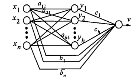
Figure 2 shows the structure of the critic network. It
includes h hidden nodes and n input nodes, including a
bias node (i.e. XI,X2,"" xn ) . In this network each
hidden node receives n inputs and has n weights, and
each output node receives n
+
h inputs and has n+
hweights. The output of the node in the hidden layer is given by
where v is the prediction of the external reinforcement
value, b, is the weight from the jth input node to output
node, and c, is the weight from the ith hidden node to
output node. In (I)and (3) double time dependencies are
used to avoid instabilities in updating weights
(Anderson 1987, Berenji and Khedkar 1992).
External
Reinforcement
. : Critic Network: V r
Signal
t
r
~emporalDifference Method: Internal
Reinforcement Stnte Signal
I
GeneticAlgorithm' X • Siring INeuralNetworkBuilderI
• Weights :Action Network:f
I
II
Plant IFigure 2. The structure of the critic network and the action network in the GRNN.
Figure I. The proposed genetic reinforcement neural network (GRNN).
To resolve reinforcement learning problems, a system called thc GRNN is proposed. As Fig. I shows, the GRNN consists of two neural networks; one acts as the action network and thc other as the critic network. Each network has exactly the same structure as that shown in Fig. 2. The G RNN is basically in the form of thc actor-critic architecture (Sutton 1984). As we want to solve the reinforcement learning problems in which the cxtcrnal reinforcement signal is available only after a long sequence of actions have been passed onto thc environment, we need a multistep critic net-work to predict the external reinforcement signal. In the GRNN, the critic network models the environment such that it can perform a multistep prediction of the cxternal reinforcement signal that will eventually be obtained from the environment for the current action chosen by the action network. With the multistep pre-diction, the critic network can provide a more informa-tivc internal reinforcement signal to the action network. The act ion net work can then determine a better action to impose onto the environment in the next time step according to the current environment state and the
The critic network evaluates the action recommended by the action network and represents the evaluated result as the internal reinforcement signal. The internal reinforcement signal is a function of the external failure signal and the change in state evaluation based on the
state of the system at time t
+
I:{
0, start state,
r(t
+
I)=
r[t+
I] - vlt, t], failure state,r[t
+
II
+
'"'fv[t, t+
I] - vlt, t]' otherwise, (4)where 0::::'"'f:::: I is the discount rate. In other words, the
change in the value ofI' plus the value of the external
reinforcement signal constitutes the heuristic or internal
reinforcement signal r(t) where the future values of v are
discounted more, the further they are from the current state of the system.
The learning algorithm for the critic network is com-posed of Sutton's AHC algorithm (Sutton 1984) for the output node and the backpropagation algorithm for the hidden nodes. The AH C algori thm is a temporal differ-ence prediction technique proposed by Sutton (1988). We shall go into the details of this learning algorithm in the next section.
3.2. The action network
The action network is to determine a proper action acting on the environment (plant) according to the cur-rent environment state. The structure of the action net-work is exactly the same as that of the critic netnet-work shown in Fig. 2. The only information received by the action network is the state of the environment in terms of state variables and the internal reinforcement signal from the critic network. As we want to use the GA to train the action network for control applications, we encode the weights of the action network as a real-valued string. More clearly, each connection weight is viewed as a separate parameter and each real-valued string is simply the concatenated weight parameters of an action network. Initially, the GA generates a popula-tion of real-valued strings randomly, each of which represents one set of connection weights for an action network. After a new real-valued string is created, an interpreter uses this string to set the connection weights of the action network. The action network then runs in a feed forward fashion to produce control actions acting on the environment according to (I) and (3). At the same time, the critic network constantly predicts the reinforcement associated with changing environment states under the control of the current action network. After a fixed time period, the internal reinforcement signal from the critic network will indicate the fitness of the current action network. This evaluation process
continues for each string (action network) in the popula-tion. When each string in the population has been eval-uated and given a fitness value, the GA can look for a better set of weights (better strings) and apply genetic operators on them to form a new population as the next generation. Better actions can thus be chosen by the action network in the next generation. After a fixed number of generations, or when the desired control per-formance is achieved, the whole evolution process stops, and the string with the largest fitness value in the last generation is selected and decoded into the final action network. The detailed learning scheme for the action network will be discussed in the next section.
4. GA-based reinforcement learning algorithm
Associated with the GRNN is a GA-based reinforce-ment learning algorithm to determine the proper weights of the GRNN. All the learning is performed on both the action network and the critic network simultaneously, and only conducted by a reinforcement signal feedback from the environment. The key concept of the GA-based reinforcement learning algorithm is to formulate the internal reinforcement signal from the critic network as the fitness function of the GA for the action network. This learning scheme is in fact a novel hybrid GA, which consists of the temporal difference and gradient descent methods for the critic network learning, and the GA for the action network learning. This algorithm possesses an advantage of all hybrid GAs: hybridizing a GA with algorithms currently in use can produce an algorithm better than the GA and the current algorithms. It will be observed that the proposed reinforcement learning
algorithm is superior to the normal reinforcement
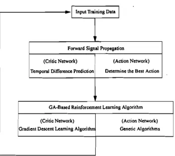
learning schemes without using GAs in the global opti-mization capability, and superior to the normal GAs without using temporal difference prediction technique in learning efficiency. The flowchart of the GA-based reinforcement learning algorithm is shown in Fig. 3. In the following subsections we first consider the reinforce-ment learning scheme for the critic network of the GRNN, and then introduce the GA-based reinforce-ment learning scheme for the action network of the GRNN.
4.1. Learning algorithm for the critic network
When both the reinforcement signal and input pat-terns from the environment depend arbitrarily on the past history of the action network outputs and the action network only receives a reinforcement signal after a long sequence of outputs, the credit assignment problem becomes severe. This temporal credit assign-ment problem occurs because we need to assign credit or blame to each step individually in long sequences
c.-which increases (decreases) its contribution to the total sum. The weights on the links connecting the nodes in the input layer directly to the nodes in the output layer are updated according to the following rule:
Note that the sign of a hidden node's output weight is used, rather than its value. The variation is based on Anderson's empirical study (Anderson 1987) that the algorithm is more robust if the sign of the weight is used, rather than its value.
where 7)
>
0 is the learning rate andr[1
+
II IS the internal reinforcement signal at time I+
I.Similarly, for the weights on the links between the hidden layer and the output layer, we have the following weight update rule:
cdl
+
I]
= C;[I]+
7)1'[1+
11.1';[1+
II. (6) The weight update rule for the hidden layer is based on a modified version of the error backpropagation algo-rithm (Rumelhart et al. 1986). As no direct error meas-urement is possible (i.e. knowledge of correct action is not available),r
plays the role of an error measure in the update of the output node weights; ifr
is positive, the weights are altered to increase the output v for positiveinput, and vice versa. Therefore, the equation for
updating the hidden weights is
aij[1
+
I]= aijlt]+
1/1'[1+
ILI';[I, 1](1 - Y;[I, l])sgn(c;[I].\j[I]. (7)4.2. Learning algorithm for the action network
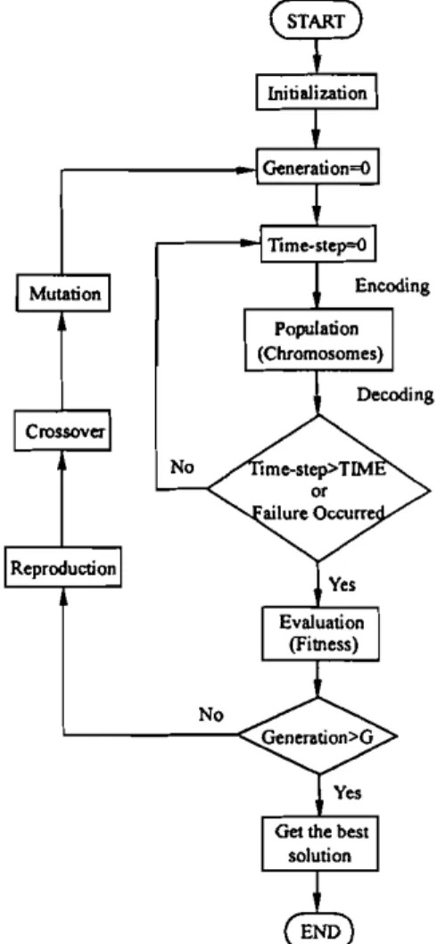
The GA is used to train the action network by using the internal reinforcement signal from the critic network as the fitness function. Fig. 4 shows the flowchart of the GA-based learning scheme for the action network. Initially, the GA randomly generates a population of real-valued strings, each of which represents one set of connection weights for the action network. Hence, each connection weight is viewed as a separate parameter and each real-valued string is simply the concatenated con-nection weight parameters for the action network. The real-value encoding scheme instead of the normal binary encoding scheme in GAs is used here, so recombination
can only occur between weights. As there are
(nX h
+
n+
17) links in the action network (see Fig. 2),each string used by the genetic search includes
(nx 17
+
n+
17) real values concatenated together. A small population is used in our learning scheme. The use of a small population reduces the exploration of the multiple (representationally dissimilar) solutions for the same network.After a new real-valued string has been created, an interpreter takes this real-valued string and uses it to
(5)
b;[1
+
I] = h;[I]+
7)1'[1+
I]x;it]'
I input Training DataI
Forward Signal Propagation
(Critic Network) (Action Network)
Temporal Difference Prediction Determine the Best Action
GA·BasedReinforcement Learning Algorithm
(CriticNetwork) (Action Network)
Gradient Descent Learning Algorithm Genetic Algorithms
Figure 3. Flowchart of the proposed GA-based reinforcement leurning algorithm for the G RN N.
leading up to cvcntuul successes or failures. Thus, to handle this class of reinforcement learning problems we need to solve the temporal credit assignment prob-Icm, along with solving the original structural credit assignment problem concerning attribution of network errors to different connections or weights. The solution to thc tcmporal credit assignment problem in GRNN is to usc a multistep critic network that predicts the rein-Iorccmcnt signal at each time step in the period without any external reinforcement signal from the environment. This can ensure that both the critic network and the action network can update their parameters during the period without any evaluative feedback from the envir-onmcnt. To train the multistep critic network, we use a technique based on the temporal difference method, which is often closely related to the dynamic program-ming techniques (Bartoet al. 1983, Sutton 1988, Werbos 1990). Unlike the single-step prediction and the super-vised learning methods which assign credit according to thc difference between the predicted and actual outputs, thc temporal difference methods assign credit according to thc difference between temporally successive predic-tions. Note that thc term multistep prediction used here means that the critic network can predict a value that will be available several time steps later, although it makes such a prediction at each time step to improve its prediction accuracy.
The goal of training the multistep critic network is to
minimize thc prediction error, i.e. to minimize the
internal reinforcement signal 1'(1). It is similar to a reward/punishment scheme for the weights updating in thc critic network. If positive (negative) interval rein-forccmcnt is observed, thc values of the weights are rewarded (punished) by being changed in the direction
(9)
Figure 4. Flowchart of the proposed hybrid GA for the action network.
set the connection weights in the action network. The action network then runs in a feedforward fashion to control the environment (plant) for a fixed time period (determined by the constant TIME in Fig. 4) or until a failure occurs. At the same time, the critic network
predicts the external reinforcement signal from the
controlled environment and provides an internal rein-forcement signal to indicate the fitness of the action
net-work. In this way, according to a defined fitness
function, a fitness value is assigned to each string in the population where high fitness values mean good
fit. The fitness function FIT can be any nonlinear,
non-differentiable, discontinuous, positive function,
because the GA only needs a fitness value assigned to each string. In this paper we use the internal reinforce-ment signal from the critic network to define the fitness function. Two fitness functions are defined and used in the G RNN. The first fitness function is defined by
I
FIT(I)
=
Ir(I)I' (8)which reflects the fact that small internal reinforcement values (i.e. small prediction errors of the critic network)
mean higher fitness of the action network. The second fitness function that we define is
I I
FlT(I)
=
Ir(I)1 x TIME'whereI is the current time step, I :::::: I :::::: TIME, and the
constant TIME is a fixed time period during which the performance of the action network is evaluated by the critic network. The added IITIME in (9) reflects the credibility or strength of the term 1/11'(1)1 in (8); if an action network receives a failure signal from the
envir-onment before the time limit (i.e. I :::::: TIM E), then the
action network that can keep the desired control goal longer before failure occurs will obtain higher fitness value. The above two fitness functions are different
from that defined by Whitleyet al. (1993). Their relative
measure of fitness takes the form of an accumulator that determines how long the experiment is still success. Hence, a string (action network) cannot be assigned a fitness value until an external reinforcement signal arrives to indicate the final success or failure of the current action network.
When each string in the population has been evalu-ated and given a fitness value, the GA then looks for a better set of weights (better strings) to form a new popu-lation as the next generation by using genetic operators introduced in section 2 (i.e. the reproduction, crossover and mutation operators). In basic GA operators, the crossover operation can be generalized to multipoint crossover in which the number of crossover point
(Nc ) is defined. With Nc set to I, generalized
over reduces to simple crossover. The multipoint
cross-over can solve one major problem of the simple
crossover; one-point crossover cannot combine certain combinations of features encoded on chromosomes. In the proposed GA-based reinforcement learning
algo-rithm, we choose Nc
=
2. For the mutation operator,because we use the real-value encoding scheme, we use a higher mutation probability in our algorithm. This is different from the traditional GAs that use the binary encoding scheme. The latter are largely driven by recom-bination, not mutation. The above learning process
con-tinues to new generations until the number of
generations meets a predetermined generation size (G in Fig. 4). After a fixed number of generations G, the whole evolution process stops, and the string with the largest fitness value in the last generation is selected and decoded into the final action network.
The major feature of the proposed hybrid GA learning scheme is that we formulate the internal rein-forcement signal as the fitness function for the GA based on the actor-eritic architecture (GRNN). In this way,
the GA can evaluate the candidate solutions (the
weights of the action network) regularly during the period without external reinforcement feedback from
system fails and receives a penalty signal of -I when
the pole falls past a certain angle(±12° was used) or the
cart runs into the bounds of its track (the distance is 2.4m from the centre to both bounds of the track).
The goal of this control problem is to train the
G RNN to determine a sequence of forces applied to the cart to balance the pole.
The model and the corresponding parameters of the cart-pole balancing system for our computer simula-tions are adopted from Anderson (1986, 1987) with the consideration of friction effects. The equations of motion that we used are
I • • I
, X ,
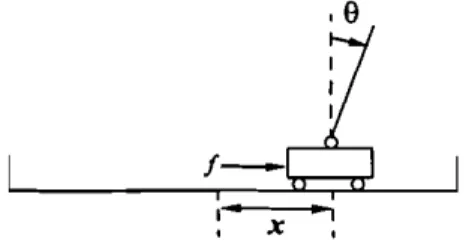
Figure 5. The cart-pole balancing system.
the environment. The GA can thus proceed to new gen-erations in fixed time steps (specified by the constant
TIM E in (9)) without waiting for the arrival of the
external reinforcement signal. In other words, we can e(1
+
I)= e(l)+
~e(I), (10). 2 I), (Ill
+
III )e(l)(Ill
+
IIlp)g sin e(l) - cos e(l)[f(l)+
IIlple(l) sin e(l) -JLcsgn(.Y(I))] - p p. . III /
O(I+I)=e(I)+~ p (II)
(4/3)(Ill
+
IIlp ) / - lIl/cos2 e(l)In the first set of simulations, we use the fitness
func-tion defined in (8), i.e. FlT(I) = I/lr(I)I, to train the
GRNN, where r(l) is the internal reinforcement signal
from the critic network. The used critic network and
X(I
+
I)= X(I)+
~.Y(I), (12)f(l)
+
IIlpl[e(I)2sine(l).( 1)- .() A -O(I)eose(I)]-I),csgn(.Y(I))
XI+ -XI
+u
( )
III
+
IIlp( 13)
whereg= 9.8 m/s2is the acceleration due to the gravity,
III
=
Ikg is the mass of the cart,IIlp=
0.1 kg is the massof the pole, /
=
0.5m
is the half-pole length,JLc=
0.0005is the coefficient of friction of the cart on the track,
JLp = 0.000002 is the coefficient of friction of the pole
on the cart, and ~ = 0.02 is the sampling interval.
The constraints on the variables are _12° ::;
e::;
12°,-2.4 m ::;x ::;2.4 m. In designing the controller, the
equations of motions of the cart-pole balancing
system are assumed to be unknown to the controller. A more challenging part of this problem is that the only available feedback is a failure signal that notifies the controller only when a failure occurs; that is, either
101
> 12° or [x]> 2.4 m. As no exact teachinginforma-tion is available, this is a typical reinforcement learning problem and the feedback failure signal serves as the reinforcement signal. As a reinforcement signal may only be available after a long sequence of time steps in this failure avoidance task, a multistep critic network with temporal difference prediction capability is used in the GRNN. The (external) reinforcement signal in this problem is defined as
keep the time steps TIME to evaluate each string
(action network) and the generation size Gfixed in our
learning algorithm (see the flowchart in Fig. 4), because the critic network can give predicted reward/penalty information to a string without waiting for the final success or failure. This can usually accelerate the GA learning because an external reinforcement signal may only be available at a time long after a sequence of
actions hasoccurred in the reinforcement learning
pro-blems. This is similar to the fact that we usually evaluate a person according to his/her potential or performance during a period, not after he/she has done something really good or bad.
S. Control of the cart-pole system
A general-purpose simulator for the GRNN model with
the multistep critic network has been written in the C
language and runs on an 80486-DX-based personal
computer. Using this simulator, one typical example, the cart-pole balancing system (Anderson 1987), is pre-scnted in this section to show the performance of the
proposed model.
The cart-pole balancing problem involves learning how to balance an upright pole as shown in Fig. 5. The bottom of the pole is hinged to a cart that travels along a finite-length track to its right or its left. Both the cart and pole can move only in the vertical plane; that is, each has only one degree of freedom. There are four
input state variables in this system:
e,
the angle of thepole from an upright position (deg);
e,
the angularvelo-city of the pole (dcgjs);x, the horizontal position of the
cart's centre (m); and .Y, the velocity of the cart (m/s).
Thc only control action isf, which is the amount of
force (N) applied to the cart to move it left or right.
This control action
f
is a discrete value,±
10 N. The{ - I r(l) = ' 0, ifle(I)I> 12°orlx(I)1 > 2.4m, otherwise. ( 14)
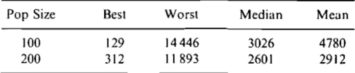
4780 2912 Mean 3026 2601 Median 14446 11893 Worst 129 312 Best 100 200 Pop Size
Table I. Performance indices of Whitley's system on the cart-pole balancing problem
work. Whitley et al. (1993) used a normal GA to update the action network according to their fitness function. Like the use of GRNN in the cart-pole problem, a bang-pole problem, a bang-bang control scheme is used in their system; the control output also
has only two possible values,
±
ION. The constraints onthe state variables are also _12° ::;0 ::;12°, -2.4m ::;
x ::; 2.4 m. The only available feedback is a failure signal that notifies the controller only when a failure occurs. The time steps from the beginning to the occur-rence of a failure signal indicate the fitness of a string (action network); a string is assigned a higher fitness value if it can balance the pole longer.
The simulation results of using Whitley's system on the cart-pole system for two different population sizes are shown in Table I. The first row of Table I shows the performance indexes when the population size is set as
POP
=
100. We observe that Whitley's system learnedto balance the pole at the 4780th generation on average. Whitley's system balanced the pole at the 129th genera-tion in the best case and at the 14446th generagenera-tion in the worst case. The median number of generations required to produce the first good action network (the network that is able to balance the pole for 100000 time steps) is 3026. The second row of Table I shows the performance
indexes when the population size is set as POP
=
200.The results show that Whitley's system learned to bal-ance the pole at the 2912th generation on average. In the best case, it took 312 generations to learn to balance the pole, and in the worst case it took II 893 generations to learn the task. The median number of generations required to produce the first good action network is
260I. From Table I we observe that the mean
genera-tion number needed by Whitley's system to obtain a good action network is more than 2500 generations. As compared to our system, the GRNN needs only
TIME
=
100 and G=
50 to learn a good actionnet-work.
From the point of view of CPU time, we compare the learning speed required by the GRNN to that by Whitley's system. A control strategy was deemed suc-cessful if it could balance a pole for 120000 time steps. When 120000 pole balance steps were completed, then the CPU times expended were measured and averaged over 50 simulations. The CPU times should be treated as 40
35
30
10 15 20 25
Time(second)
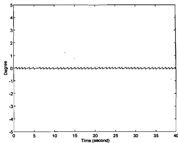
Figure 6. Angular deviation of the pole resulted by a trained GRNN withF1T(t)= I/lf(t)l. 5 4 3 2 $ "".
ir°
" 0 -1 -2 -3...
-5 0 5action network both have five input nodes, five hidden nodes and one output node. Hence, there are 35 weights in each network. A bias node fixed at 0.5 is used as the fifth input to the network; a weight from the bias node to a hidden node (or to the output node) in effect changes the threshold behaviour of that node. The learning parameters used to train the GRNN are the
learning rate 1]
=
0.1, the population sizes POP=
200,the time limit TIME = 100, and the generation sizes
G= 50. Initially, we set all the weights in the critic
net-work and action netnet-work to random values between -2.5 and 2.5. Mutation of a string is carried out by adding a random value to each substring (weight) in
the range
±
IO. The action network determines twoposs-ible actions
±
ION to act on the cart according to thesystem state. When the GA learning stops, we choose the best string in the population at the 50th generation and test it on the cart-pole system. Fig. 6 shows the pole position (angular deviation of the pole) when the cart-pole system was controlled by a well-trained GRNN
starting at the initial state: 0(0)
=
0, 1i(0)=
0,x(O)
=
0, .\'(0)=
O.The same cart-pole balancing control problem was also simulated by Whitley et al. (1993) using the pure GA approach. Whitley and his colleagues defined a fit-ness function different from ours. Their relative measure of fitness takes the form of an accumulator that deter-mines how long the pole stays up and how long the cart avoids the end of the track. Hence, a string (action net-work) cannot be assigned a fitness value before a failure
really occurs (i.e. either
101
>
12° or [x]>
2.4 m). As thefitness function was defined directly by the external rein-forcement signal, Whitley's system used the action net-work only. Their structure is different from our GRNN, which consists of an action network and a critic
c.-
T. Lin et al.Angulardeviationof the pole resulted by a trained
Whitley system. 3 2 4 5;r--~-~-~----'--~-~-~--' ·2
.,
-3 -5;L-_~-~--~-~-~-~~-~--o 5 10 15 20 25 30 35 40 Time (second)Figure 8. Angular deviation of the pole resulted by a trained
CRNN with1'1'1'(1)= I!Ii(I)Iafter a disturbance isgiven,
40 35 30 '" " ' " ..,, "'r' u "P' 15 20 25 Time(second) 10 Figure7. 244 5 4 3 2
~o
." 0 ·1 ·2 -3...
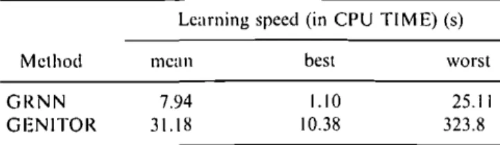
-5 0 5Table2. The learning speed in CI'U seconds ofC RNN and
GENITOR
Table3. Moriarty's results
Learning speed (in CPU TIM E(s)
Learning speed (in CPU'1'1ME) (s)
Method GRNN GENITOR mean 7.94 31.18 best 1.10 10.38 worst 25.11 323.8
Method mean best worst
one-layer AHC 130.6 17 3017
two-layer AHC 99.1 17 863
Q-Iearning 19.8 5 99
GENITOR 9,5 4 45
SANE 5.9 4 8
rough estimates because they arc sensitive to the imple-mentation details. However, the CPU time differences found arc large enough to indicate real differences in Iraining time on both methods. The results are shown
in Table 2.It is noted that the time needed to evaluate a
string in Whitley's system (called GENITOR in the table) is about three to four times as long as ours, as
our time steps arc bounded by the time limit TIMEand
by the arrival time of a failure signal, but the time steps for Whitley's system are bounded only by the arrival time of the failure signal. Hence, on average, the pro-posed hybrid GA is superior to the pure GA in learning speed in solving the reinforcement learning problems.' Fig. 7 shows the pole position (angular deviation of the pole) when the cart-pole system was controlled by a well-trained Whitley system starting at the initial state:
0(0)
=
0, 0(0)=
0, x(O)=
0, .\'(0)=
O. These angulardeviations arc slightly bigger than those produced by the trained GRNN.
For more complete performance comparisons, we consider several other learning schemes. Moriarty and Miikkulainen (1996) proposed a new reinforcement
learning method called SANE (symbiotic adaptive
ncuro-cvolution), which evolves a population of neurons through GAs to form a neural network capable of
per-forming a task. SANE achieves efficient learning
through symbiotic evolution, where each individual in the population represents only a partial solution to the problem; complete solutions are formed by combining several individuals. According to their results, SANE is faster, more efficient and more consistent than the
ear-lier AHC approaches (Bartoet al. 1983, Anderson 1987)
and Whitley's system (Whitleyet al. 1993) (as shown in
Table 3). From the table we found that the proposed GRNN is superior to the normal reinforcement learning schemes without using GAs for global optimization,
such as the single-layer AHC (Barto et al. 1983) and
two-layer AHC (Anderson 1987), and superior to the normal GAs without using temporal difference tech-nique (the GENITOR) in learning efficiency for rein-forcement learning problems.
Similarly to the simulations of Berenji and Khedkar
(1992), the adaptation capability of the proposed
GRNN was tested. To demonstrate the disturbance rejection capability of the trained GRNN, we applied
a disturbance
f
= 20 N to the cart at the IOth second.the curve of angular deviations in Fig. 8 indicates that the G RNN system brought the pole back to the centre
5,----~-~-~-~--~-~-~-, 5,----~-~-~-~-_~-~-~-, 4 4 3 3 2 1 ~ ~ .,.,~i~ ~
_.
''''';)''
.""..t .. "lO"
·r.", """ .""" -1 -2 -3 -3""
""
35 30 15 20 25 Time(second) 10 5.5,0
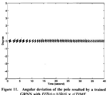
L--~-~--~---:'=----:;----::---:-::---:40 35 30 15 20 25 Time (second) 10 5 -5, 0 L--~-~---'::---:''---,':----::---:-::---:40Figure 9. Angular deviation of the pole resulted by a traiued GRNN withFlT(I)
=
1/1i"(t)1 when the half-length of the pole is reduced from 0.5 m to 0.25m,Figure II. Angular deviation of the pole resulted by a trained GRNN withFlT(I)= I/lr(I)1x IITIME.
5r--~-~--~-~--~-~-~---,
4
3
2
trained GRNN when the controlled system parameters are changed in the ways mentioned. The results show the good control and adaptation capabilities of the trained GRNN in the cart-pole balancing system.
In another set of simulations we use the second fitness function defined in (9), i.e.
I I FlT(t) =
Ir(I)1
x TIME'...
"
.,
~
o.}.-...
---'r"'"'...---w~
~ -1 -3 -2""
to train the GRNN. The goal of GA learning in the action network is to maximize this fitness function. The same learning parameters are used to train the GRNN in this case; the learning rate1)= 0.1, the popu-lation sizes PO P= 200, the time limit TIME
=
100, and the generation size G=
50. Fig. \1 shows the pole posi-tion when the cart-pole system was controlled by awell-trained GRNN system starting at the initial state:
0(0)= 0, e(O)= 0, x(O) = 0, .x-(O)= O. We also test the adaptation capability of the trained GRNN with the second fitness function. The curve of angular deviations in Fig. 12 shows that the G RNN brought the pole back to the centre position quickly after the disturbance
f
= 20 N was given at the 10th second. Figs 13 and 14show, respectively, the simulation results produced by the trained GRNN when we reduced the pole length
to I
=
0.25 m, and doubled the mass of the cart to/11
=
2 kg. The results also show the good control and adaptation capabilities of the trained G RNN with the second fitness function in (9) in the cart-pole balancing system. Comparing Fig. 13 to Fig. 9, we find that the GRNN trained by using the second fitness function in (9) is more robust than that by using the first fitness function in (8).In other simulations we tried to reduce the time limit TI M Eto 50 from 100 and kept the other learning
para-40
35 30 10 5 -5L--~-~=__-c'::_-__=---:~--=--___:=_______: o 15 20 25 Time(second)Figure 10. Angular deviation of the pole resulted by a trained GRNN withFlT(I)
=
I/lr(I)1when cart mass is doubled from I kg to2 kg.position quickly after the disturbance was given. In this
test, the G RNN required no further trials for
re-learning. We also changed the parameters of the cart-pole system to test the robustness of the GRNN. We
first reduced the pole length I from 0.5 m to 0.25 m.
Fig. 9 shows the simulation results produced by the
GRNN. It is observed that the trained GRNN can
still balance the pole without any re-Iearning. In another test, we doubled the mass of the cartmto 2 kg from I kg. Fig. 10 shows the simulation results produced by the GRNN. Again, the results show that the GRNN can keep the angular deviations within the range [_12°,
+
12°] without any re-learning. These robustness tests show that no further trials are required to re-Iearn a5'r--~-~--~-~-~----'--~--' < < 3 3 2
,
~0
~ .I.,.,~......
g ,'"
.~.,
2 1~ o,k<_'VI.-.."..,..."."""...."..."""...".'VIA~"""-v\.-'..."AV"""""''''''VY\'''''''''''''
III -1 ·2 -2..
·3..
Figure 12. Angular deviation of the pole resulted by a trained
GRNN with FlT(t)=I/li(t)1 x tlTlME after a
distur-bance is given, 35 30 10 5 -5L-_~_ _~ _ ~_ _~ _ ~_ _~ _ ~ ~ _ . J o 15 20 25 Time(18COl'Id)
Figure 14. Angular deviation of the pole resulted by a trained
GRNNwithF1T(t)= I/li(t)1x tl TlMl:when cart mass is doubled from I kg to 2 kg. 35 30 15 20 25 Time (second) 10 5
.,
-2 2 ReferencesADLER,D.,1993, Genetic algorithms and simulated annealing: a
mar-riage proposal. Proceedings of the IEEE International ConferenceOIl Neural Networks, Vol. II. San Francisco, CA, pp. 1104-1109. ANDERSON,C.W.,1986,Learning and problem solving with multilayer
connectionist systems. PhD thesis, University of Massachusetts; 1987, Strategy learning with multilayer connectionist repre-sentations. Proceedings of the Fourth International Workshop on Machine Learning, Irvine, CA, pp, 103-114.
BARTO, A.G., andANANDAN,P., 1985,Pattern-recognizing stochastic learning automata. IEEE Transactions on Systems. Man and Cyber-netics. 15.360-375.
the GA-based reinforcement learning algorithm was derived for the GRNN. This learning algorithm pos-sesses the advantage of other hybrid GAs; hybridizing a GA with algorithms currently in use can produce an algorithm better than the GA and the current algo-rithms. The proposed reinforcement learning algorithm
is superior to the normal reinforcement learning
schemes without using GAs in the global optimization capability, and superior to the normal GAs without using temporal difference technique in learning efficiency for reinforcement learning problems. Using the pro-posed connectionist structure and learning algorithm, a neural network controller that controls a plant and a neural network predictor that models the plant can be set up according to a simple reinforcement signal. The proposed GRNN makes the design of neural network controllers more practical for real-world applications, because it greatly lessens the quality and quantity requirements of the teaching signals, and reduces the long training time of a pure GA approach. Computer
simulations of the cart-pole balancing problem
satisfactorily verified the validity and performance of the proposed GRNN. <0 35 30 15 20 25 Time (second) 10 5 -5L...-_-,--~-~--~-~-~--~_.J o
Figure 13. Angular deviation of the pole resulted by a trained
GRNN with FIT(t)
=
I/li(t)1xtlTlME when thehalf-length of the pole is reduced from 0.5 m to 0.25 m.
5r---'---'--~~-'---'---'--~--'
..
<
3
6. Conclusion
This paper describes a genetic reinforcement neural net-work (GRNN) to solve various reinforcement learning problems, By combining the temporal difference tech-niquc, thc gradient descent method and genetic algo-rithms (GAs), a novel hybrid genetic algorithm called meters unchanged. After computer simulations, the results also show the good control and adaptation cap-abilities of the trained G RNN in the cart-pole balancing system. However, on average, the learned best action network is not so good in angular deviation as those
in the above simulations using TIME
=
100.BARTO, A. G .. and JORDAN, M. I., 1987, Gradient following without backpropagution in layered network. Proceedings of the lnterna-tional Joint Conference on Neural Networks, San Diego, CA, Vol.
II, pp. 629-636.
BARTO, A. G .. SUTTON, R. S., and ANDERSON,C.W., 1983, Neuron-like adaptive elements that can solve difficult learning control
pro-blem.IEEE Transactions on Svstcrns. Alan ond Cybemetics,
13,834-847.
BERENJI, H. R., and KHEDKAR,p ..1992, Learning and tuning fuzzy logic controllers through reinforcements. IEEE Transactions on Neural Networks, 3, 724-740.
DAVIS,L., 1991. Handbook: of Genetic Algorithms (New York: Van
Nostrand Reinhold).
GOLDBERG. D. E..1989.Genetic Algorithms in Search, Optimization ami Machine Leurning (Reading, MA: Addison-Wesley).
HARP, S., SAMAD, T., and GUHA, A., 1990, Designing application-specific neural networks using the genetic algorithm. Neural In/ormation Processing Systems. Vol. 2 (San Mateo, CA: Morgan
Kaufman),
HOLLAND,J. H., 1962, outline for a logical theory of adaptive systems.
Journal of the Association for Computing Machinery, 3, 297-314; 1975. Adaptation in Natural and Artificial System (Ann Arbor, MI:
University of Michigan).
LAWLER, E. L., 1976. Combinatorial Optimization: Networks and
Matroids (New York: Holt, Rinehart and Winston).
LUENBERGER,D. G.,1976,Linear lind Nonlinear Programming
(Read-ing, MA: Addison-Wesley).
MICHALEWICZ, Z" and KRAWEZYK, J. B., 1992, A modified genetic algorithm for optimal control problems. Computers and Mathema-tical Applications. 23, 83-94.
MONTANA, D., and DAVIS,L.,1989, Training feedforward neural net-works using genetic algorithms. Proceedings of the International Joint Conference on Artificial Intelligence. pp. 762-767.
MORIARTY, D. E., and MIIKKULAINEN, R., 1996, Efficient reinforce-ment learning through symbiotic evolution. Machine Learning. 22,
11-32.
PETRIDIS, V., KAZARLlS, S., PAPAIKONOMOU, A., and FILELlS, A., 1992, A hybrid genetic algorithm for training neural networks. Arti-ficial Neural Networks 2. edited by I. Aleksander and J. Taylor,
(North-Holland), pp. 953-956.
RUMELHART, D., HINTO, G., and WILLIAMS, R. J.. 1986, Learning internal representation by error propagation. Parallel Distributed Processing, edited by Rumelhart, D., and McClelland (Cambridge,
MA: MIT Press), pp. 318-362.
SCHAFFER, J. D., CARUANA, R. A., and ESHELMAN,L.J" 1990, Using genetic search to exploit the emergent behavior of neural networks.
Physico D, 42, 244-248.
SUTTON, R. S., 1984, Temporal credit assignment in reinforcement learning. PhD thesis, University of Massachusetts, Amherst, MA, USA; 1988, Learning to predict by the methods of temporal
differ-ence.Machine Learning, 3, 9-44.
TSINAS,L. and DACHWALD, B., 1994, A combined neural and genetic learning algorithm. Proceedings of the IEEE International Confer-ence on Neural Networks,vol.I, pp. 770-774.
WERBOS, P.J., 1990. A menu of design for reinforcement learning over time.Neural Networks for Control, edited by W. T. Miller, III, R. S.
Sutton, and P. J. Werbos (Cambridge: MIT Press), Chapter 3. WHITLEY, D., DOMtNIC, S., DAs, R., and ANDERSON,C.W" 1993,
Genetic reinforcement learning for neurocontrol problems.Machine Learning, 13, 259-284.
WHITLEY, D" STARKWEATHER, T" and BOGART, c., 1990, Genetic algorithm and neural networks: optimizing connections and connec-tivity. Parallel Computing, 14,347-361.
WILLIAMS, R, 1., 1987, A class of gradient-estimating algorithms for reinforcement learning in neural networks. Proceedings of the International Joint Conference on Neural Networks, San Diego.
CA, Vol. II, pp. 601-608.