IEEE 802.16e OFDMA實體層測距技術與數位訊號處理器實現之探討

國 立 交 通 大 學

電

子工程學系

電

子研究所碩士班

碩

士

論

文

IEEE 802.16e OFDMA實體層測距

技術與數位訊號處理器實現之探討

Study in Ranging Techniques and Associated Digital Signal

Processor Implementation for IEEE 802.16e OFDMA PHY

研 究 生：蔡昀澤

指導教授：林大衛 博士

IEEE 802.16e OFDMA 實體層測距

技術與數位訊號處理器實現之探討

Study in Ranging Techniques and Associated Digital Signal

Processor Implementation for IEEE 802.16e OFDMA PHY

研究生:蔡昀澤

Student:

Yun-Tze

Tsai

指導教授: 林大衛 博士 Advisor: Dr. David W. Lin

國 立 交 通 大 學

電子工程學系 電子研究所碩士班

碩士論文

A Thesis

Submitted to Department of Electronics Engineering & Institute of Electronics College of Electrical and Computer Engineering

National Chiao Tung University in Partial Fulfillment of the Requirements

for the Degree of Master of Science

in

Electronics Engineering June 2008

Hsinchu, Taiwan, Republic of China

IEEE 802.16e OFDMA 實體層測距

技術與數位訊號處理器實現之探討

研究生:蔡昀澤 指導教授:林大衛 博士

國立交通大學

電子工程學系 電子研究所碩士班

摘要

本篇論文介紹 IEEE 802.16e 正交分頻多工存取(OFDMA)裡，測距(ranging)的問 題、演算法、分析、以及實作方面的議題。 在 WIMAX 的規格裡，測距是一個很重要的程序。初始和週期測距是保證所有動 態使用者的訊號能夠同步到達基地台的 2 個重要上行程序，如此上行正交分頻多工存 取系統中子載波(subcarrier)的正交性得以維持。其中，週期測距讓行動台能調整傳輸 參數以維持和基地台之間的上行通訊。在這篇論文中，我們只討論週期測距的細節及 其演算法。然而，其他測距程序，如初始測距、頻寬要求及換手(handover)測距，將 不會在此論文中詳談。 在週期測距程序裡，基地台需要偵測出每一個有傳送週期測距碼的使用者之測距 碼，並作時間、功率偏移及也可能包括頻率偏移之估計。然後，基地台以廣播的方式 回傳測距回報訊息(ranging response message)，其中包含需要做的校正及狀態通知。

我們使用頻域上的方法來完成測距碼的偵測以及時間偏移的估計。我們發現落在 -0.1 到 0.1 之間的頻率偏移並不會對效能造成明顯的影響，因此忽略頻率偏移的估計。 我們對演算法作一些簡單的分析，並在可加性白色高斯雜訊通道(AWGN)和多路徑 Rayleigh 衰減通道下做模擬，並觀察其效能。 最後，我們把程式修改成定點運算的版本，將其實作到數位訊號處理器平台上， 並盡可能利用一些最佳化技巧來加速測距函式的速度。我們提供了時脈次數(clock cycle)的模擬結果來說明我們的測距作業可以達到即時處理的要求。

Study in Ranging Techniques and Associated Digital Signal

Processor Implementation for IEEE 802.16e OFDMA PHY

Student: Yun-Tze Tsai Advisor: Dr. David W. Lin

Department of Electronics Engineering

& Institute of Electronics

National Chiao Tung University

Abstract

In this thesis, we introduce the ranging problems, algorithms, analyses and implementation issues for IEEE 802.16e OFDMA PHY system.

Ranging is one of the significant processes in the mobile WiMAX standard. Initial and periodic ranging are two important uplink processes to ensure that the signals from all active users arrive at the BS synchronously so that the orthogonality among the subcarriers in the uplink of OFDMA systems is maintained. Periodic ranging allows the MS to adjust transmission parameters so that the MS can maintain uplink communication with the BS. In this thesis, we discuss about the details of periodic ranging and algorithms. In fact, there still exist other types of ranging process such as: initial ranging, bandwidth request ranging and handover ranging. However, periodic ranging is the only ranging process being discussed in this thesis.

In the periodic ranging process, the BS is required to detect different received ranging codes and estimate the timing, power and possibly frequency offset for each user that transmits a periodic ranging code. The BS then broadcasts a ranging response message (RNG-RSP) with needed adjustments and a status notification.

We employ a frequency domain method to accomplish the ranging code detection and timing offset estimation. We find that the frequency offset which was within the range of [-0.1,0.1] of subcarrier spacing did not cause an effect on the performance in evidence. Thus, we ignore the estimation of frequency offset. We perform some simple analyses of the ranging algorithm, simulate our ranging system in both AWGN and multipath Rayleigh fading channel and see the performance.

In the end, we modified the program to fixed-point version, implement them on the digital signal processor (DSP) platform and employ some optimization techniques to

accelerate functions of ranging as fast as we can. Finally, some clock cycles simulation results were provided to show that the ranging task can achieve real-time requirements.

誌謝

感謝通訊電子與訊號處理實驗室(commlab)，提供了充足的軟硬體資

源，讓我在研究中不虞匱乏。感謝 94 級耀鈞、柏昇、依翎、順成四位學

長的指導，以及 95 級光中、婉清、佳楓、威年、紹唐、尚諭等實驗室成

員，大家一起努力，讓我的研究生涯充滿歡樂又有所成長。也期待大家畢

業之後都能有不錯的發展。

最後，要感謝的是我的家人，他們的支持讓我能夠心無旁騖的從事研

究工作。

Contents

1 Introduction 1

2 Ranging-Related Specifications in IEEE 802.16e OFDMA 3

2.1 Introduction to IEEE 802.16e . . . 3

2.2 Introduction to OFDMA . . . 4

2.3 Definition of Basic Terms and Parameters [1], [2] . . . 5

2.3.1 Definition of OFDMA Basic Terms . . . 5

2.3.2 OFDMA Symbol Parameters . . . 7

2.4 WirelessMAN OFDMA TDD Uplink [1], [2] . . . 8

2.4.1 Frame Structure . . . 8

2.4.2 Subcarrier Allocation . . . 8

2.5 Ranging Process [1], [2] . . . 10

2.6 OFDMA Ranging . . . 13

2.6.1 Ranging Codes [1], [2] . . . 14

2.6.2 Cross-Correlation of Ranging Codes . . . 15

2.6.4 Periodic Ranging/Bandwidth-Request Ranging Transmissions [1], [2] 22

2.6.5 Ranging and BW Request Opportunity Size [1], [2] . . . 23

3 Ranging Techniques for IEEE 802.16e OFDMA 25 3.1 Ranging Signal Processing . . . 25

3.2 Analysis of the Ranging Algorithm . . . 30

3.2.1 Case of AWGN Channel . . . 31

3.2.2 Case of Single-Path Rayleigh Fading Channel . . . 35

3.3 Floating-Point Simulation . . . 39

3.3.1 System Parameters . . . 40

3.3.2 Channel Environments . . . 40

3.3.3 Missed Detection and False Alarm Penalty of Ranging Signal Detection 44 3.3.4 Simulation Results . . . 45

3.3.5 Effect of CFO . . . 54

3.3.6 Missed Detection and False Alarm Penalty under Our Algorithm . . . 56

4 DSP Implementation Environment 58 4.1 DSP Implementation Platform . . . 58

4.1.1 The Carrier Board (SMT310Q) [15] . . . 58

4.1.2 The Texas Instruments Module (SMT395) . . . 59

4.1.3 The DSP Chip [16] . . . 60

4.2.1 Code Composer Studio [19] . . . 65

4.2.2 Code Development Flow [20] . . . 66

4.3 Code Optimization . . . 67

4.3.1 Compiler Optimization Options [20] . . . 69

4.3.2 Software Pipelining [21] . . . 71

4.3.3 Loop Unrolling . . . 72

5 Fixed-Point DSP Implementation 73 5.1 Fixed-Point Implementation . . . 73

5.1.1 PRBS Generator . . . 74

5.1.2 Norm and Detection and Estimation . . . 76

5.2 DSP Optimization . . . 76

5.2.1 PRBS Generator . . . 76

5.2.2 IFFT and FFT . . . 84

5.2.3 Fixed-Point Simulation Results . . . 85

5.3 DSP Optimization Results . . . 91

6 Conclusion and Future Work 93 6.1 Conclusion . . . 93

6.2 Future Work . . . 94

List of Figures

2.1 OFDMA frequency description (3-channel schematic example, from [1], Figure

214). . . 5

2.2 Example of the data region which defines the OFDMA allocation (from [1]). 6 2.3 Example of an OFDMA frame (with only mandatory zone) in TDD mode (from [2]). . . 9

2.4 Structure of an uplink tile (from [1]). . . 11

2.5 The ranging region and information indicated in UL-MAP (from [2]). . . 12

2.6 PRBS generator for ranging code generation (from [2]). . . 14

2.7 Histograms of ranging code cross-correlation values for UL PermBase=0). . . 19

2.8 Histograms of ranging code cross-correlation values for UL PermBase=30). . 19

2.9 Histograms of ranging code cross-correlation values for UL PermBase=60). . 20

2.10 Initial-ranging/handover-ranging transmission for OFDMA (from [2]). . . 21

2.11 Initial-ranging/handover-ranging transmission for OFDMA, using two consec-utive initial ranging codes (from [2]). . . 21

2.12 Periodic-ranging or bandwidth-request transmission for OFDMA using one code (from [2]). . . 22

2.13 Periodic-ranging or bandwidth-request transmission for OFDMA using three

consecutive codes (from [2]). . . 23

2.14 Ranging/BW request opportunities (from [2]). . . 24

3.1 Uplink transceiver system. . . 26

3.2 Ranging signal generator. . . 27

3.3 Ranging signal receiver. . . 28

3.4 Analysis results vs. simulation results in AWGN channel. . . 36

3.5 Analysis results vs. simulation results in single path Rayleigh fading channel. 40 3.6 Weighted cost for rmd : rf a = 3 : 1. . . 45

3.7 Weighted cost for rmd : rf a = 2 : 1. . . 46

3.8 Weighted cost for rmd : rf a = 1 : 1. . . 46

3.9 Weighted cost for rmd : rf a = 1 : 2. . . 47

3.10 Weighted cost for rmd : rf a = 1 : 3. . . 47

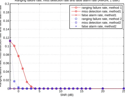
3.11 Ranging failure rate, miss detection rate and false alarm rate in AWGN chan-nel with one ranging user. . . 48

3.12 Ranging failure rate, miss detection rate and false alarm rate in AWGN chan-nel with two ranging users. . . 49

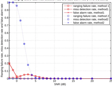
3.13 Ranging failure rate, miss detection rate and false alarm rate in AWGN chan-nel with three ranging users. . . 49

3.14 Average success rate of each user with method 1 in AWGN channel. . . 50

3.16 Ranging failure rate, miss detection rate and false alarm rate in SUI-3 channel

with one ranging user. . . 51

3.17 Ranging failure rate, miss detection rate and false alarm rate in SUI-3 channel with two ranging users. . . 52

3.18 Ranging failure rate, miss detection rate and false alarm rate in SUI-3 channel with three ranging users. . . 52

3.19 Average success rate of each user with method 1 in SUI-3 channel. . . 53

3.20 RMSE of timing offset estimation in SUI-3 channel. . . 53

3.21 Comparison of the failure detection rates under no CFO and CFO=0.1 in SUI-3 channel with one ranging user. . . 54

3.22 Comparison of RMSE of timing offset estimation under no CFO and CFO=0.1 in SUI-3 channel with one ranging user. . . 55

3.23 Comparison of average detection rates under no CFO and CFO=0.1 in SUI-3 channel with three ranging users. . . 55

3.24 Comparison of RMSE of timing offset estimation under no CFO and CFO=0.1 in SUI-3 channel with three ranging users. . . 56

4.1 The SMT310Q carrier board (from [15]). . . 59

4.2 The SMT395 module (from [14]). . . 60

4.3 Functional block and CPU diagram of the DSP [17]. . . 61

4.4 Code development flow for TI C6000 DSP (from [20]). . . 68

4.5 Software-pipelined loop (from [22]). . . 72 5.1 Fixed-point data formats used at different points in the ranging signal generator. 74

5.2 Fixed-point data formats used at different points in the ranging signal receiver. 75 5.3 A part of C code for ranging subcarrier selection and multiplication function. 77 5.4 A part of the assembly code for ranging subcarrier selection and multiplication

function (1/2). . . 78

5.5 A part of the assembly code for ranging subcarrier selection and multiplication function (2/2). . . 79

5.6 Software-pipeline information for ranging subcarrier selection and multiplica-tion funcmultiplica-tion. . . 80

5.7 C code for the straightforward method. . . 81

5.8 The c code for modified method 1. . . 83

5.9 C code for the modified method 2. . . 84

5.10 Ranging failure rate of method 1 in AWGN channel with one ranging user. . 86

5.11 Ranging failure rate of method 1 in AWGN channel with two ranging users. . 86

5.12 Ranging failure rate of method 1 in AWGN channel with three ranging users. 87 5.13 Average success rate of each user with method 1 in AWGN channel. . . 88

5.14 RMSE of timing offset estimation in AWGN channel. . . 88

5.15 Ranging failure rate of method 1 in SUI-3 channel with one ranging user. . . 89

5.16 Ranging failure rate of method 1 in SUI-3 channel with two ranging users. . 89

5.17 Ranging failure rate of method 1 in SUI-3 channel with three ranging users. . 90

5.18 Average success rate of each user with method 1 in SUI-3 channel. . . 90

List of Tables

2.1 OFDMA Uplink Subcarrier Allocation [1], [2] . . . 10

2.2 Cross-correlation Values of Ranging Codes . . . 16

2.3 Cross-correlation Values of Ranging Codes (Continued) . . . 17

2.4 Cross-correlation Values of Ranging Codes (Continued) . . . 18

3.1 System Parameters Used in Our Study . . . 41

3.2 SUI-3 Channel Model . . . 43

4.1 Functional Units and Operations Performed [18] . . . 64

5.1 Code Size and Execution Cycles of PRBS Generation of A Code . . . 85

Chapter 1

Introduction

The IEEE 802.16 Wireless Metropolitan Area Network (WirelessMAN) standard family pro-vides specifications for an interface for fixed and mobile broadband wireless access systems. Among them, the IEEE 802.16-2004 has been proposed to provide last-mile connectivity to fixed locations by ratio links. There are four air interface specifications in 802.16-2004: WirelessMAN-SC, WirelessMAN-SCa, WirelessMAN-OFDM, and WirelessMAN-OFDMA.

Orthogonal frequency division multiple access (OFDMA) can be considered as OFDM based frequency division multiple access. It has been adopted as important physical layer techmiques in many specifications recently because of its good spectral efficiency, robust-ness in the multipath propagation environment, and capability to cope with inter-symbol interference (ISI).

An amendment to 802.16-2004, IEEE 802.16e-2005, considers mobility. It provides en-hancement specifications to the 802.16-2004 to support mobile stations (MS) moving at vehicular speeds and thereby specify a combined fixed and mobile systems.

Our study is about the ranging techniques for the IEEE 802.16e OFDMA PHY. Ranging is a important process for an MS to acquire or adjust transmission parameters to initialize or maintain uplink communications with the base station (BS). The transmission parameters

include timing, power, and possibly frequency offset. In this thesis, we use the term MS and subscriber station (SS) interchangeably.

The following shows the work that we have done.

• Study of ranging-related specifications in IEEE 802.16e.

• Development of the ranging algorithms for transmission and reception of ranging

sig-nals.

• Some simple analysis of the performance of ranging algorithms. • Floating-point simulation in fixed and mobile channels.

• Implementation of the algorithms on Texas Instrument (TI)’s digital signal processor

(DSP) employing the Code Composer Studio (CCS). We also use some techniques to accelerate the execution speed of the programs.

This thesis is organized as follows.

• The ranging techniques in the IEEE 802.16e WirelessMAN OFDMA standard are

introduced in chapter 2.

• Chapter 3 introduces the ranging algorithms, and provides some analysis and

simula-tion results.

• The DSP platform is introduced in chapter 4.

• Chapter 5 discusses the implementation of the ranging process on DSP platform. • The conclusion and some future work are given in chapter 6.

Chapter 2

Ranging-Related Specifications in

IEEE 802.16e OFDMA

The material in this chapter is largely taken from [1] and [2]. First, we give an overview of IEEE 802.16e OFDMA standard and introduce some basic idea regarding OFDMA. Then, we introduce the ranging technique in the specification. This is the main content of this chapter. Other contents in the specification are not our concern and are ignored in this introduction.

2.1

Introduction to IEEE 802.16e

The IEEE 802.16 standard specifies the air interface and MAC protocol for Wireless MAN. Part of it has been dubbed WiMAX (Worldwide Interoperability for Microwave Access) by an industry group called the WiMAX Forum. The mission of the Forum is to promote and certify compatibility and interoperability of broadband wireless products.

The first 802.16 standard was approved in December 2001. It is a standard for point to multi-point broadband wireless transmission in the 10–66 GHz band, with only a line-of-sight (LOS) capability. It uses a single carrier (SC) physical layer (PHY) technique.

ap-proved in 2003 to support non-line-of-sight (NLOS) links, operational in both licensed and unlicensed frequency bands from 2 to 11 GHz. It was subsequently integrated with the original 802.16 and 802.16c standards to create the 802.16-2004 standard (initially code-named 802.16d). With such enhancements, the 802.16-2004 standard has been viewed as a promising alternative for providing the last-mile connectivity by radio link. However, the 802.16-2004 specifications were devised primarily for fixed wireless users.

Mobility enhancements are considered in IEEE 802.16e-2005, which was published as an amendment to IEEE 802.16-2004 in February 2006. It specifies four air interfaces: SC PHY, SCa PHY, OFDM PHY, and WirelessMAN-OFDMA PHY. This study is concerned with the WirelessMAN-OFDMA PHY uplink (UL) in a mobile communication environment.

2.2

Introduction to OFDMA

The basic idea of OFDMA is OFDM based frequency division multiple access (FDMA). In OFDM, a channel is divided into carriers which are used by one user at any time. In OFDMA, each user is provided with a fraction of available number of subcarriers, as shown in Figure 2.1.

OFDMA can also be described as a combination of frequency domain and time domain multiple access, where the resources are partitioned in the time-frequency space, and slots are assigned along the OFDM symbol index as well as OFDM subcarrier index [3].

OFDMA has many advantages. For example, cyclic prefix (CP) can deal with the ISI problem, simple equalization techniques (one-tap equalization) can be used, it provides ro-bustness in the multipath propagation environment, and so on. Due to these many benefits, OFDMA is popular recently and has been adopted as the main physical layer techniques in

Figure 2.1: OFDMA frequency description (3-channel schematic example, from [1], Figure 214).

the IEEE 802.16e standard.

2.3

Definition of Basic Terms and Parameters [1], [2]

We present some basic concepts and definition of some parameters and basic terms of the 802.16e OFDMA PHY in this section.

2.3.1

Definition of OFDMA Basic Terms

In the OFDMA mode, the active subcarriers are divided into subsets of subcarriers, where each subset is termed a subchannel. The subcarriers forming one subchannel may, but need not be, adjacent. The concept is shown in Figure 2.1.

In the following, we introduce some basic terms in the OFDMA PHY. Slot

A slot in the OFDMA PHY is a two-dimensional entity spanning both a time and a sub-channel dimension. It is the minimum unit for data allocation. For downlink (DL) PUSC (Partial Usage of SubChannels), one slot is one subchannel by two OFDMA symbols. For uplink (UL) PUSC, one slot is one subchannel by three OFDMA symbols.

Figure 2.2: Example of the data region which defines the OFDMA allocation (from [1]). Data Region

In OFDMA, a data region is a two-dimensional allocation of a group of contiguous sub-channels, in a group of contiguous OFDMA symbols. All the allocations refer to logical subchannels. A two dimensional allocation may be visualized as a rectangle, such as the 4

× 3 rectangle shown in Fig. 2.2.

Segment

A segment is a subdivision of the set of available OFDMA subchannels (that may include all available subchannels). One segment is used for deploying a single instance of the MAC. Permutation Zone

A permutation zone is a number of contiguous OFDMA symbols, in the DL or the UL, that use the same permutation formula. The DL subframe or the UL subframe may contain more than one permutation zone.

2.3.2

OFDMA Symbol Parameters

Primitive Parameters

The following parameters characterize the OFDMA symbols.

• BW : The nominal channel bandwidth.

• Nused: Number of used subcarriers (which includes the DC subcarrier).

• n: Sampling factor. Its value is set as follows: For channel bandwidths that are a

multiple of 1.75 MHz, n = 8/7; else for channel bandwidths that are a multiple of any of 1.25, 1.5, 2 or 2.75 MHz, n = 28/25; else for channel bandwidths not otherwise specified, n = 8/7.

• G: This is the ratio of CP time to “useful” time, i.e., Tcp/Ts. Derived Parameters

The following parameters are defined in terms of the primitive parameters.

• NF F T: Smallest power of two greater than Nused. • Sampling frequency: Fs = bn · BW/8000c × 8000. • Subcarrier spacing: 4f = Fs/NF F T.

• Useful symbol time: Tb = 1/4f . • CP time: Tg = G × Tb.

• OFDMA symbol time: Ts= Tb+ Tg. • Sampling time: Tb/NF F T.

2.4

WirelessMAN OFDMA TDD Uplink [1], [2]

Since the ranging process is performed in the uplink, we only introduce some basic idea of the uplink and ignore the description of downlink. We describe the frame structure and subcarrier allocation briefly. For more details we refer the reader to [1] and [2].

2.4.1

Frame Structure

In licensed band, the duplexing method may be either frequency-division duplex (FDD) or time-division duplex (TDD). FDD SSs may be half-duplex FDD (H-FDD). In license-exempt band, the duplexing method should be TDD. The system that we implement is a TDD system.

When implementing a TDD system, the frame structure is built from BS and SS trans-missions. Figure 2.3 shows an example. Each frame consists of a DL subframe and a UL subframe. The DL subframe begins with a preamble followed by frame control header (FCH), DL-MAP, UL-MAP and DL bursts. The UL subframe contains a ranging subchannel and UL bursts. In each frame, the transmit/receive transition gap (TTG) and receive/transmit transition gap (RTG) shall be inserted between the DL subframe and UL subframe and at the end of each frame, respectively, to allow transitions between transmission and reception functions.

The parts of the frame that are related to ranging process are the UL-MAP and the ranging subchannel. The relation will be described in later sections.

2.4.2

Subcarrier Allocation

The OFDMA PHY defines four scalable FFT sizes: 2048, 1024, 512, 128. Here we only introduce the 1024-FFT subcarrier allocation which is the most popular choice and is used

Figure 2.3: Example of an OFDMA frame (with only mandatory zone) in TDD mode (from [2]).

in our study.

An OFDMA symbol consists three types of subcarriers:

• Data subcarriers: For data transmission.

• Pilot subcarriers: For various estimation purposes.

• Null subcarriers: No transmission at all, for guard bands and including the DC

sub-carrier.

Subtracting the guard tones from NF F T, one obtains the set of used subcarriers Nused. For

both uplink and downlink, these used subcarriers are allocated to pilot subcarriers and data subcarriers. However, there is a difference between the different possible zones. In PUSC uplink which concern us in this study, each subchannel contains its own pilot subcarriers.

Table 2.1: OFDMA Uplink Subcarrier Allocation [1], [2]

Parameter Value Notes

Number of DC subcarriers

1 Index 512 (counting from 0)

Nused 841 Number of all subcarriers used within a symbol

Guard subcarriers: 92,91 Left, right

TilePermutation Used to allocate tiles to subchannels

11, 19, 12, 32, 33, 9, 30, 7, 4, 2, 13, 8, 17, 23, 27, 5, 15, 34, 22, 14, 21, 1, 0, 24, 3, 26, 29, 31, 20, 25, 16, 10, 6, 28, 18 Nsubchannels 35 Nsubcarriers 48 Ntiles 210 Number of subcarriers per tile

4 Number of all subcarriers within a tile Tiles per subchannel 6

allocation and pilot modulation, but the detailed procedure is not related to our study. Therefore, we only introduce some basic ideas here.

The uplink supports 35 subchannels in the 1024-FFT PUSC permutation. Each trans-mission uses 48 data carriers as the minimal block of processing. Each new transtrans-mission for the uplink commences with the parameters as given in Table 2.1. A slot in the uplink is composed of one subchannel in three OFDMA symbols. Within each slot, there are 48 data subcarriers and 24 pilot subcarriers. The subchannel is constructed from six uplink tiles, each having four successive active subcarriers with the configuration as illustrated in Figure 2.4.

2.5

Ranging Process [1], [2]

There are four kinds of ranging process: initial ranging, periodic ranging, handover ranging and bandwidth-request ranging. The last two kinds are for purposes that are not of our

Figure 2.4: Structure of an uplink tile (from [1]).

interest. The first two kinds, initial and periodic ranging, are important uplink processes to ensure that the signals from all active users arrive at the BS synchronously, so that the orthogonality among the subcarriers in the uplink of OFDMA systems is maintained.

Initial ranging allows an MS joining the network to acquire correct transmission para-meters, such as time offset and transmission power level, so that the MS can communicate with the BS. Following initial ranging, periodic ranging allows the MS to adjust transmission parameters so that the MS can maintain uplink communication with the BS. In this section, we mainly introduce periodic ranging. Note that initial ranging process is similar to periodic ranging.

During the periodic ranging procedure, the MS shall find an periodic ranging interval and acquire needed parameters from the UL-MAP message, as shown in Figure 2.5. Then, it shall transmit a randomly chosen frequency domain ranging code (CDMA codes) on the ranging channel in a randomly chosen ranging time slot.

Since more than one MS may choose the same time slot, the received ranging signal may include several MSs’ ranging information. So, at the receiver side, the BS is required to detect different received ranging codes, estimate the timing offset, power level and possibly frequency offset of each user that transmits a periodic ranging code.

Upon successfully receiving a periodic ranging code, the BS broadcasts a Ranging Re-sponse message (RNG-RSP) that advertises the received periodic ranging code as well as the ranging slot (OFDMA symbol number, subchannel, etc.) where the ranging code has been identified. This information is used by the MS that sent the ranging code to identify the ranging response message that corresponds to its ranging request. The RNG-RSP also contains all needed adjustment and a status notification. The status notification may be success, continue or abort. The MS can know what action should be done next according to the status. We refer the reader to [1] and [2] for more details about the periodic ranging process.

The main subjects of our work are ranging code transmission, ranging code detection and timing offset estimation.

2.6

OFDMA Ranging

The WirelessMAN OFDMA PHY specifies a ranging subchannel and a set of pseudonoise (PN) ranging codes. An example of ranging channel in OFDMA frame structure is specified in Figure 2.3. Subsets of codes should be allocated in the Uplink Channel Descriptor (UCD) Channel Encoding message for the four types of ranging, such that the BS can determine the purpose of the received code by the subset to which the code belongs.

A ranging channel is composed of one or more groups of six adjacent subchannels, using PUSC mode, where the groups are defined starting from the first subchannel. Optionally, a ranging channel can be composed of one or more groups of eight adjacent subchannels, using optional PUSC or adjacent subcarrier permutation mode. We use the former in our study since the system we build is based on the PUSC mode. Subchannels are considered adjacent if they have successive logical subchannel numbers. The indices of the subchannels that compose the ranging channel are specified in the UL-MAP message, as shown in Figure 2.5.

Figure 2.6: PRBS generator for ranging code generation (from [2]).

Users are allowed to collide on the ranging channel. To effect a ranging transmission, each user randomly chooses one ranging code from a bank of specified binary codes. These codes are then BPSK modulated onto the subcarriers in the ranging channel, one bit per subcarrier.

2.6.1

Ranging Codes [1], [2]

The binary ranging codes are the PN codes produced by the PRBS generator described in Figure 2.6, which implements the polynomial generator 1 + x1_{+ x}4_{+ x}7_{+ x}15_{. The PRBS}

generator is initialized by the seed b14..b0 = 0,0,1,0,1,0,1,1,s0,s1,s2,s3,s4,s5,s6 where s6 is the LSB of the PRBS seed, and s6:s0 = UL PermBase, where s6 is the MSB of UL PermBase.

The binary ranging codes are the subsequences of the PN sequence appearing at its output Ck. These bits are used to modulate the subcarriers in a group of six adjacent

(logically) subchannels, which is the so-called ranging subchannel. The bits are mapped to the subcarriers in increasing frequency order of the subcarriers, such that the lowest indexed bit modulates the subcarrier with the lowest frequency index and the highest indexed bit modulates the subcarrier with the highest frequency index. The index of the lowest numbered subchannel in the six shall be an integer multiple of six.

The length of each ranging code is 144 bits. The first ranging code is obtained by clocking the PN generator 144 times as specified. The next code is produced by taking the output of

the 145th to 288th clock instances of the PRBS generator, etc.

There are 256 available codes, numbered 0 to 255. Each BS uses a subgroup of these codes, where the subgroup is defined by a number S, 0 ≤ S ≤ 255. The group of codes will be between S and ((S+O+N+M +L) mod 256).

• The first N codes produced are for initial ranging, obtained by clocking the PRBS

generator 144 × (S mod 256) times to 144 × ((S + N) mod 256) −1 times.

• The next M codes produced are for periodic ranging, obtained by clocking the PRBS

generator 144 × ((N + S) mod 256) times to 144 × ((N + M + S) mod 256) −1 times.

• The next L codes produced are for bandwidth (BW) requests, obtained by clocking

the PRBS generator 144 × ((N + M + S) mod 256) times to 144 × ((N + M + L +

S) mod 256) −1 times.

• The next O codes produced are for handover ranging, obtained by clocking the PRBS

generator 144 × ((N + M + L + S) mod 256) times to 144 × ((N + M + L + O +

S) mod 256) −1 times.

The values of S, N, M, L and O are provided in the UCD Channel Encoding message. Possible values are 0 to 255.

2.6.2

Cross-Correlation of Ranging Codes

As mentioned above, the binary ranging codes are generated by the PRBS generator shown in Figure 2.6. Then the codes are BPSK modulated onto the subcarriers in the ranging channel. We provide some analysis of the cross-correlation of the BPSK modulated ranging codes in this section.

Table 2.2: Cross-correlation Values of Ranging Codes code 0 1 2 3 4 5 6 7 8 9 10 11 12 13 0 144 -8 6 14 -10 18 20 -10 0 -6 28 -8 0 -10 1 144 2 22 10 10 16 -2 20 14 16 -12 -8 6 2 144 12 16 -8 -6 4 14 16 6 6 -26 -16 3 144 8 4 6 8 6 -8 -14 14 -2 -8 4 144 -4 14 12 2 -12 -2 6 -2 12 5 144 22 0 -6 -4 14 -10 14 24 6 144 -2 12 -6 -4 12 -4 6 7 144 6 0 -2 30 -14 4 8 144 6 4 8 4 -14 9 144 -38 -22 -10 -16 10 144 -8 4 2 11 144 -20 2 12 144 -6 13 144

Since the length of each BPSK modulated code is 144 bits, the correlation values are between −144 and 144. Ideally, the code should be orthogonal and the cross-correlation of the codes should be zero. But this is not the case and we find that the codes do not have good orthogonality. We calculate the cross-correlation values of ranging code set for given UL PermBase values. Table 2.2 to 2.4 shows some parts of the result for UL PermBase=0. There are 256 × 256 ÷ 2 = 32640 values since there are a total of 256 codes. Since the total table is too large, we only depict some parts of it.

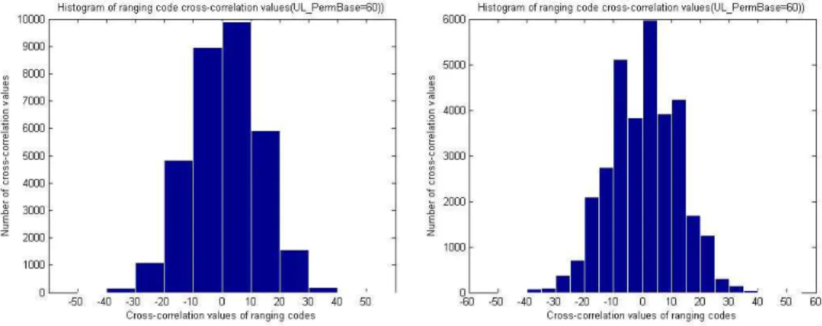
Figures 2.7, 2.8 and 2.9 show the histograms of code cross-correlation values for UL PermBase=0, 30 and 60, respectively. We can conclude that the cross-correlation val-ues are mainly between −20 and 20 and their distribution is little affected by different UL PermBase values.

We also calculate the sample mean and sample variance of the cross correlation values, which are −0.039 and 143.37, respectively.

Table 2.3: Cross-correlation Values of Ranging Codes (Continued) code 14 15 16 17 18 19 20 21 22 23 24 25 26 27 0 16 -10 8 -4 8 2 -2 -20 -10 14 -2 8 -8 -6 1 -20 22 20 12 -8 -10 -2 12 -6 10 6 16 -8 6 2 -6 -8 6 26 -2 -12 4 6 -8 0 -4 -6 6 0 3 -6 -12 -2 14 -2 -12 8 2 4 -4 4 2 18 -8 4 -2 -12 -2 22 -6 12 -20 -10 -4 -8 -8 10 18 8 5 6 0 6 -2 6 16 -8 6 4 -4 32 -6 -6 4 6 -8 14 4 12 4 10 -2 -4 -2 2 14 12 4 -2 7 -6 -4 -2 6 -18 8 -24 2 -8 -20 -4 6 10 -24 8 -24 2 -4 28 -8 -2 6 8 -18 -6 -14 -4 0 6 9 -14 -8 10 -2 -14 -8 8 -22 -32 8 4 -2 14 -12 10 16 2 4 -8 4 -2 10 -8 14 6 -2 -24 -8 6 11 0 6 -16 12 -16 26 -2 -16 10 -14 10 16 -4 6 12 20 6 0 -16 -16 14 14 0 -6 10 6 -4 4 2 13 -2 4 2 -2 2 20 -12 22 0 -16 8 -2 -2 0 14 144 22 4 -4 0 -18 18 -12 -6 30 6 -20 -12 -2 15 144 2 10 18 8 8 10 12 8 12 6 -14 0 16 144 12 -32 -18 -2 4 -6 -10 10 24 -4 -22 17 144 -24 -6 -22 -8 -6 -14 -6 12 -8 10 18 144 6 14 4 2 -10 -10 -12 -8 6 19 144 -32 10 8 -12 12 14 -2 0 20 144 10 -8 4 -4 -10 18 -12 21 144 6 6 2 4 4 -2 22 144 -4 12 -6 -6 20 23 144 0 -6 10 0 24 144 -2 -6 -4 25 144 4 -2 26 144 -10 27 144

Table 2.4: Cross-correlation Values of Ranging Codes (Continued) code 28 29 30 31 32 33 34 35 36 37 38 39 40 41 0 12 0 -10 -16 -4 -10 -16 -4 10 10 2 2 -10 4 1 -4 -8 2 -16 0 -6 16 0 2 -10 -6 -2 10 0 2 10 30 4 10 -2 -20 -2 14 20 -4 0 -4 -8 2 3 14 -2 4 -6 -6 12 6 -14 -4 8 4 12 4 -2 4 26 10 -8 -14 6 0 -2 18 4 -4 -12 24 -20 10 5 -6 -42 -28 -2 14 16 14 2 0 8 12 0 12 -14 6 -8 -8 -22 -12 4 6 8 8 -10 -18 2 -10 10 16 7 14 18 12 -10 -10 -4 2 -6 -4 0 -4 -4 -4 -10 8 -4 12 10 -12 -8 -6 -4 -4 14 26 -6 -2 10 -8 9 6 2 -4 -6 6 -8 -14 6 0 4 -4 0 -8 10 10 -24 16 10 24 -8 -2 24 -4 2 10 2 -2 2 12 11 0 16 2 -16 -4 10 0 8 -14 6 -2 -6 14 12 12 8 -12 -10 -4 20 -2 -8 -20 6 6 -6 -10 2 -36 13 10 -6 -24 -18 -22 20 18 6 -4 -16 12 16 4 2 14 8 -16 -2 16 -16 10 12 -40 -2 10 -10 -22 -18 -12 15 2 -26 20 -2 -10 0 2 -10 -16 0 -12 -16 0 -22 16 -12 -8 -6 20 -4 -18 -4 16 -14 -18 -22 -2 -2 12 17 20 12 -6 20 12 -18 -16 0 -2 -10 -6 -6 -10 12 18 4 -12 -6 4 4 -10 -20 0 10 10 18 2 14 -12 19 14 -10 -20 -14 14 0 -14 18 -4 -4 12 16 20 -14 20 -10 10 8 -10 10 -4 2 -10 12 0 -4 -28 -4 6 21 0 4 -10 0 0 2 -4 8 18 -18 10 -2 -14 -8 22 -6 -10 4 -2 -2 12 22 -10 -4 16 12 -4 -4 10 23 6 10 -16 14 -10 16 -6 -6 0 -8 -4 -12 -4 -18 24 -18 -26 -8 2 14 8 10 6 -20 4 -4 -8 12 -2 25 12 -4 -14 0 12 -18 4 -8 -6 -10 -10 6 14 8 26 8 20 -10 -4 -12 -2 0 16 10 -10 -6 6 -10 -4 27 -6 -10 -4 -2 10 -12 6 -26 12 12 0 12 -8 10 28 144 4 2 -12 -4 -14 -8 -8 18 -18 2 -2 -26 -12 29 144 14 0 32 -14 -28 -4 18 -2 -2 -6 -22 28 30 144 -6 6 -16 2 2 -4 12 12 -24 0 -6 31 144 -4 2 -32 4 -2 10 14 2 18 4 32 144 -6 -4 -12 14 -2 6 10 14 0 33 144 -2 18 -16 -4 8 4 -8 2 34 144 4 -18 2 -14 2 14 0 35 144 -10 -22 2 26 -6 8 36 144 8 4 12 20 -2 37 144 -8 8 12 -2 38 144 -12 4 -10

Figure 2.7: Histograms of ranging code cross-correlation values for UL PermBase=0).

Figure 2.9: Histograms of ranging code cross-correlation values for UL PermBase=60).

2.6.3

Initial-Ranging and Handover-Ranging Transmissions [1],

[2]

The initial ranging codes are used for any MS that wants to synchronize to the system for the first time. Handover ranging codes are used for ranging against a target BS during handover. An initial-ranging transmission is performed using two or four consecutive symbols. In the former case, The same ranging code is transmitted on the ranging channel during each symbol, with no phase discontinuity between the two symbols. A time-domain illus-tration is shown in Figure 2.10. In the latter case, the BS can allocate two consecutive ranging/handover-ranging slots, onto which the MS transmits two consecutive initial-ranging/handover-ranging codes where the starting code shall always be a multiple of 2. A time-domain illustration is shown in Figure 2.11.

The choice of the two transmission ways is indicated in the UL-MAP, as shown in Fig-ure 2.5.

Figure 2.10: Initial-ranging/handover-ranging transmission for OFDMA (from [2]).

Figure 2.11: Initial-ranging/handover-ranging transmission for OFDMA, using two consec-utive initial ranging codes (from [2]).

Figure 2.12: Periodic-ranging or bandwidth-request transmission for OFDMA using one code (from [2]).

2.6.4

Periodic Ranging/Bandwidth-Request Ranging Transmissions

[1], [2]

Periodic ranging transmissions are sent periodically for system periodic ranging. Bandwidth-request transmissions are for Bandwidth-requesting uplink allocations from the BS. These transmissions shall be sent only by an MS that has already synchronized to the system.

To perform either a periodic-ranging or bandwidth-request transmission, the MS can send a transmission in one of two ways: Modulate one ranging code on the ranging subchannel for a period of one OFDMA symbol (a time-domain illustration is shown in Figure 2.12), or modulate three consecutive ranging codes (the starting code shall always be a multiple of 3) on the ranging subchannel for a period of three OFDMA symbols, one code per symbol (a time-domain illustration is shown in Figure 2.13).

The choice of the two transmission ways is indicated in the UL-MAP, as shown in Fig-ure 2.5. Here we choose the former in our study.

Figure 2.13: Periodic-ranging or bandwidth-request transmission for OFDMA using three consecutive codes (from [2]).

2.6.5

Ranging and BW Request Opportunity Size [1], [2]

For CDMA ranging and BW request, the ranging opportunity size is the number of symbols required to transmit the appropriate ranging or BW request code (1, 2, 3 or 4 symbols), and is denoted N1. N2 denotes the number of subchannels required to transmit a ranging code.

In each ranging/BW request allocation, the opportunity size (N1) is fixed and conveyed by

the corresponding UL MAP IE that defines the allocation.

As shown in Figure 2.14, the ranging allocation is subdivided into slots of N1 OFDMA

symbols by N2 subchannels, in a time first order, i.e., the first opportunity begins on the

first symbol of the first subchannel of the ranging allocation, the next opportunities appear in ascending time order in the same subchannel, until the end of the ranging/BW request allocation (or until there are less than N1 symbols in the current subchannel), and then

the number of subchannel is incremented by N2. The ranging allocation is not required to

be a whole multiple of N1 symbols, so a gap may be formed (that can be used to mitigate

interference between ranging and data transmissions). Each CDMA code will be transmitted at the beginning of the corresponding slot.

In our study, we consider 1-symbol periodic ranging transmission so that N1 = 1. And

Chapter 3

Ranging Techniques for IEEE 802.16e

OFDMA

In this chapter, we discuss the ranging techniques for the IEEE 802.16e system. Some existing initial ranging methods have been described in [4]. Here we describe our ranging algorithm, present some analysis and show some simulation results.

3.1

Ranging Signal Processing

Figure 3.1 shows the overall uplink transceiver system. The ranging signal generator and receiver blocks are our main concern. Ranging operation is performed in the frequency domain, that is, before the transmitter IFFT process and after the receiver FFT process.

The algorithms of initial ranging and periodic ranging are similar, but we focus on peri-odic ranging here.

Ranging Signal Generator

Figure 3.2 shows the structure of the ranging signal generator. The tasks here are simple and straightforward. The PRBS generator, whose structure is shown in Figure 2.6, generates the binary ranging code according to the ranging information. The ranging information includes

Figure 3.2: Ranging signal generator.

parameters S, N, M, UL PermBase, subchannel offset and used code number. Then the code is BPSK modulated. Finally, some permutation operation is performed to map the BPSK modulated code to the subcarriers.

Ranging Signal Receiver

The main task here are ranging code detection and timing offset estimation. We do not perform frequency offset estimation in the periodic ranging process. The reason will be described later.

Figure 3.3 depicts the overall structure of the ranging signal receiver system. The inputs to the ranging signal receiver are the ranging information and R(k), which is the received signal after the FFT. The output is a ranging report containing the information of detected codes and estimated timing offsets.

The ranging signal reception is performed on the frequency domain signal R(k). First, the ranging subcarrier selector extracts subcarrier values on which a ranging code may be loaded. Since the length of a ranging code is 144 bits, the length of S(k) is 144 subcarriers. The ranging code generator generates all possible periodic ranging codes. The next step is multiplication of S(k) by each possible ranging code Ci(k). The length of the output M(k) is also 144. After the multiplication, we perform 1024-point IFFT. Since the length of M(k) is only 144, 880 zeros are inserted to the frequency positions before IFFT. The result

after IFFT, U(m), consists of 1024 complex samples. Then the norm operation calculates the norm of U(m). Finally, the norm values are used for code detection and timing offset

estimation. The operation is repeated for each possible periodic ranging code.

The above frequency domain ranging reception algorithm is equivalent to time domain cross correlation. The time domain cross correlation needs 1024 × 1024 complex multi-plications. In our algorithm, using IFFT to perform the equivalent operation needs only 1024 × log₂1024 complex multiplications, which is only 1% of that in time domain cross correlation [5].

The basic concept of our algorithm is shown bellow, assuming presence of additive noise. From DFT theory, we know that a time-domain signal and its DFT are realted by

x[((n − du))N] ←→ WNkdu· X[k]. (3.1)

The received time-domain signal after an additive noise channel is:

r(n) = Cu(n − du) + wA· w(n). (3.2)

Then the frequency-domain signal after FFT is:

R(k) = Wkdu

N · Cu(k) + W (k) (3.3)

where WN=e−j2π/N (here N=1024), wA·w(n) is the added Gaussian noise in the time-domain, W (k) is the equivalent noise in the frequency domain and du is the delay.

The signal after IFFT is:

U(m) = √1 N X k S(k) · Ci(k) · WN−km = √1 N X k [Wkdu N · Cu(k) · Ci(k) · WN−km+ W (k) · Ci(k) · WN−km]. (3.4)

The results after the norm operation are 1024 norm values for each possible delay m, which may be 0 to 1023 samples. The peak value occurs when Ci(k) = Cu(k) and m = du.

The detection and estimation operation contains two steps. First, we decide whether the ranging code is transmitted or not. The decision can be made by two methods. One simple method is setting a single predetermined threshold, h4. If there are any norm value greater

than h4, we say that this ranging code has been transmitted. We denote this method as

method 2. Another method uses three thresholds H, h1 and h2, where h1 is greater than

h2. We calculate the ratio of the mean of norm values greater than h1 to the mean of norm

values smaller than h2. If this ratio (h1/h2) is greater than H, we say that this ranging

code has been transmitted [6]. We denote this method as method 1. The choice of these thresholds and comparison of the two methods are left to later sections.

Second, we perform timing offset estimation when a user is detected, that is, we decide the arrival time of the ranging code. By inspection, we can choose the location of the maximum norm value as the estimated timing offset. But this is not proper in multipath channels. Therefore we use another approach. We let the maximum value of the norm be divided by a number (ht), then we get a new threshold. We choose the first location of norm greater

than this threshold as the estimated timing offset.

3.2

Analysis of the Ranging Algorithm

In this section, we provide some performance analysis of ranging method 2. We do not analyze the performance of method 1 since it involves three thresholds and is too complex. We consider additive white Gaussian noise (AWGN) channel and single-path Rayleigh fading channel. We let the channel link power be 0 dB and let dudenote the delay. We only consider

the case that only one user is doing periodic ranging at this ranging slot. In addition, we assume that timing offset estimation is correct and derive the success rate of ranging code detection. Note that there exists other analysis described in [7].

3.2.1

Case of AWGN Channel

The received time-domain signal after the channel is as given in (3.2), where wA =

q

1

SN R

and

w(n) = wr(n) + j · wi(n) (3.5)

with wr(n) and wr(n) both being Gaussian distributed with zero mean and unity variance.

So wA· wr(n) and wA· wr(n) are also Gaussian distributed with zero mean and variance _{SN R}1 .

Then the frequency-domain signal after FFT is as in (3.3), where

W (k) ≡ Wr(k) + j · Wi(k) = X n wA· w(n) · WNkn = X n wA· wr(n) · WNkn+ j · wA· wi(n) · WNkn. (3.6)

So Wr(k) and Wi(k) are Gaussian distributed with zero mean and variance _{SN R}1 .

The result after IFFT is as given in (3.4). When the multiplied ranging code matches the transmitted one, the result after IFFT should have a peak value, denoted Dp. When the

multiplied code does not match the transmitted one, the value is denoted Ip. Therefore, the

success rate of ranging code detection is

P (successful detection) = P (|Dp| > p h4and |Ip| < p h4) ≈ P (|Dp| > p h4)·PM −1(|Ip| < p h4). (3.7) The former probability is the rate of correct detection and the latter one is the product of the rate of correct rejection. Note that we make an approximation that correct detection and correct rejection are independent. In the following, we derive these two probabilities.

Correct Detection

When the multiplied ranging code matches the transmitted one,

Dp = 1 √ N X k |Cu(k)|2+ Cu(k) · W (k) ≡ RDp+ j · IDp (3.8) where RDp = √1 N { X k |Cu(k)|2+X k Cu(k) · Wr(k)} (3.9) and IDp = 1 √ N X k Cu(k) · Wi(k). (3.10)

Since P_k|Cu(k)|2 = 144 and Wr(k) and Wi(k) are Gaussian distributed with zero mean

and variance 1

SN R, RDp is Gaussian distributed with mean √1441024 = 4.5, and variance

σ2

r

1024.

Similarly, IDp is Gaussian distributed with zero mean and variance σ

2

i

1024. Here σr2 = σ2i =

144 2·SN R.

From [8], we know that R = px2_{+ y}2 _{∼ Ricean(ν, σ) if x ∼ N(ν cos θ, σ}2_{) and y ∼}

N(ν sin θ, σ2_{) are two independent Gaussian distributions and θ is any real number. Here if}

we let θ = 0, ν = 4.5 and σ = _√σr 1024, then |Dp| = q R2 Dp+ IDp2 ∼ Ricean(ν, σ) (3.11) with K = ν2

2σ2. We can further assume K À 1, which is reasonable in our case, so |Dp| is

approximately Gaussian distributed with mean ν and variance σ2_.

Finally, the desired probability can be calculated by

P (|Dp| >ph4) = P (z = |Dp| − ν σ > √ h4− 4.5 σ ), (3.12)

Correct Rejection

When the multiplied code does not match the transmitted one,

Ip ≡ RIp+ j · IIp = √1 N X k [Cu(k) · Ci(k) + Ci(k) · W (k)] = √1 N X k [Cu(k) · Ci(k) + Ci(k) · Wr(k) + Ci(k) · Wi(k)]. (3.13)

The first summation P_kCu(k) · Ci(k), which is the cross correlation of ranging codes,

is often nonzero as shown in section 2.6.2. Therefore we need to consider the effect of this cross correlation term. A simple way is to approximate it as a constant, for instance, 10 or

−10. Another better approach is to approximate it as a random variable. We take the latter

approach. We assume that the cross-correlation term is a Gaussian random variable. Its mean and variance are approximated by the sample mean and variance calculated in section 2.6.2, which are −0.039 and 143.37 respectively. That is, let

X

k

Cu(k) · Ci(k) ∼ N(µc, σ2c) (3.14)

where µc = −0.039 and σ2c = 143.37. Then, RIp is sum of two Gaussian random variable

and thus is also Gaussian:

RIp = 1 √ N X k Cu(k) · Ci(k) + 1 √ N X k Ci(k) · Wr(k) ∼ N(µ1, σ12) ∼ N(√µc 1024, σ2 c + σr2 1024 ) ∼ N(−0.012,143.37 + σ2r 1024 ). (3.15)

And IIp has the same distribution as IDp. IIp = 1 √ N X k Ci(k) · Wi(k) ∼ N(µ2, σ22) ∼ N(0, σ2 i 1024). (3.16) Here we need the probability density function (PDF) of |Ip|2 = R2Ip+ IIp2 , which is the

sum of squares of two Gaussian random variables with different variances. There are two approaches to achieve it. The first is to approximate it by a multiple of a chi-squared distribution that has the correct mean and variance [9]. The second is by transformation of random variables. We take the second approach.

Let

|Ip| = y1+ y2 = RIp2 + IIp2 . (3.17)

We calculate the PDFs of y1 and y2, respectively. Assume that µ1 ≈ 0. Then

f (y1 = R2Ip) = 1 √ 2πσ1 exp{−(− √ y1− µ1)2 2σ2 1 } · | −1 2√y1 | + √ 1 2πσ1 exp{−( √ y1− µ1)2 2σ2 1 } · | 1 2√y1 | = √ 1 2πσ1√y1 exp{− y1 2σ2 1 }. (3.18) f (y2 = IIp2 ) = ... = 1 √ 2πσ2√y2 exp{− y2 2σ2 2 }. (3.19)

Then, let y = y1+ y2 and w = y1 and calculate the joint pdf of y and w.

The corresponding Jacobian is given by

J = ¯ ¯ ¯ ¯ 1 −1_{0 1} ¯ ¯ ¯ ¯ = 1. (3.20)

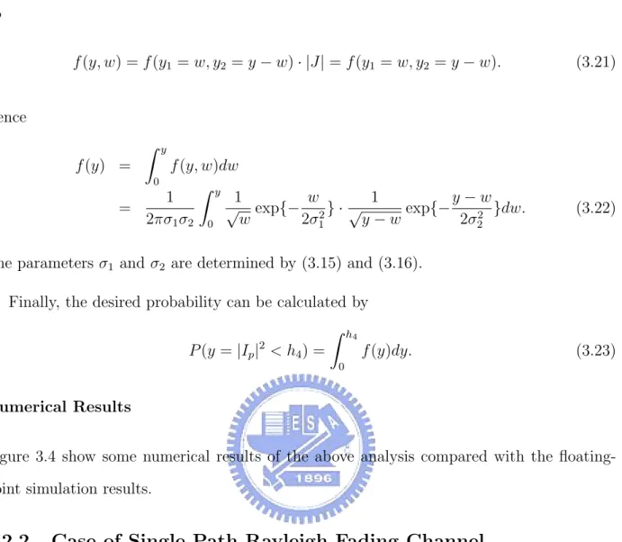
So f (y, w) = f (y1 = w, y2 = y − w) · |J| = f (y1 = w, y2 = y − w). (3.21) Hence f (y) = Z _y 0 f (y, w)dw = 1 2πσ1σ2 Z _y 0 1 √ wexp{− w 2σ2 1 } · √ 1 y − wexp{− y − w 2σ2 2 }dw. (3.22) The parameters σ1 and σ2 are determined by (3.15) and (3.16).

Finally, the desired probability can be calculated by

P (y = |Ip|2 < h4) =

Z _h4

0

f (y)dy. (3.23) Numerical Results

Figure 3.4 show some numerical results of the above analysis compared with the floating-point simulation results.

3.2.2

Case of Single-Path Rayleigh Fading Channel

The time domain received signal after the channel is

r(n) = gF · Cu(n − du) + wA· w(n) (3.24)

where wA and w(n) are the same as that in AWGN case and The fading gain gF is complex

Gaussian with Rayleigh envelope whose PDF is given by

f (|gF| = g) = g σ2 g exp{− g 2 2σ2 g }, (3.25) with σ2 g = 0.4146.

−20 0 2 4 6 8 10 12 14 16 18 20 0.02 0.04 0.06 0.08 0.1 0.12 0.14 SNR (dB)

ranging failure rate

Ranging failure rate (simulation vs. analysis) (AWGN, 1 user) ranging failure rate, method 2 (floating−point simulation) ranging failure rate, method 2 (analysis)

Figure 3.4: Analysis results vs. simulation results in AWGN channel. The frequency-domain signal after FFT is

R(k) = gF · WNkdu· Cu(k) + W (k) (3.26)

where W (k) is the same as that in AWGN case. The result after IFFT is

U(m) = √1 N X k S(k) · Ci(k) · WN−km = √1 N X k [gF · WNkdu· Cu(k) · Ci(k) · WN−km+ W (k) · Ci(k) · WN−km]. (3.27)

Similar to the AWGN case, when the multiplied ranging code matches the transmitted one, the result after IFFT should have a peak value, denoted Dp. When the multiplied code

does not match the transmitted one, the value is denoted Ip. Therefore, the success rate

detection and the second one is the product of the rate of correct rejection. In the following, we derive these two probabilities, too.

Correct Detection

When the multiplied ranging code matches the transmitted one,

Dp = 1 √ N X k gF · |Cu(k)|2+ Cu(k) · W (k) ≡ RDp+ j · IDp. (3.28)

Since gF is a random variable, we calculate the PDF of |Dp| by the following f (|Dp| = x) =

Z _∞

0

f (x|g)f (g)dg, (3.29) where we let |gF| = g whose PDF is as given in (3.25).

In the following we find the conditional probability f (x|g) where

x = |√1 N X k gF · |Cu(k)|2+ Cu(k) · W (k)| = q R2 Dp+ IDp2 (3.30) with RDp = 1 √ N { X k gre· |Cu(k)|2+ X k Cu(k) · Wr(k)} ∼ N(gre√· 144 1024 , σ2 r 1024) (3.31) and IDp = 1 √ N { X k gim· |Cu(k)|2+ X k Cu(k) · Wi(k)} ∼ N(g√im· 144 1024 , σ2 i 1024). (3.32)

Note that gF = gre+ jgim here.

From [8], if we let ν cos θ = 4.5gre and ν sin θ = 4.5gim, we get ν = 4.5g and σ = √σ₁₀₂₄r .

Finally, the desired probability can be calculated by P (|Dp| = x >ph4) = 1 − Z √ h4 0 f (x)dx, (3.33) where f (x) is as given by (3.29) and the value of σ is determined by SNR.

Correct Rejection

When the multiplied code does not match the transmitted one,

Ip ≡ RIp+ j · IIp = √1 N X k gF · Cu(k) · Ci(k) + Ci(k) · W (k) = √1 N X k gF · Cu(k) · Ci(k) + Ci(k) · Wr(k) + Ci(k) · Wi(k) (3.34)

where gF is complex Gaussian with Rayleigh envelope whose PDF is given by (3.25) and

P

kCu(k) · Ci(k) is assumed to be Gaussian distributed with mean µc= −0.039 and variance σ2

c = 143.37. Similarly as in the case of correct detection, we can calculate the PDF of |Ip|

as

f (|Ip| = y) =

Z _∞

0

f (y|g)f (g)dg, (3.35) where for the conditional probability f (y|g),

y = |√1 N X k gF · Cu(k) · Ci(k) + Ci(k) · W (k)| = q R2 Ip+ IIp2 , (3.36) with RIp = √1 N { X k gre· Cu(k) · Ci(k) + X k Ci(k) · Wr(k)} ∼ N(gre√ · µc 1024, σ2 c + σr2 1024 ) ∼ N(−0.0012gre, 143.37 + σ2 r 1024 ) ∼ N(0,143.37 + σ2r_{) (3.37)}

and IIp = 1 √ N { X k gim· Cu(k) · Ci(k) + X k Ci(k) · Wi(k)} ∼ N(gim√ · µc 1024, σ2 c+ σi2 1024 ) ∼ N(−0.0012gim, 143.37 + σ2 i 1024 ) ∼ N(0,143.37 + σ2i 1024 ). (3.38) Again, gF = gre+ jgim here.

So y|g is Rayleigh distributed with σ2 ₌ 143.37+σ2

r 1024 . The PDF is given by f (y|g) = y σ2 exp{− y2 2σ2}. (3.39)

Finally, the desired probability can be calculated by

P (y = |Ip| < p h4) = Z √ h4 0 Z _∞ 0 f (y|g)f (g)dgdy. (3.40) Numerical Results

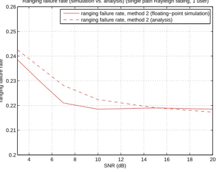
Figure 3.5 shows some numerical results of the above analysis compared with the floating-point simulation results. The analysis results here is less accurate than the AWGN case since we employ some approximation in the derivation.

3.3

Floating-Point Simulation

In this section, we describe our simulation environment first. Then we discuss the penalty of missed detection and false alarm in ranging signal detection. At the end, we show some simulation results and the effect of carrier frequency offset (CFO).

4 6 8 10 12 14 16 18 20 0.2 0.21 0.22 0.23 0.24 0.25 0.26 SNR (dB)

ranging failure rate

Ranging failure rate (simulation vs. analysis) (single path Rayleigh fading, 1 user) ranging failure rate, method 2 (floating−point simulation) ranging failure rate, method 2 (analysis)

Figure 3.5: Analysis results vs. simulation results in single path Rayleigh fading channel.

3.3.1

System Parameters

The important system parameters used in our study are listed in Table 3.1.

We let parameter S = 5, N = 6 and M = 16 in our simulation. That is, there are a total of sixteen possible periodic ranging codes, which are from the twelfth code to the twenty-seventh code generated by the PRBS generator. We simulate up to the situation of three simultaneous ranging users. The codes used by these three users are the twelfth, the fifteenth and the eighteenth code, respectively. We let UL Permbase=0. The timing offsets of the three users are 10, 15 and 7 samples, respectively.

3.3.2

Channel Environments

The simulation is done with AWGN and SUI-3 channels with mobile speed being 60 km/hr. More detailed channel environments are described in the following, which are taken from

Table 3.1: System Parameters Used in Our Study Parameter Value System Channel Bandwidth (MHz) 10

Sampling Frequency (MHz) 11.2

FFT Size 1024

Subcarrier Spacing (kHz) 10.94 Useful Symbol Time (µsec) 91.4

Guard Time (µsec) 11.4 OFDMA Symbol Time (µsec) 102.9

G (Ratio of CP Time to “Useful” Time) 1/8

n (Sampling Factor) 28/25

[10] and [11].

Typical models of the wireless communication channel include additive noise and mul-tipath fading. For channel simulation, noise and mulmul-tipath fading are described as random processes, so they can be algorithmically generated as well as mathematically analyzed. Gaussian Noise

The simplest kind of channel is AWGN channel, where the received signal is only subject to added noise. A major source of this noise is the thermal noise in the amplifiers which may be modeled as Gaussian with zero mean and constant variance. In computer simulations, random number generators may be used to generate Gaussian noise of given power to obtain a particular SNR.

Slow Fading Channel

In slow fading, multipath propagation may exist, but the channel coefficients do not change significantly over a relatively long transmission period. The channel impulse response over

a short time period can be modeled as

h(τ ) = N −1_X

i=0

αiejθi_{δ(τ − τi) (3.41)}

where N is the number of multipaths, αi and τi are respectively the amplitude and the

delay of the ith multipath, and θi represents the phase shift associated with path i. These

parameters are time-invariant in a short enough time period. Fast Fading Channel

With sufficiently fast motion of either the transmitter or the receiver, the coefficient of each propagation path becomes time varying. The equivalent baseband channel impulse response can then be better modeled as

h(τ, t) = N −1_X

i=0

αi(t)ejθi(t)δ(τ − τi). (3.42)

Note that αi and θi are now functions of time. But τi is still time-invariant, because the

path delays usually change at a much slower rate than the path coefficients. The channel coefficients are often modeled as complex independent stochastic processes. If there is no LOS path between the transmitter and the receiver, then each path may be made of the superposition of many reflected paths, yielding a Rayleigh fading characteristic. A commonly used method to simulate Rayleigh fading is Jakes’ fading model, which is a deterministic method for simulating time-correlated Rayleigh fading waveforms. An improvement to Jakes’ model is proposed in [12].

Power-Delay Profile Model

For simplicity in analysis and simulation, the delay τi in the above two models can be

discretized to have a certain easily manageable granularity. This results in a tapped-delay-line model for the channel impulse response, where the spacing between any two taps is

Table 3.2: SUI-3 Channel Model

Relative delay (µs and sample number) Average power

Tap (µs) (4×oversampling) (normal) (dB) (normal scale) (normalized)

1 0 0 0 0 1 0.7061

2 0.4 17 4 -5 0.3162 0.2233

3 0.9 40 10 -10 0.1 0.0706

an integer multiple of the chosen granularity. For convenience, one may excise the initial delay and make τ0 = 0. Often, it is convenient to normalize the path powers relative to the

strongest path. And, often, the first path has the highest average power.

The channel model used here is a modification of the Stanford University Interim (SUI) channel models proposed in [13]. A set of 6 typical channels was selected for the three most common terrain categories that are typical of the continental United States. The scenario of SUI channels are:

• Cell size: 7 km.

• Base station antenna height: 30 m. • Receiver antenna height: 6 m.

• Base station antenna beamwidth: 120◦_.

• Receiver antenna beamwidth: omnidirectional (360◦_{) and 30}◦_. • Vertical polarization only.

3.3.3

Missed Detection and False Alarm Penalty of Ranging

Sig-nal Detection

Missed detection means that a ranging code has been transmitted by a certain MS but the BS does not detect it. In this case, the BS will send a RNG-RSP with continue status but without corrections [1], [2]. Then the MS will need to retransmit a ranging signal. It will do some random backoff and adjust the power level of ranging signal up to PT x IR M AX. The

MS will send ranging signal at next ranging opportunity, that is, at the next UL-subframe which is 5 ms later according to our simulation parameters.

The false alarm means that the BS detects a ranging code that has not been transmitted by any MS. In this case, the BS will redundantly estimate wrong transmission parameters (time, power and possibly frequency offset). Then the BS will broadcast a RNG-RSP with corrections, but this message is redundant and will not be used by any MS.

We compare the effect of missed detection and false alarm. The effect of missed detection is retransmission of ranging signal. The main penalties are retransmission efforts for the MS and more latency to complete the ranging process because next ranging opportunity will be 5 ms later. On the other hand, the effect of false alarm is needless parameter estimation and RNG-RSP transmission. The main penalties are redundant efforts for the BS and the wasted downlink bandwidth for RNG-RSP transmission.

The rates of missed detection and false alarm are affected by the choice of the detection threshold (h4). Since it is difficult to decide which one costs more, we only set the cost of them

to be a certain ratio. We calculate the weighted costs and use them to help us determining the detection threshold. In the following, we provide some examples of weighted costs in the one ranging user case under single-path Rayleigh fading channel. Note that the weighted cost is obtained by missed detection rate × rmd+ f alse alarm rate × rf a, where we set the

1 1.5 2 2.5 3 3.5 4 4.5 5 5.5 6 0.4 0.45 0.5 0.55 0.6 0.65 0.7 0.75 0.8 0.85 0.9 Threshold (h4)

Weighted cost (md:fa=3:1)

Weighted cost with cost of md:fa=3:1, single user single−path fading, method−2

Figure 3.6: Weighted cost for rmd: rf a = 3 : 1.

shows the results for rmd : rf a being 3:1, 2:1, 1:1, 1:2 and 1:3, respectively. We can choose

the best threshold as the one that leads to a minimum weighted cost. Note that the weighted costs do not have large sensitivity to h4.

3.3.4

Simulation Results

Some floating-point simulation results are shown in this section. Note that the signal-to-noise ratio (SNR) used in our simulation means the ratio of the variance of ranging signal samples to that of the noise samples. The detection thresholds h4, h1, h2 and H we have

chosen are 4.3, 3, 1.55, 12. The value of h4 is determined by the weighted-cost method

mentioned in previous subsection. The determination of h1, h2 and H is also based on the

similar idea but is more complex. Thus, we decide them by many times of simulations. In addition, the number of simulation runs are from 2000 to 5000, depending on the simulated case. For simulations with the SUI-3 channel, 2000 runs are enough to observe more than

1 1.5 2 2.5 3 3.5 4 4.5 5 5.5 6 0.35 0.4 0.45 0.5 0.55 0.6 0.65 Threshold (h4)

Weighted cost (md:fa=2:1)

Weighted cost with cost of md:fa=2:1, single user single−path fading, method−2

Figure 3.7: Weighted cost for rmd: rf a = 2 : 1.

1 1.5 2 2.5 3 3.5 4 4.5 5 5.5 6 0.2 0.25 0.3 0.35 0.4 0.45 0.5 0.55 Threshold (h4)

Weighted cost (md:fa=1:1)

Weighted cost with cost of md:fa=1:1, single user single−path fading, method−2

1 1.5 2 2.5 3 3.5 4 4.5 5 5.5 6 0.2 0.3 0.4 0.5 0.6 0.7 0.8 0.9 1 1.1 1.2 Threshold (h4)

Weighted cost (md:fa=1:2)

Weighted cost with cost of md:fa=1:2, single user single−path fading, method−2

Figure 3.9: Weighted cost for rmd: rf a = 1 : 2.

1 1.5 2 2.5 3 3.5 4 4.5 5 5.5 6 0.2 0.4 0.6 0.8 1 1.2 1.4 1.6 Threshold (h4)

Weighted cost (md:fa=1:3)

Weighted cost with cost of md:fa=1:3, single user single−path fading, method−2