ADAPTIVE
MORPHOLOGY
SHORTEST
PATH
PLANNING
BASED
ON ROTATING
OBJECT AND CRITICAL TRANSITION POINT
Soo-Chang Pei, and Ching-Long Tseng
Department of Electrical Engineering, National Taiwan University
No.
1 Sec. 4, Roosevelt Rd.,
Taipei, 10617, Taiwan,
R.
0. C.
Tel.: 886-2-23635251 -321, FAX: 886-2-23671909
E-mail: pei(~~cc.ee.ritu.edu.lw,
tci~r~tstrver..ee.ntu.eciu.
tw
This paper presents a general approach to find the shortest path for a general moving object with rotation and forwardhackward movement among obstacles of ahitrary shapes. We call the object
of finding a shortest path as path planning. By utilizing the cm-
cept of the critical transition point and adaptive path planning, finding a shortest path problem of car-like vehlcles becomes more practical. Moreover, additional efficiency in routing can be db
tained since the critical transition point is used in the confgura-
tion space. Notice that the computatioml complexity is not n-
creased. A car-like vehicle model with forwardhackward driving and turning mechanism is used to validate the performance of the proposed algorithms. Simulation results show that not only the proposed algorithms are successful in various environments, but also these algorithms have good efficiency in computation. Moreover, routing is gained by the help of morphological hory.
Keywords: critical transition point, adaptive path plannirg,
rotation morphology, MMDT.
1. INlRODUCTION
To find a shortest path (path planning) is major and has stimulated considerable interest in modem manufacturing and other high
technology fields of robotics and artificial intelligence. In the
workspace, let B represents the moving object and pe-assigned
orientation forB, to determine whether there is a continuous colli-
sionfree path from a starting point
z,
to an end pointz2
withsome criteria such as minimal cost or constraints ofB.
In general, these algorithms can be divided into two major
classes, one is configuration space method [I], and the another is
compuhtional geometry method [2]. In a word, the configuration
space method can be regarded as adding the geometry of the mov-
ing object aromd the obstacles. That is, in order to create a new space so as to make the vehicle to be viewed as a reference poinf the geometry of the moving object, is essentially set theoretically added around the obstacles. Most the configuration space method has the advantage of easy implementation and less canputational complexity, but cannot solve the complicated cases traditionally. Some approaches use the conventional maphology to obtain the
configuration space for non-rotating objects [I], and recently rota-
tional morphology is used to find the shortest path for rotating
Another approach is to search the original free space directly without transforming the workspace into configuration space by
d W b
PI,
PI.
0-7803-6725-11011$10.00 02001
IEEE
using computational geometry, for solving such kind of problem. Translations are performed along freeways with mtations per- formed at the intersections of freeway [2]. This approach is called computational geometry method. Most the computational geome- try methods have the advantage of being able to solve complex
cases so as to be more close to real world applications, but in-
creases computational complexity if obstacles gather closely. The
causes intractable system sometimes [SI, some limitations, such as
polyhedral assumption etc., so must be added to simplify problem Up to now, a rotational morphological approach is recently proposed to solve the path planning problem [3], thus the compw tational complexity, compared with the previous approaches, can be quite improved while allowing rotations for mving objects. Furthermore, they bring up the idea of the MMDT (Modified Morphological Distance Transformation), which combines the rotational morphology for processing the orientation, forward and
backward movement into consideraticin in path planning [4]. Then
a better path can be found with low computational complexity. In [4], for some special end positions, it cannot find the colli- siorrfree path by only using the algorithm. So in this paper, we
framework [5] to solve such problem; furthermore, adaptive path
planning problems can be solved. Further, we can apply the c m
cept to the 3-D (>Dimensional) cases so as to be more realistic.
2. ROTATIONAL MORPHOLOGY A N D
MMDT
propose an idea of the critical transition point in the previous
2.1. Path Planning by Rotation Morphology
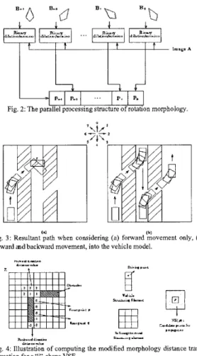
The concept of the rotational morphology is reviewed as follow
[3]: Assume that the full 360' angles are equally divided into N
parts (or directions). For structuring element B , B; denotes the
rotation of B by the degree of 360i/N, for i = 0,1,
...,
N - 1and let y represent 2-D coordinates. Let A is a binary image and B
is a binary structuring element, respectively. Definition 1: The rotational dilation of A byB
( A
c
B ) ( y ) = [A BN - I , A fB BN - 2 ._._, A fB Bi, A fB B o ] ( y ) = [PN - 1, P N - 2...
Pl.PO](y)=
P(Y>
where
Definition 2: The rotational erosion of A by B is a N-bit codeword matrix.
( A e ' B X y ) = [ A 6 BN - I, A Q BN - z ,..., A b B I , A e B o ] ( y ) (2)
Fig. 1 shows an example of rotational erosion. The rotational morphology provides not only the geometric &ape but also the
orientation information. As shown in Fig. 2, the rotational mor-
phology is equivalent to executing N binary morphology modules.
The rotational morphology can be computed in parallel; its com- putational complexity remains the same as the binary molphology.
Property 1; The rotational morphology is translation inva&nt,
where z denotes any 2-D coordinates.
Property 2: Duality,
( A
6
B,)=
( A6
B ) , (3)A'
& E =
( A S B y (4)where A' represents the complement of set A and
i?
repre-sents the symmetric set of B with respect to the origin.
Prope&y 3: Decomposition, for B = C
U
D ,A
6
B = ( A6
C ) U ( A6
D )A eCB=(A k ) U ( A
g o )
(6)2.2. Modified Morphological Distance Transformation
When the configuration space is created by rotational molphology to get FP (Free Position), followed by a distance transformation on these regions with the grown obstacles excluded, and then track back the resultant of distance map from the end point through its neighbors with minimum distance until the beginning point is reached. In order to take forward movement and back- ward movement into consideration at the same time in finding the
shortest path, the MMDT is proposed to combine the rotational
morphology for processing both the orientations, forward and
backward moving information [4]. The new distance transfom-
tion algorithm can overcome the drawback that is allowed only for
forward movements, as shown in Fig. 3.
As shown in Fig. 4, the distance of the beginning points,
which occupied by the VSE (Vehicle-Structuring Element) are set
to
'
0'.
The black regions represent the obstacles in the workspaceZ Assume that moving object is one of the car-like vehicles, and
consider 8direction model as shown Fig. 3 . Then, in order to
c h i n the ondidate points that will propagate from the current
point, one can apply morphology dilation with a 3 x 3
structuring etment at the driving point of the car-like vehicle
marked as current point. To find a collisiowfree path, we must set
this ccnstraint that is not allowed to overlap any pixel of the
obstacles and obey all ncnphysical constraints; one is their directions must be satisfied with the continuos-turning constraint
[ 3 ] , another is the collision-free requirement. Then distance ' 1 ' is
set to these points. The similar procedure can be applied to the corresponding rear points of the dnving position so as to obtain the backward propagation candidate points, which is set distance '-1' correspond to one-step backward movement. All the detailed
steps of MMDT are in [4].
I III.Y...a
Fig. 1: An example of a rotational erosion operation of A by B.
IL-5
Fig. 2: The parallel processing structure of rotation morphology.
(3 WI
Fig. 3: Resultant path when considering (a) forward movement only, (b)
forward and backward movement, into the vehicle model.
?.I.d.,CYI" *.ulu".lu. z D,,... ,YII
E
F
I.l.,..hb.h,,dEl
,".l.', r.l,,il. -.* PL-,.L uli(*: C.,ka.. * ,.,, Y l.,, lua,,..l .I-- B . * . . d b i . , &iu,"",".Fig. 4: Illustration of computing the modified morphology distance trans-
formation for a "/"-shape VSE.
3.
THE PROPOSED PATH PLANNING ALGORlTHM
3.1. Critical Transition Point
When the distance map is obtahed by MMDT for certain begin- ning point, we can find that some points are not able to become the end point; however, it may be a feasible end point from a- other viewpoint. So we modify the original algorithm a little to improve these crcumstances.
For some points of the same distance, two different situations will be existed. One is that passing through certain points cause the end point that cannot be arived from revealing in distance map, but the end point can be actually anived from other view- points. Another is that passing through certain points cause the end point that always cannot be arrived from whatever viewpoints. So starting at the number is smaller in the distance map, the points selected in the path-finding procedure must not only meet con- tinuous turning constraint but also the Bsired end point can be anived when it is viewed from another beginning point. This is the concept of the critical transition point. Using back-traclung
process to find the optimal path of a reference p i n t which is op
erated by morphology operations from the beginning point to the
critical transition point at first, and the second step is to find the
optimal path from the critical transition point to the end point. The
reason of using back-tracking process is that the fore-tracking process has many choices of the beginning point at first Then the
overall directions of the visited points are encoded as a chain code
and the resultant code is sent as the final solution. The detailed
algorithm is described as follows:
-1 In a workspace, all points are viewed as the beginning
points to create all distance maps made by MMDT.
-2. If the desired end point can be anived for the decided te-
ginning point in a workspace, use backtracking process directly
based on distance map made by MMDT.
If it is not met as step 2, repeat step 4 and step 5, and
startmg at distance value is ‘ 1’ to find the critical transition point
For the same value in the distance map, select the point
which must not only meet continuous turning constraint, but also the desired end point must be anived from other viewpoints.
If step 4 can not be satisfied, the testing value is increasing
from ‘ 1’ until celiain point is satisfied with step 4, then go to step
6. Otherwise, rpeat step 4 and step 5. If the distance value in the
distance map is increasing over maximum in a workspace, stop the procedure. It means no critical transition point exists.
When one of the critical transition points is found, use back-tracking process to find the optimal path from the beginning
point to the critical transition point at first And then find the cp
timal path from the critical transition point to the end point.
3.2. Adaptive Path Planning
If the environment is not known in advance or the environment is
changing, path planning must consider this kind of the condition. That is called adaptive path planning. The principle of the solution is to obtain partial information about its environment by viewing it from the present position, and then explore it to gain progres- sively more information until the desired path can be fully
planned. So, based on the concept of the critical transition point,
adaptive path planning problems can be solved. The manner of
adaptive path planning problem is &scribed as below.
SreeL,.
Create the distance map made by MMDT for a decidedbegnning point, the object moves one most suitable pace by back-tracking process and critical transition point algorithm.
Let the present position be the beginning point: create a new distance map made by MMDT based on moving obstacles.
step_?.
Using the new distance map, we decide the next suitable pace of moving object and critical tmsition point finding.Repeat step 2 and step 3 until the moving object anives at
the desired end point
Although the moving object can amve at the end point in a plane (2-Dimensional) in accordance with distance map, we do not guarantee that it has not a collision between the moving object
and the obstacles in altitude. So n the path planning in
3D
case,besides considering common the problem of path planning in a plane, we must pay attention to have no collision between them in altitude at the same time. This is the principle of solving path planning in 3 D case.
Roughly speaking, in configuration space method, the sig- nificant concept is acquired from these two algorithms joined with
3-D case principle in solving all kinds ofpath planning pnlblems.
4. EXPEIRMENTAL RESULTS
AND
DISCUSSIONS
In this section, based on two different shape vehicles within a
field “Z” with size 1 1 x 10 are examined for illustration. One of
the vehicles is a
‘‘I”
-shape car-like vehcle with length ‘ 3’ , theother is non-symmetrical vehicle of “L” -shape with length ‘ 3’
.
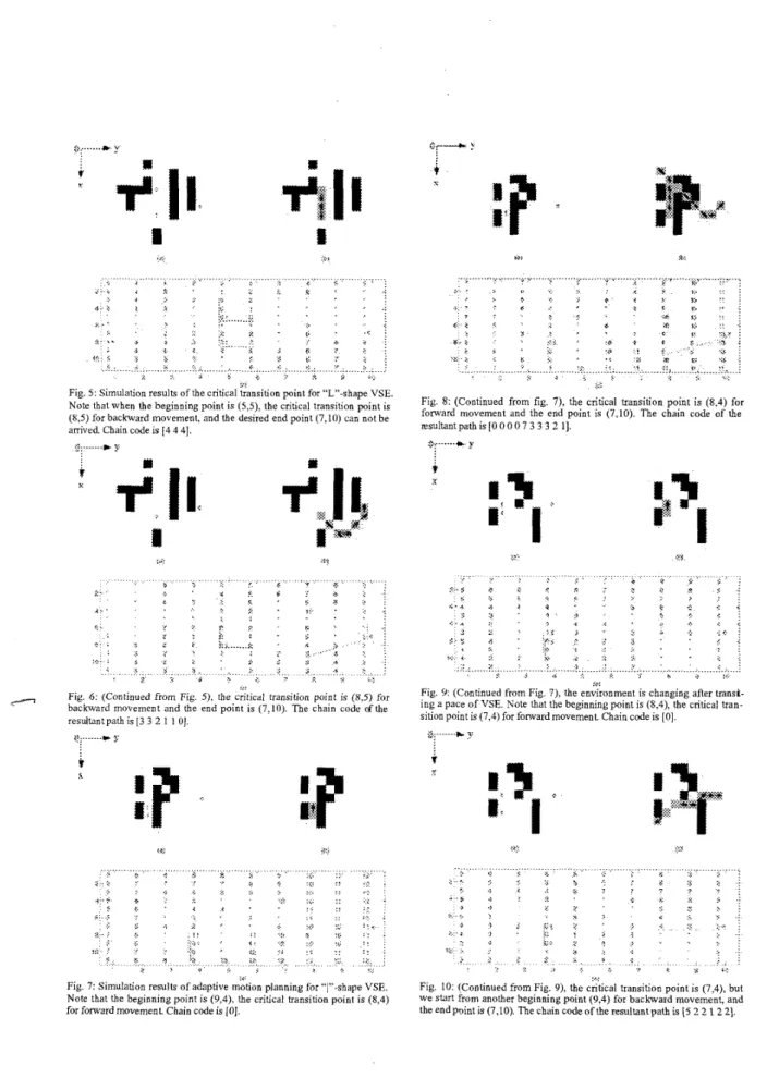
As described above, we find that the end point (7,lO) cannot
be amved when the beginning point is (3,5) with “L,”
-shape
car-like vehicle, as shown in the distance map of Fig. 5. All out- comes of the simulation include the distance map and the results
of backtracking. In Fig. 5 and Fig. 6, we can find that when using
the concept of the critical transition point, the point (7,lO) which
can not be anived shown in Fig. 5 will be anived, the beginning
point is still (3,5) (or the beginning point is (5,5) for backward
moRment). And the critical transition point is (6,5) in this case
(or the critical transition point is (8,5) for backward movement).
There are two circumstances that we must emphasize. One is in considering forward and backward path planning, each one of the front driving point (the upper part of the moving object) and the rear driving point (the lower of the moving object, i.e. its reverse point) ,takes as ‘s’ in figure (the beginning point). Because the
difference between the two cases is just forward movement and
backward movement at first, the way of doing is reasonable. The other is in ‘%‘’-shape car-like vehicle, any a part of moving object amve the desired end point, not necessarily the driving point, we
think the path-findmg to be legitimate, shown as in Fig. 6.
The simulation of adaptive path planning is from Fig. 7 to
Fig. 10. In the first half of the phase, the vehicle is “”-shape
car-like vehicle with length 3. Figs. 7 and 8 represent the shortest
path which contains the concept of the critical transition point
when the environment is shown as the figure, where the beginning
point is (9,4) and the end point is (7,lO). If the environment is
changing as shown in Fig. 9 (or Fig. 10) after transiting a pace of
moving &ject in Fig. 7, the optimal path is shown as Fig. 9 and Fig. 10, which also contains the concept of the critical transition point. Worth to mention is the distinct results between two envi- ronments. It stands for the meaning of “adaptive”.
5.
CONCLUSION
To find the shortest collisionfree p t h among obstacles for arbi-
trary vehicle model, some general algorithms for solving such
problem utilizing the rotational morphology and the modified
mcrphological distance transformation are proposed in this paper. The concept of the critical transition point can solve the problem of the desired end point that can not be anived originally in pre- vious works. The manner of adaptive path planning can find the shortest path adaptively at any time even though the environment
is always changing. However, to join in 1 D case principle of the
path planning, it is more conformed to the circumstance of the real
world. Note that these two algorithms do not increase the c o m p
tational complexity compared to previous algorithms.
6.
REFERENCES
[l] P. L. Lin and S. Chang, “A shortest path algorithm for a non-
rotating object among obstacles of arbitrary shapes,” IEEE
Trans. Syst., Man, Cybern., vol. 23, pp. 825-833, 1993.
[2] 0. Takahashi and R. J. Schiling, “Motion planning in a plane using generalized Voronoi diagrams,” IEEE Trans. Robot.
Automat, vol. 6, pp. 143-150, Apr. 1989.
[3] S. C. Pei, C. L. h i , and F. Y. Shh, “A morphological a p
proach to sholtest path planning for rotating objects,” Paffern
Recognition, vol. 31, no. 8, pp. 1127-1 138, Aug. 1998.
[4] S. C. Pei, C. L. h i , “Forward and backward motion planning
for rotating objects based on morphology,” 11“ IPPR Con-
ference on Comput. Vision, Graphics, Image Processing, pp.
[5] T. LozanePerez and M. A. Wesley, “An algorithm for plarr
ning collkion-free paths among polyhedral obstacles,” Com-
munication of the ACM, vol. 22, no. 10, pp. 550-570, 1979.
346353, W U - h , Taiwan, ROC, Aug. 1998.
5,- ... &. y c-\ i
+./I,
I/.. 2,) ... .;,
, ? . . > . :. :: < $ 5 s : .<,< q . : i y . . .:*,
:t.> I,.
.,
. , > > < .>. 1 : 6.
.< :. Fig. 8: (Continued from fig. 7), the critical transition point is (8.4) for foxward movement and the end point is (7,lO). The chain code of the lesultant path is [0 0 0 0 7 3 3 3 2 11. 0. ...*
y : a n. :> 1 > . _ ' ....
,
: .j ,c..: y ', , i . , :..
... /.,
.2 .: . . . . .a:.
c : . . . < : ... : . . . . . . ... ... :,: 2 - B . . . . . . ... < $ < C ... . A 5 ....
<. . .
.>,:
Fig. 5 : Simulation results of the critical i'ransition point for "L"-shape VSE. Note that when the beginning point is (5,s). the critical transition point is
(8,5) for backward movement, and the desired end point (7,lO) can not be arrived. Chain code is [4 4 41.
... ::.
*
T :d: . ?X .... .... . . . r,.. ' ':, '. : !: x :> j . . ..(. ' ? > .; ' . . . ' & > ~ .! <.
,+.
. . .. .. . . . r .. .> . : :.\. : 1. " - : . . . 2 1 : ..
.
. ..
*
.. i . . . . I. I. .. :). . . ... <._....:...:...I . ? J ., .': ... c i ... j .: ... n :... .> ... :: ... i : I : ....,
...-
Fig. 6 : (Continued from Fig. 5). the critical transition point is (8.5) forbackward movement and the end point is (7:lO). The chain code ofthe resultantpath is [3 3 2 1 1 01.
...
pi C Y
...
Fig. 9: (Continued from Fig. 7), the environment is changing after transt- ing a pace of W E . Note that the beginning point is (8,4), the critical tran- sition point is (7,4) for fonvard movement Chain code is [O].
:: ... a.:
*
i (9: !I:; ... '? 3 8 ;: i ' 7 :< .; 1 :I_ :' <. ' .< ' ...Fig. 7: Simulation results of adaptive motion planning for "/"-shape VSE. Note that the beginning point is (9,4), the critical transition point is (8,4)
for forward movement. Chain code is [O].
... . . I. .> $ >, )I Q i I: :L 5 i :.
...
.; . .: . .> .. \ .: : d 3 :: i 7. .; < .: :. > : 7 7 c : .) :? . , .:,;
,
? : < , . $ ' * " < 7 s ? ' '..' I:. ? > ) . ;< .: .: 3 ' :r:Fig. IO: (Continued from Fig. 9), the critical transition point is (7,4), but we start from another beginning point (9,4) for backward movement, and the end point is (7,lO). The chain code of the resultant path is [ 5 2 2 1 2 21.