Robust Adaptive Array Beamforming with Random Error in Cycle Frequency

(1)

Robust adaptive array beamforming with random

error

in

cycle frequency

Y .-T.Lee and J.-H.Lee

Abstract: By exploiting the cyclostationary properties, the SCORE algorithms presented by Agee

et al. (1990) havc been shown to bc effective in performing adaptive beamforming without rcquiring the direction vector of the desired signal. However, these algorithms suffer from severe performance degradation in the presence of a random error in cycle frequency. The authors first establish a statistical model of the cyclic correlation matrix when the random error exists. According to this statistical model, two robust methods based on the SCORE algorithms are developed to achieve robust adaptive beamforming against random error. Analytical formulas are then derived for evaluating the performance of the proposed methods. Several simulation examples are also presented for confirming the theoretical analysis and showing the effectiveness of the proposed methods.

1 Introduction

Cyclostationarity [ 11, which is a statistical property ex- hibited by most man-made communication signals, corre- sponds to the underlying periodicity arising from carricr frequcncies or baud rates. Recently, a class of spectral self- coherence restoral (SCORE) algorithms has been presented in [2] to deal with blind adaptive beamforming for cyclostationary signals. However, these algorithms suffer from server performance degradation in the presence of cycle frequency error (CFE). Some previous work on thc problem has been reported in [4-81. A statistical analysis presented in [4, 51 shows the cycle leakage through a sinc function due to finite data. On the other hand, two approaches, namely multi-cyclic MUSIC and adaptive-cc cyclic MUSIC, have been presented in [6] to deal with performance degradation due to CFE. However, they cannot tackle the problem efficiently. Variations of the adaptive-cc cyclic MUSIC are explored in [7]. Based on the concept of subintervals, only the cyclic correlation matrices of subintervals are required to reduce the memory requirements and the sensitivity of cyclic MUSIC to CFE. Recently, an efficient technique for coping with the problem of nonrandom CFE in cyclostationarity-exploiting adaptive array beamforming was developed [ 81. Robust adaptive beamforming is achieved by appropriately estimating the actual cycle frequency.

In this paper, two of the SCORE algorithms presented in [2], namely the least-square SCORE (LS-SCORE) and cross-SCORE algorithms, are considered in the presence of random CFE. Based on the central limit theorem, the cyclic correlation matrix with random CFE is equivalent to

0 IEE, 2001

IEE Piweedings online no. 20010425 DUI: 10.1049/ip-rsn:200 10425

Paper first received 21st Februdiy 2000 and in final revised fomi 19th March 2001

The authors are with the Department of Electrical Engineering, Building 2, Nationdl Taiwan University, Taipei 106. Taiwan, Republic of China IEE Pror.-Roclni: Sonar Nuvig,, Pbl. 148, No. 4, Airgist 20Ul

the cyclic correlation matrix computed by using the actual cycle frequency plus a Gaussian random error matrix when the random CFE is an independent sequence. By making use of the ideas originally developed in [9], where two approaches for curing the performance degradation of conventional adaptive beamforming with random steering vector error were presented, two methods based on the LS-SCORE and cross-SCORE algorithms are developed to alleviate the performance degradation due to random CFE. Then, analytic formulas arc derived for evaluating the performance of the proposed methods.

2 Adaptive beamforming using cyclostationarity 2.7 Signal cyclostationarity

For a signal s(t), the cyclic correlation function and conjugate cyclic correlation function are defined as the following infinite-time averages:

and

Ys;.,*cf, 'C) (s(t

+

T / 2 ) S ( t - T / 2 ) d 2 " ) , (2) respectively, where the superscript '*' denotes the complex conjugate. s(t) is then said to be cyclostationary if vss(J 7)

or u,,.(.f; T ) does not equal zero at some time delay z and cycle frequency (CF) J'# 0. Let x(t) denote the data vector received by an array. The cyclic correlation matrix and conjugate cyclic correlation matrix are defined by

R , ( f , T ) = (X(t 4- ' C / 2 ) X " ( t - T/2)e-j2"i), (3) and

respectively, where the superscript ' H ' denotes the conjugate transpose and ' T ' the transpose.

(2)

2.2 SCORE algorithms

Consider an M-clement array excited by a SO1 (signal of interest), J interferers, and spatially white noise. The received array data vector x ( t ) is then given by

J

x(t) = s(t)ad

+

C

!j(t)aj

+

n ( t ) = s(t)ad

+

i(t) ( 5 )

where s(t) and si(t) denote the waveforms of SO1 and the jth interferer, ad and aj are the direction vectors of the SOT

and the jth interferer, respectively, and n(t) is the noise vector. The array output is then given by y(f) = w"x(t), wherc w denotcs the weight vector.

Assume that s(t) is cyclostationary and has a CF equal to

E , but i(t) includes all signals not of interest (SNOIs) and noise and is temporally uncorrelated with s(t). Based on the LS-SCORE algorithm of [2], a cost function is defined as follows:

.j= I

Fl.,(W c ) =

(IA4

- r(t)I2)1. (6) where the reference signal v ( t ) is given by v(t) = c"x(t ~ z)ejZnaf and ( . ) T denotes the average over

the time interval [0, r ] . c is a control vector and is fixed for the LS-SCORE algorithm. The optimal weight vector w I minimising eqn. 6 is given by

where RA, = ( x ( t ) d ' ( t ) ) , and ?Ja) = ( ~ ( t ) r * ( t ) ) ~ are the sample autocorrelation matrix of x ( t ) and the cross- correlation vector of x ( t ) and r(t) computed over [0, T ] , respectively,

To improve the convergence speed of the LS-SCORE algorithm, the cross-SCORE algorithm is proposed by [2], based on maximising the correlation coefficient, which is given by

between y ( t ) and r ( f ) , where u(t) = x ( t - T)e/2nn' is the control signal. It is easy to show that the optimal weight and control vectors maximising eqn. 8 are the dominant eigenvectors of

respectively.

3 Proposed

methods

3. I Statistical model

Assume that

,/=

a

+

Am,, , where ,/and a are the presumed CF and the actual CF, respectively, Aan reprcsents the random cycle frequency error (CFE) at the time instant

nT,, and

r,

is the sampling interval. Substituting t=nT, into eqn. 3, we have the discrete-time version o f the cyclic correlation matrix as

= R,,(a, 7)

+

R , ( f , 7) (10)

where R,(f, z) represents the corresponding error matrix equal to lim,v+m ( 1 / N )

E''

n=l (e-'2nAa,JT~ - l)D,(n, 7 ) and

D,(n,

z)

= x ( n ) f i ( n - z)e-'2ncmTh is independent o f A y n ,

Let { A a n , n = I , 2 , . . . } be an independent random

I94

sequence; the random sequence { ( e-J2nAvtli1T\ ~ I), n = 1 ,

2..

. . } is thus independent. Then, R , ( f; z) equals the sum of infinite independent random matrices and becomes a Gaussian random matrix according to the central limit theorem shown by ([IO], p. 15). As a result, we conclude that when CFE is an independent random sequence, the resulting cyclic correlation matrix is equal to the cyclic correlation matrix computed by using the actual CF plus a Gaussian random error matrix.

3.2 Robust methods based on LS-SCORE algorithm

From eqn. 10, the weight vector shown by eqn. 7 can be expressed as

when Tapproaches infinity. Let R , ( . f ; T ) have zero mean. Then, the vector ar = RJJ z)c is a zero-mean Gaussian random vector since c is a fixed vector. Hence, the log- likelihood function corresponding to a, is given by

wherc C denotcs the covariance matrix of a?.

Accordingly, the role of a, in cqn. 1 1 can be viewcd as the resulting steering error vector due to the random CFE. Using the first method of

[9],

we define a cost function related to a, as

J ( a ) = aHRLJa

+

k(a - & ( , f . T ) c ) ~ ~ - ' ( u - R,yx(,f. T ) C ) (13) where the first term is the inverse of array output power corresponding to the constraint vector a,

R,

is the ensemble autocorrelation matrix ofx(t), and kis apositivcparameter. We obtain the optimal a, and w I , for minimising eqn. 13 as

and

Next, performing the cigendecomposition ofR,, we have I,,$, =

~f

are the eigenvalues of R , in descending order, G:

is the variance of the noise, and e j , i = 1 , . . .

,

M

are the corresponding eigenvectors. The subspaces spanned by

E, = { e l , . . .

,

eJ+I } and E, = {eJ-,

z,

. . .

,

e M } are called

the signal subspace and noise subspace, respectively. Hence, R , can be rewritten as

R ,

=E::,

i i e i e y , where A ,

2 . . .

>

AJ+, > i,,+2 = . .

.

- -

R,, = E,?A,E;

+

E , A , E t (16) wherc A, = diag{i, , . . . ,

A J + I }

and A,, = r7i1. Since

R,(a, z)c = v,,(a, T ) ( U ; C ) U ~ lies in the signal subspace, we use the second method of [9] and define a cost function

J ( a ) = a"E,E:a

+

k(a - R&, T)c)HC-i(a - R , , ( f . T ) C ) as

(17) The optimal a. and w12 minimising eqn. 17 can be easily

obtained as

(18)

a, =

(J

+

1 cE,,E;) - ' R x x ( , f ? z)c

(3)

and

(19)

3.3 Robust methods based on cross-SCORE algorithm

Since R,,, = RXx(J ~)e-'"~' and R;: = R;', we obtain from

eqns. 9 and 10 that the weight vector w, of the original cross-SCORE algorithm equals thc dominant cigenvector of

when T approaches infinity. Substituting R,(a, T) = r,7,r(a, T)U,U; into eqn. 20 and performing some algebraic manipulations, we have

7 2

where a,, = R e ( f ; z)R,;'ad is a Gaussian random vector,

and ae2 = R , ( f , T)R&'RF(J; T ) W , is not a Gaussian random

vector due to the nonlinear operation of R,(J; T ) . Let the elements of R , ( f , T ) be independent idcntically distributed (i.i.d.) white Gaussian random variables with zero mean and variance oz. Then, eqn. 23 becomes a white Gaussian random vector. Assume that 0," is small enough. Thc term

of eqn. 24 is negligible in comparison with the other terms of cqns. 21,22 and 23. Accordingly, we can rewrite eqn. 20 as

where

is a zero-mean white Gaussian random vector. We observe from eqns. 11 and 25 that the weight vectors obtained by using the LS-SCORE and the cross-SCORE algorithms have the similar form in the presence of random CFE. Letting the covariance matrix of a, in eqn. 25 be C = cfZ,

we note from eqns. 15 and 19 that based on the cross- SCORE algorithm it is appropriate to set the optimal weight vector equal to the dominant eigenvector of

where

-1

(Rxx

+

$1) for the first method

I

for the second method

4 Theoretical analysis

Here, wc evaluate the performance in terms of the array output signal-to-interference plus noise power ratio (SINR) for each of the methods proposed above. Consider an M- element uniform linear array (ULA) excited by a S o l , an interferer, and additive white Gaussian noise (AWGN). Substituting R,r.r(a, T ) = r.?,?(c(, ~ ) a , u y and C = a;Z into eqns. 15 and 19, we obtain that the optimal weight vector w l equals R;'R,(J; T ) C = pR;l(ad

+

( 1 / p ) R , ( , f ;

T)C) for the proposed methods based on the LS-SCORE

algorithm, where p = r X 5 ( a , z)(a;'c) and R;' is given by

eqn. 27. In contrast, we have from eqns. 25 and 26 that

w, FX p&'{ ad

+

[y3/(y1

+

y2)]uel } whcn using the cross-

SCORE algorithm, whcre ,U = (y,

+

y 2 ) / A . Moreover, y l

,

y 2

and y3 are given by eqns. 21, 22 and 23, respectively, except that R;' is used instead of R.x;J. As a result, under the situation where the resulting steering error vector is white Gaussian, the optimal weight vector obtained by using the proposed methods developed based on cither the LS-SCORE or cross-SCORE algorithms has a general expression

where

I

ad

l2

= M, and ocae denotes the corresponding

white Gaussian steering error vector with mean zero and covariance matrix oifL We note that ocae is given by

( l / p ) R e ( , f ; T ) C and [ y 3 / ( y 1 + ; ~ ~ ) ] a , , for the proposed

methods bascd on the LS-SCORE algorithm and cross- SCORE algorithm, respectively. Let o : , of, and 0: reprc-

sent the powers of SOI, interference and noise, respectively. From eqns. 16 and 27, we can rewrite R;' as

where

For deriving the output SINR for the proposed methods, we first rewrite a, = c,a,

+

c p ,

+

E , E f a , . Due to the fact

that u ~ E , E ~ u , = u f E , E f a e = 0, we have aya, = ML,

+

(a,HuJc, (30)

{

aya, = (+Z(,)L,

+

Mc, and hcnce M a p l e - ( U J i U d ) f J ~ U ( , c, = M 2 - I Q y U d

l2

(31) 195 IEE PToc-Radar, Sonar Nauig., Vol 148, No. 4, Augurt 2001

(4)

Moreover, because aYR&'ad x 0, we have

ayE,A;'EFa,l 0 and ay{R,,

+

( a 2 / k ) g - ' a d x 0 when of/k is small enough. Therefore, ayE,A;'EFad x 0 for the first aFd second methods. Qn the other hand,

ai'E,EfE,A;'Eyad = 0 and afE,,A;'E{a, = O due to

the orthogonality of E , and E,, . Accordingly, we have

1 0 -

8 -

6 -

where SNR = a:./: and INR = o2/oi. From eqn. 44 in the Appendix, the expectation of S d R l is approximately given by

E(SINR1)

M2<Y2E{l I

+

oPcq 12}SNR

and the output power gain of SO1 is

Simila_ly, because a f E , E f E , i ; ' E y a j = 0 and

ai'E,,A;'Effai

=

0, the output power gain of interference can be expressed by

Moreover, the output power gain of noise is given by

where RG2 = E , A , F ~ E ;

+

E,,A;'Ef and afE,7X,;2EFad

=

c:afE,A;2E.:ad are obtained from eqns. 29 and 32, respectively.

Next, we evaluate afE,s&pEfad and a ~ E s & " E ~ a j for p = 1 and 2 . Consider the case that there onlv exists a SO1 and background noise; -it is easy to show that

E, =en,, c( a d / l / M and A, =

Cs

=Ma:-+ of

+

o:/k for

the first method. Hence, we have afEs,A,'Efad % M<Fp

for the first method. When $ere exists an additional interferer, we note that afE,AFpEfad x

Mt;"

is also valid if

I

af;'uj

1 <<

M. Similarly, we have ayEsATpEfaj M<,?', where

tj

= M.,'

+

01 +

oz/k. Accordingly, the

output SINR obtained by using eqn. 28 for the first method, based on either the LS-SCORE or the cross- SCORE algorithms, is given by

SINR, = PG, x 0," -

PG, x 0,"

+

PG, x ot -

1

+

I ~ S N R

Sinjlarly, we have af;'E&"Efad = Mp;' and

aFE,7A,FpEfa- -Mp;" for the second method, where

ps = Mcr,'

+

C T ~ a n d pj =MO?

+

IT:, From eqn. 45, the

output SINR and the expectation of the output SINR by

81 ...*....*e

...**'::.',

_ _ / - ...___.._... --..

-

...

*

...-

L

'%. -6 I I I I I I I -7 -6 -5 -4 -3 -2 -1 0 1 -8

'

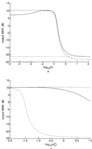
log d a g ) b Fig. 1 exumple I

Output SINR against logarithmic values of k and vz .fir - _ - _ simulation results using first method

* * * * theoretical results using eqn. 36

- theoretical results using eqn. 37

U Against log k

b Against log U:

(5)

using eqn. 28 for the second method, based on either the

LS-SCORE or the cross-SCORE algorithms, are approximately given by SINR, = M2pF21 1

+

occs I'SNR

+

Mp;'(l

+

crcc,

+

cr,c:)

+

o;uFR;2a, c, ( 3 8 ) and EISINR,} - hf2p;2E{

I

1

+

gee,

I

2 ) ~ ~ ~ -

o:E(

I

c, 12M2pJ21NR

+

Mp;'E{(l

+

acts

+

o,c:)]

+

~ ? E ( u ~ ~ R G ~ u , I = M ~ ~ ; ~ s N R /

[

~ p ; 2

+

( M ~ I N R

+

~ ) p ; 2 Ma: M' - 12

+

MCTZ X (39)

1

( M -

2){[k2/(k

+

0 3 2 ~ a ; 4 ~ ( ~ 2 -

I

uFad

12)

M2 -

I

f f U d 12

+

M a ;

+

oc 8 -

z.

6 - z 4 - 3 Q 4 2 - 0 - -2 - -4 1 I I -6 -5 -4 -3 -2 -1 0 1 2 logio(k) a 'og,o(.c', b Fig. 2 example 2

_ _ _ _

simulation results using second method

* * * * theoretical results using eqn. 38

- theoretical results using eqn. 39

a Against log k

b Against log 0:

IEE Proc.-Radar; Sonar Navig., Vol. 148, No. 4, August 2001

Output SINR against logarithmic values of k and CT,' .for

5 Computer simulations

For all simulations, we use a ULA with M = 11 and

interelement spacing = half wavelength of the SOL A SO1 impinging on the array from 5" off broadside has SNR = 0 dB and CF = 2, while an interference with direc-

tion angle 30" off broadside has INR = 9 dB and CF = 3. Moreover, both the SO1 and interference are BPSK signals with rectangular pulse shape and baud rate=0.1. The sampling rate is set to 5. The noise is spatially white Gaussian with mean zero and variance one. All the simulation results of the first four examples are obtained by averaging 1000 independent runs and using 2000 data snapshots for each run. We observe that 2000 data snapshots are enough for computing the correlation inatrkes required for the first four examples. 50 independent runs are averaged for showing the simulation results o f the last example.

Example I : Here, we confirm eqns. 36 and 37 when the optimal weight vector obtained by using the first method, based on either the LS-SCORE or the cross-SCORE algorithm, has the form of eqn. 28. Fig. 1 shows the array output SINR against the logarithmic value of k

with =0.16 and against the logarithmic value of

05

with k=0.01. We observe that the theoretical results

I -20

I

I I I I I I -2.0 -1.5 -1.0 -0.5 0 0.5 1 .o b log,o(.,', Fig. 3 example 3

~. original LS-SCORE algorithm

- first method based on LS-SCORE algorithm

_ - _ _ second method based on LS-SCORF. algorithm n Against log k

b Against log U:

Output SINR uguinst logurilhmic values o j k and U: f o r

(6)

obtained by cqns. 36 and 37 are close to the simulation results. We also note that the mismatch between the theoretical and simulation results increases as of/k increases. This is mainly due to the fact_ that decrcasing,

o:/k improves the approximation a7EsA;'Efad 0 for deriving eqn. 32.

E?cumplc 2: Here, we confirm e q m 38 and 39 when the optimal weight vector obtained by using the second method, based on either the LS-SCORE or the cross- SCORE algorithm, has the form of eqn. 28. The output SINR against the logarithmic value of k with 0; = 0.16, and against the logarithmic value of of with k = 0.001, are plotted in Fig. 2. We observe that the theoretical results obtained by eqns. 38 and 39 are close to the simulation results.

E-xumple 3: This example shows the effectiveness of thc

proposed methods based on the LS-SCORE algorithm. Substituting Rxx(cc, z) = rJS(cc, z ) a d u j into eqn. 11, we obtain r x r ( f )

=&(A

z)c = rFS(cc, z)(a5'c)ad

+

a, that has the form of ad

+

crcae, where oc = l/[r,,(sc, z)(a:c)]. Let

ocar. be a white Gaussian random vector with mean zero and covariance matrix o:I. Fig. 3 depicts the output SINR against the logarithmic valuc of k with of = 0.16 and

- - . . ...~... m

.5c

-20

t

log, a@:) b Fig. 4 u u m p b 4

Outpit SINR against logarithmic values of k and G: f o r

original cross-SCORE algorithm

- first mcthod bascd on cross-SCORE algorithm

.... second method based on cross-SCORE algoritliin

U Againsl log k b Against log U; 198 400 800 1200 1600 2000 -20;

'

number of snapshots a 1 5 1 (iii) I I I I I I I I I I , 0 400 800 1200 1600 2000 number of snapshots b

Oulput SINR against number ojsiiapshots,for example 5 -25 I

Fig. 5

(i) Original algorithm without CFE

(ii) First method based on algorithm with random CFE (iii) Second method based on algorithm with random CF'E (iv) Oiiginal algorithm with random CFE

(I LS-SCOKU algorithm

b Ci-oss-SCORE algorithiii

against the logarithmic value of oz with k=0.01. The simulation results of the original LS-SCORE algorithm are also provided for comparison. We observe that the proposed methods based on the LS-SCORE algorithm can effectively alleviate the performance degradation due to the random CFE by choosing a suitable k. Fig. 3h also shows

that the second method is more effective than the first method, especially for large C T ~ .

Example 4 : Here, we show the effectiveness of the

proposed methods based on the cross-SCORE algorithm. Substituting &(a, z) = rSs(c(, z)adai' into eqn. 10, we obtain R,,(.f;

z)

= rJc(, z)adaf +R,(,f;

z)

that has thc form of adaf

+

oCRe(,f; z), where g c = l/[r& z)]. Let the elements of R,(f; z) be i.i.d. white Gaussian random

variables with mean zero and variance one. The output SINR against the logarithmic value of k with 03 = 0.16 and against the logarithmic value o f 0% with k=0.01 is plotted

in Fig. 4. We observe that the proposed methods provide satisfactory performance when k is appropriately chosen.

Fig. 4h also shows that the second method is more robust than the first method, especially for large oz.

Example 5: We use the same SO1 and interference as those used in the above four examples, except that an additional IEE Proc.-Radac Sonar Navig., Vol. 146, No, 4, August 2001

(7)

BPSK interferer with rectangular pulse shape, direction angle = 40” off broadside, INR = 6 dB, CF = 4, and baud rate=0.1 i s a d d e d . k = 0 . O I , c r ~ = 0 . 1 6 , a n d C = I a r e u s e d by the proposed methods. Fig. 5 depict the output SINR against the number of data snapshots used. In comparison with the results of using the original SCORE algorithms, we observe that thc proposed methods inay provide bettcr pcrformance than the original SCORE algorithms, even in the presence of CFE. This is due to the fact that the term

(cr:/k)l in eqn. 27 for the first method can reduce the finite sample effect if 0: is small and k is appropriately set. The

second method uses the eigenstructurc of the autocorrelation matrix, and hence provides bettcr pcrformance under a siiiall C T ~ and suitable k.

6 Conclusions

This paper has shown that when the random CFE is an independent random sequence, the resulting cyclic correlation matrix equals the cyclic correlation matrix computed by using the actual cyclc frequency plus a Gaussian random error matrix. Rased on the theoretical result, two robust methods in conjunction with the SCORE algorithms have been devclopcd to alleviate the performance deterio- ration duc to random CFE. Moreover, we have cvaluated the performance for each of the proposed methods. The validity of thc theoretical work and the effectiveness of the proposcd methods has also been demonstrated by simulation results.

7 Acknowledgments

This work was supported by the National Science Council under grant NSC88-22 18-E002-027.

References

GARDNEK, W.A.: ‘Cycloslalionarity in communications and signal processing’ (New York, 1994)

AGEE, B.G., SCHELL, S.V, aud GARUNER, W.A.: ‘Spectral self- cohei-ence i-e.;tordl: A new approach to blind adaptive signal cxtraction implification of MUSIC and ESPRIT by exploita- tion of cyclostatioiiarity’, Pmr. IEEE, 1988, 7 6, pp. 845-847 SCHELL, S.V.: ‘Pcrformance analysis of cyclic MUSIC mcthod of direction estimation for cychslalionary signals’, MEE R u m Signal

P,nce.~s.. 1994, 42, (II), pp. 3043-3050

SCHELL, S,V: ‘hsyiiiptotic monicnts of estimated cyclic correlation matrices’, IEEE Pans. Signal Process., 1995, 43, (I), pp. 173-180 SCHELL, S.V; and GAKDNER, W.A.: ‘Progress on signal-selective direction finding’. Procccdings of 5th ASSP workshop on S’ectrm estimation mid modelling, 1990, Rochestcr. NY, pp. 144-148 BIEDKA, T.E., and AGEE, B.G.: ‘Subinterval cyclic MUSIC - robust

DF with error in cycle frequency knowledge’. Procccdings of 25th

Proc. IEEE, 1990,78, pp, 753-767

Asiloma Conference on Signals, systems orid comprriers. 1 Y Y I, Pacific Grovc, C A , pp. 262-266

LEE, J.-H., and LEE, Y.-T.: ‘Kohust adaptive array beamforming for cyclostationaiy signals under cycle frequency error’, IEEE Trum Aiztmnus Propug., 1999, 47: pp. 233-241

I,W, C.-C., and LEE, .I.-H.: ‘Robust adaptive array beamforming under steering vector errors’, IEEE Pans. Antennas Propug., 1997, 45, pp. 168 175

I O GIBRA, 1.N.: ‘Probability and statistical inference for scientists and enginccrs’ (Prcnticc Hall, 1973)

8

9

Appendix

Since thc clcments of a, are white Gaussian random variables with mean zero and variance one, we have

E ( c, ] = E { c , ) = 0 (40) because E{afi‘a,} = E{a;‘ae} = 0. Consequently:

Next, we substitute U , = c,ad

+

cyl

+

E,Ef;’a, inlo E{afR;’a,) and obtain

E : ( u ~ R ; ~ ~ , ) x E{l e, 1’]u;E,A, “ - 2 E, H ad

+

E(

I

c; 12]ayE,A;2E:a,

+

E(a,HEl,A,2E;a,l (43)

It I S easy to show that

E(aFE, 4 , 2 E 5 , ] = tracc{A,2] = ( M - 2)

(

0;

+

-

(44)

when using the first method, and

k’ ( k

+

mt)*

E[a:E,,4,*Epa,} = trace{AL2] = ( M - 2)-

(45) when using the second mcthod.