Automatica, Vol. 25, No. 1, pp, 77-86, 1989 Printed in Great Britain.
0005-1098/89 $3.00 + 0.00 Pergamon Press plc 1989 International Federation of Automatic Control
A Hierarchical Decomposition for Large-scale
Optimal Control Problems with Parallel
Processing Structure*
S H I - C H U N G C H A N G , t T S U - S H U A N C H A N G e : and P E T E R B. L U H §
A hierarchical, time decomposition and coordination scheme for long horizon optimal control problems is suitable for parallel processing and adds a new dimension to results on large-scale dynamic optimization.
Key Words--Dynamic optimization; decomposition and coordination; hierarchical optimization; parallel processing.
Abstract--This paper presents a new method in solving long horizon optimal control problems. The original problem is decomposed along the time axis to form many smaller subproblems, and a high level problem is created that uses initial and terminal states of subproblems as coordination parameters. In such a scheme, the high level problem is a parameter optimization problem. Subproblems are optimal control problems having shorter time horizon, and are completely decoupled so that they can be solved in parallel. It is shown that the two-level problem has the same global optimum as the original one. Moreover, the high level problem is a convex programming problem if the original problem has a convex cost function and linear system dynamics. A parallel, two-level optimization algorithm is then presented, where the the high level problem is solved by Newton's method, and low level subproblems are solved by the Differential Dynamic Programming technique. Numerical testings on two examples are given to illustrate the idea, and to demonstrate the potential of the new method in solving long horizon problems under a parallel processing environment.
1. INTRODUCTION
THERE ARE MANY c o m p u t a t i o n a l m e t h o d s for solving optimal control problems. According to the nature of results, these m e t h o d s can be categorized into three classes: o p e n - l o o p , feed- back, and closed-loop (Polak, 1973). F o r example, m e t h o d s based on dynamic p r o g r a m - ming yield closed-loop solutions while the use of m a x i m u m principle results in o p e n - l o o p solu- tions. As closed-loop solutions are generally * Received 22 October 1986; revised 29 June 1987; revised 24 May 1988; received in final form 1 June 1988. The original version of this paper was not presented at any IFAC meeting. This paper was recommended for publication in revised form by Associate Editor M. Jamshidi under the direction of Editor A. P. Sage.
t Department of Electrical and Systems Engineering, University of Connecticut, Storrs, CT 06268, U.S.A., now at Department of Electrical Engineering, National Taiwan University, Taipei, Taiwan, Republic of China.
Department of Electrical and Computer Engineering, University of California, Davis, CA 95616, U.S.A.
§Department of Electrical and Systems Engineering, University of Connecticut, Storrs, CT 06268, U.S.A.
77
difficult to obtain and p u r e o p e n - l o o p solutions are not satisfactory for practical applications, methods for obtaining solutions with certain feedback properties are typically a d o p t e d (Fin- deisen et al., 1980). T h o u g h there are m a n y existing techniques for solutions of different nature, there have not b e e n m a n y efficient methodologies for solving large-scale problems. As the computational p o w e r increases, such as the availability of faster hardwares and cost- effective parallel processors, etc., the size and scope of p r o b l e m s we want to tackle also grow. E n o r m o u s a m o u n t of research interests have lately b e e n invoked to seek for efficient solution methodologies for large-scale p r o b l e m s by exploiting b o t h p r o b l e m structure and advanced computing techniques, especially the parallelization of algorithms for the application of parallel processing systems.
O n e p o p u l a r scheme in handling large-scale optimization p r o b l e m s , either static or dynamic, is decomposition and coordination: a large p r o b l e m is d e c o m p o s e d , based on p r o b l e m structure, into small s u b p r o b l e m s which can be solved efficiently, and a p r o p e r coordination scheme is created to glue s u b p r o b l e m s t o g e t h e r and to insure the optimality of the solution. Parallelism is usually achieved as a result of decomposition. M e t h o d s such as decomposition by pricing m e c h a n i s m , decomposition by right- hand-side allocation, the generalized B e n d e r s ' decomposition, etc. (Lasdon, 1970; Geoffrion, 1972; Silverman, 1972; Shapiro, 1979) have b e e n developed in the m a t h e m a t i c a l p r o g r a m m i n g literature for static problems. S o m e of t h e m have b e e n applied to dynamic p r o b l e m s by treating systems dynamics as structured constraints and then adopting a static viewpoint
(Lasdon, 1970). The emphasis is on compu- tational efficiency, and the nature of solutions is usually open-loop. On the other hand, for decentralized control applications, methods such as goal coordination, price coordination, inter-
action prediction, etc. (Findeisen et al., 1980;
Jamshidi, 1983; Shimizu and Ishizuka, 1985) have been developed to solve large-scale dynamic optimization problems along the line of decomposition and coordination. Their em- phases are on the dynamic and information feedback aspects. In most of these approaches, decompositions are on state and/or control variables. A parallel dynamic programming algorithm based on state variable decomposition was presented in Scheel (1981~.
For many large-scale optimal control prob- lems, the long time horizon adds another dimension of difficulty. In this paper, we present a scheme that decomposes a long horizon problem into smaller subproblems along the time axis. The initial and terminal states of sub- problems are chosen as coordination parameters. A high level parameter optimization problem is created to determine the optimal coordination. In such a decomposition, subproblems are completely decoupled once coordination para- meters are given, thus they can be solved in parallel.
The basic idea of the new method can be elaborated as follows. Consider a discrete-time, deterministic optimal control problem. If the optimal solution is known, its corresponding optimal state trajectory {x*(k)} can be ob- tained. Let the optimal state trajectory be decomposed into M segments along the time axis, say, segment i starts from stage iT to stage (i + 1)T, where T is a positive integer. The terminal state of segment i, x*((i + 1)T), is also the initial state of segment i + 1. Define subproblem i as the optimization problem over the period [iT, (i + 1)T], having the correspond- ing part of system dynamics and cost function as
the original problem, and x*(iT) and x*((i +
1)T) as its initial and terminal states. From the optimality requirement, an optimal control and its corresponding state trajectory of the original problem in the period [iT, (i + 1)T] must be an optimal solution for subproblem i. Therefore, if the optimal states ( x * ( i T ) } ~ l are given, then subproblems can be solved in parallel since they are decoupled.
The problem then reduces to how to design an efficient algorithm to search for {x*(iT)}~l. To do this, a coordination center is formed at the high level. Its function is to supply subproblems with initial and terminal states. Once subproblems reach their individual solu-
tions, they pass certain information back to the center. The center, based upon the information
received, updates subproblems' initial and
terminal states for the next iteration. The optimal solution can then be obtained iteratively under proper convexity conditions.
In this decomposition, the high level problem is a parameter optimization problem, as its goal
is to find {x(iT)}~l that minimizes the overall
cost. Therefore, many computational methods for parameter optimization can be used to solve it. Similarly, many methods for optimal control can be used to solve low level subproblems. The selection of both methods should be carefully made based on the desired nature of the solution and the computational efficiency of the overall scheme. Note that as the high level is a parameter optimization problem, the solution of the two-level scheme cannot be completely closed-loop even if closed-loop solutions are achieved at the low level. Solutions with a nature between open-loop and closed-loop are generally expected. Note also that state decomposition can be carried out inside each subproblem when
needed. In this sense, our approach is
complementary to existing results.
To illustrate the ideas of our scheme, and to demonstrate the benefit of parallel processing for
long horizon optimal control problems, a
two-level optimization algorithm is developed for the time decomposition of a class of problems with convex, stagewise additive objec- tive function and linear system dynamics. The algorithm consists of two basic components: the Differential Dynamic Programming (DDP) for low level subproblems and the Newton method for the high level (the NM-DDP algorithm). The DDP at the low level explicitly exploits system dynamics, results in variational feedback solu- tions, is efficient for standard optimal control problems (Jacobson and Mayne, 1970; Ohno, 1978; Yakowitz and Rutherford, 1984; Yako- witz, 1986), and generates first and second order derivative information needed for the high level optimization. The Newton method at the high
level generates good search direction for
coordination parameters, has quadratic conver- gence rate near the optimum, and has a special structure suitable for parallel processing as a consequence of time decomposition.
Lacking a parallel processor, our numerical testings were performed on an IBM mainframe with detailed timing and calculation of perform- mance measures (speedup and efficiency, to be discussed in Section 5). These performance measures are good for tightly coupled parallel processing systems where memory is shared among processors and interprocessor com-
Time decomposition for optimal control 79 munications take a negligible amount of time.
For loosely coupled systems where interpro- cessor communication times cannot be ignored,
our measures provide bounds on actual
performances.
The paper is organized as follows. The two-level optimization problem is formulated in Section 2. It is shown in Section 3 that the two-level problem has the same global optimum as the original problem. A sufficient condition for the high level problem to be a convex programming problem is also given. In Section 4, the two-level, parallel NM-DDP algorithm is presented. Section 5 provides numerical testing results on two examples. Concluding remarks are then given in Section 6.
2. THE TWO-LEVEL FORMULATION
Consider the following optimal control
problem:
N - - 1
(P) min J, with J = gN(XN) + ~ gj(x~, U~),
ui i = 0
(2.1) subject to the system dynamics
xi+l =fii(xi, u/), i = 0 . . . . , N - 1, with x0 given, (2.2) and constraints
x ~ X c R , , , and u e U c R " . (2.3) Assume that problem (P) has a finite optimal cost and that N = M T >> 1, where M and T are both positive integers. By specifying the values of {xff,] = 1 . . . M}, we can decompose (P) into M independent, T-stage subproblems as follows.
(P-j) Subproblem j, j = 1 , . . . , M
iT--1
minJj, with J j = ~ g~(xk, uk), (2.4)
Uk k ~ ( j - - 1 ) T
subject to the system dynamics
Xk+l =fk(X,, Uk), (j --
1)T
<_ k <-jT - 1,with x~j_l) T and Xir given, (2.5) and the corresponding constraints of (2.3).
We assume for simplicity that (P-j) has an optimal solution if there exists a feasible sequence of controls that brings the system from
x(j_l)r to Xjr. Denote JT(x(j_l)r, Xjr) as its
optimal cost. If (x(j-1)r, Xjr) is not feasible, i.e. there does not exist a feasible sequence of controls to bring the system from x(j-1)r to xjr, we let J 7 = 00. The low level subproblem (P-j) is therefore well defined for all (x(j-1)r, xjr) • X 2.
Since the solution of (P-j) depends upon x(~-l)r and xjr, the set of variables { X j r } ~ can
be chosen as coordination parameters. A high level problem, called (P-H), is thus created to select the best coordination terms so that the total cost is minimized. That is,
M
(P-H) min J, with J =- ~, J'~(x(i_l)r, xff)
(XMT,... , x r ) ~ X M ] = 1 N--1
= g N ( X N ) "~ E g i ( x ~ , U ~ ) , ( 2 . 6 ) i = 0
where x~' and u~" are solutions of (P-j) with
"Jr __
and x jr =- Xjr, j = 1, M.
X ( j _ l ) T = X ( j _ l ) T • . . ,
The above scheme and the one presented in Chang and Luh (1985) are both time decompo- sition schemes. The major difference is that, instead of modifying subproblems' cost functions as a means of coordination, we choose initial and terminal states of subproblems as coordination terms.
3. ACHIEVABILITY OF OPTIMAL SOLUTIONS In this section, we shall show that problems (P) and (P-H) have the same global optimum. We shall also show that the high level problem (P-H) is a convex programming problem if the original cost function gi is convex, the admissible state space X and the admissible control space U are convex, and the system dynamics f. is linear. Theorem 1. Problems (P-H) and (P) have the same global optimum.
To prove Theorem 1, we first convert problem (P) into a parameter optimization problem. We then utilize the fact that a parameter minimiz- ation problem can be converted into a two-level minimization problem by first minimizing over a subset of parameters and then minimizing over the remaining parameters. Details are given in Appen- dix A.
From Theorem 1, we see that instead of solving the original long horizon optimal control problem (P), we can solve a two-level problem. The high level problem (P-H) is a parameter optimization problem. Low level subproblems (P-j)s are optimal control problems of a shorter time horizon. These subproblems can be solved in parallel, as they are decoupled once { x r } ~ l is set by (P-H).
Though Theorem 1 guarantees that both (P) and (P-H) have the same global optimum, it is not clear whether the two-level formulation changes or creates local optima. In the following theorem, we present a sufficient condition for (P-H) to be a convex parameter optimization problem and therefore have the same optima as (V).
meter optimization problem over the set Xrl if (i) gi(xi, ui) is convex,
(ii) f(xi, ui) is linear, and
(iii) X and U in (2.3) are convex sets.
Proof. Since the cost function in (P-H) is of the additive form as given by (2.6), to prove the theorem, it is sufficient to show that
JV(xu_l)r, xjr) is convex in terms of its arguments. We therefore consider subproblem (P-j). For simplicity of presentation, the subproblem index j is omitted and x(i_~) r is written as x0 in the following proof. Define the set of admissible state and control trajectories
XUA as
X U A ~ ( ( x N . . . X l , UN_ 1 . . . UO) • I N X O N [
(2.2) holds for (XN . . . U0)}. (3.1a) Then define the set of admissible initial and terminal states Xor as
Xor -- {(Xo, xr) [ there exists a trajectory
(xr . . . . , x l , ur-1 . . . Uo)•XUA}. (3.1b) The proof is then reduced to the p r o o f of lemma 1.
Lemma 1. (a) Xov- is a convex set. (b) J*(xo, xr)
is convex over )(or.
Proof. (a) Since fi(x, Ui) is linear, we let
xi+l = Aixi + Biui, i = 0 . . . T - 1, (3.2) where A i e R ~ and B i e R "m. F r o m (3.2), we obtain T - - 1 x~ = ~-~Xo + ~ ~gBgui, (3.3) i = 0 where T - I
(I)~-= I-I Aj and ~ r - ~ - = l .
j=i+l
Let x k, Xo k and (ui k , i = 0 . . . T - l ) , k = 1, 2, denote two sets of quantities satisfying (3.3). Define
xo ° -= 0¢Xo 1 + (1 - c0x~, (3.4a)
x °-= oct,-+ (1 - cr)x2r, (3.4b)
u ° - = c r u ] + ( 1 - c Q u ~ , i = 0 . . . T - l , (3.4c) for an arbitrary o r • [ 0 , 1]. Note that x ° • X ,
x ° • X and u ° • U as X and U are convex sets. We then have
x ° = *_l(a0c~ + (1 - ~)Xo 2) T - - 1
+ i=oE ¢Y~iBi( O{ul +
(1 - cr)u 2) ( 3 . 4 d )T - - I
=f~-I xO+ E tY~iBi uO,
i = 0
which implies (x °, x°r)• Xor. Since this is true for an arbitrary tr • [0, 1], we conclude that Xor
is a convex set.
(b) For a given pair of (Xo k, Xlk), k = 0, 1, 2 as defined in part (a), d e n o t e {x7 k, u *k} as its optimal state and control trajectories and
J*(x~o, x k) its corresponding cost. T o prove that
J*(xo, Xr) is convex in its arguments, we have to show that
J*(x °, x °) <-- trJ*(x~, x~) + (1 - oOJ*(xZo, x2).
(3.5) Define
U(xo, xr) -- {(ui, i = 0 . . . T - 1) • U r [ (14) holds for the given Xo and xr}. (3.6) Note that X and U are convex sets. By letting
= + ( 1 - . 2 ,
and a i = ~ u * l + ( 1 - ~ ) u *z, (3.7) we have (ai, i = 0 . . . T - 1) • U(x °, x°r), and {~i} is the state trajectory for the control sequence {ai}. T h e r e f o r e ,
T - - I
~- o o
J (xo, x r ) = rain g r ( x r ) + ~ gi(xi, ui)
(Uo ... UT-1)~ U(xS,x~ ) i=O
T--1
<--gT(XT) + E gi('~i, tti)
i=0 T - - 1<--gT(xT)+ Z ( gi(x .1, U .1)
i = 0 + (1 - o ( ) g i ( x 7 2 , u 7 2 ) ) = ~r./*(Xo 1, x~) + (1 - oOJ*(xZo, x2). (3.8) The first inequality holds because of (i) above, and the s e c o n d comes from the convexity of g~. The p r o o f is thus completed.4. A PARALLEL PROCESSING ALGORITHM
As formulated in the previous section, the high level problem (P-H) is a p a r a m e t e r optimization problem, and many methods for parameter optimization can be used to solve it. Similarly, many optimal control techniques can be used to solve low level (P-j)s. The selection and integration of methods to solve the two-level problem should be carefully made based on desired nature of results and overall compu- tational efficiency. We present in this section a parallel, two-level algorithm to solve problems without state/control variable constraints, i.e. xl • X = R n and ul • U = R n. O u r emphases are to illustrate the idea of the two-level approach, and to demonstrate its potential for parallel processing of long horizon optimal control problems.
Time decomposition for optimal control 81 (P) are smooth so that all needed derivatives
exist, and that the system is T-stage controllable, i.e. for any given pair of initial and terminal states of subproblem (P-j), there is a feasible solution. Since we are dealing with long horizon problems, T in principle is large. Furthermore, there is no constraint on control variables.
Therefore T-stage controllability is not a
stringent assumption. Newton's method is sel- ected for solving (P-H) as follows:
x T M = x k - [VZJ(xk)]-lVJ(xk), (4.1)
where Xh = (Xlr, - ' .. •, X~r)' and k is the iteration index.
From (2.6), we have
¢r
aJ _ aJ~(xq_or,x/T) 4 aJ/+1(X/r,X(/+t)T)
(4.2) Similarly, the Hessian vEj consists of Hessians of Jj(x(j-1)T, X/r), j = 1 . . . M, and is an M-level block tridiagonal matrix:
bl Cl a2 b2 V2J = a3 0 c2 0 b3 c3 bM-1 aM-1 aM CM-- 1 bM (4.3) where b~ =- a2(J * + JT+l)/ ax2r, aj =- a2(JT_, + J T ) / axq_,)waX/r and c/-=- a2(JT+l + JT+2)/axjrax(/+l)r. Note that both VJj and V2./j can be computed locally by the jth subproblem and passed onto the high level to form VJ and V2j. The problem then reduces to how to find the needed information efficiently while solving low level subproblems. Based on this concern, an extended Differential Dynamic Programming (DDP) technique is adopted at the low level.
The DDP is a successive approximation technique for solving optimal control problems with free terminal states (Jacobson and Mayne, 1970; Ohno, 1978; Yakowitz and Rutherford, 1984; Yakowitz, 1986). It has been extended to problems with fixed terminal states in Chang et al. (1986a), and Chang (1986). It consists of two procedures: backward dynamic programming
and successive policy construction. For a
low-level subproblem (P-j), a backward dynamic programming procedure is applied by taking a
quadratic approximation of (P-j) along a
nominal trajectory, and formulating at each stage a quadratic programming problem in variational terms of control and state variables.
By solving the quadratic programming problem at each stage, coefficients of the linear optimal
variational control and coefficients of the
quadratic variational cost-to-go function are obtained. The successive policy construction procedure uses these control coefficients and the nominal controls to construct new controls forward in time, and to calculate the new cost. If the cost is lower than the nominal one, the nominal trajectory is updated by the new
trajectory. Otherwise the new control is
modified in a specific way till the constructed control yields a cost lower than the nominal one. These forward and backward procedures are carried out repetitively to obtain a convergent solution. The information required by the high level Newton method is readily available from coefficients of the variational cost-to-go function at convergence. A more detailed description of DDP is given in Appendix B. The two-level optimization algorithm with parallel low-level subproblems is depicted in Fig. 1. Note that in the algorithm implemented, the matrix Bjr_~ is assumed to be invertible to simplify the handling of constraints caused by the fixed terminal state. Analysis for the case where Bjr-~ is not invertible can be found in Chang (1986).
To further enhance the parallelism of the algorithm, the block tridiagonal structure of V2j is exploited and the cyclic o d d - e v e n reduction algorithm of Heller (1976) is adopted to find the Newton step
y = [ • 2 J ( X h ) ] - l • J ( X h ) , (4.4)
at the high level optimization. This algorithm is a parallel algorithm that solves the block tridiagonal equation
[V2j(Xh)lY = VJ(Xh). (4.5) To briefly explain the idea of cyclic reduction, let us rewrite (4.5) in block terms defined in (4.3). The jth equation becomes
ajyj-1 + bjyj + cjyj+ 1 = Vj,
j = l . . . . , M , a ~ = c M = 0 , (4.6) where oj is a vector consisting of the components of VJ corresponding to the jth block. Assume for
simplicity that M = 2 m + l - 1 , where m is a
positive integer. There are two basic operations in cyclic reduction: reduction and back substitu- tion. If we multiply equation 2j - 1 by -a2jb~.[1, equation 2/" + 1 by -c2jb2i+l and add them to -1 equation 2j, we can eliminate the odd-indexed, off-diagonal blocks. Picking up blocks associated with the even-indexed unknown y, we form again a tridiagonal equation with 2 m-1 levels of blocks. The procedure is repeated till a one-block equation is obtained. This is the
I
High Level l v,,, J , VZr dt xo given SubprobLem k DDP J; v,,, #," v.~,.,,,V i , j : k - I t k Subprobtern k DDPFIG. 1. The Newton-DDP
JC
v,,r J,;
i , J : M - I , M
Subprobtem M DDP
algorithm with parallel structure.
reduction step. The one-block linear equation is then solved for Y,,+I. The back-substitution step is performed in a reverse sequence of the reduction step. At each stage, the available result is substituted into the block tridiagonal equation constructed at the corresponding stage in the reduction step, and the unresolved variables in the equation can be computed easily and independently for different blocks. This backward procedure continues till the original problem is solved. The algorithm is suited for parallel computation, as many quantities in- volved can be computed independently. Note that the number of processors used is reduced by half after each reduction, and this may not be desirable for the consideration of efficiency. There are other parallel algorithms for solving
block tridiagonal equations (Kowalik and
Kumar, 1985), and the selection of a proper algorithm depends on the architecture of the parallel processor to be used.
5. NUMERICAL RESULTS
As pointed out in Yakowitz and Rutherford (1984), there is no well-established, standard testing problem for large-scale optimal control systems. In this section, two problems with nonquadratic objective functions and linear system dynamics are adopted for the testing purpose. The one level DDP with free terminal state is also tested as a basis for comparison.
As mentioned, numerical testings are per- formed in single precision on an IBM 3084 mainframe computer due to a lack of a paral- lel processor. A user supplied subroutine (pro- vided by UConn Computer Center) is used to time the execution of the algorithm. Two performance
measures, speedup and efficiency (to be
explained later) are obtained assuming no
communication cost among processors. These performance measures are good for tightly
coupled parallel processing systems where
memory is shared and interprocessor com- munications take a negligible amount of time. For loosely coupled systems where interpro- cessor communication times cannot be ignored, our measures provide bounds on actual perform- ances. The timing results listed throughout this section are in units of seconds. Testing results demonstrate the feasibility of the decomposition approach, and the advantage of the algorithm for solving long horizon problems under a parallel processing environment.
Example 1. Cost function:
J = E (xit - a,)Z~, u 2 + u 2
t=l i=1 i=1
+ ~ ~ u, ujt + 100 ~ (xit-ait)2], (5.1)
i=1 j>i i=1
where m = n = 4 , and {air} is an independent, identically distributed random sequence with uniform distribution over the interval [ - 2 , 2]. This cost function is designed to let x, close to air and have small controls. It is convex when magnitudes of x and u are not too large.
System dynamics: A = 0 1 0 0 - 1 0 . (5.2) and B = 1 - 1 0 1 -
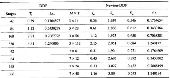
T i m e d e c o m p o s i t i o n for o p t i m a l control TABLE 1. TEST RESULTS FOR TWO PERFORMANCE MEASURES
83 DDP Newton-DDP Stages T1 f.c. M x T lp Sp Ep f.c. 42 0 . 5 9 0.1764597 3 x 14 0.36 1.639 0.546 0.1764654 84 1 . 1 2 0.3430279 3 x 28 0.61 1.836 0.612 0.3430364 168 2 . 2 1 0.7067726 3 x 56 1.12 1.973 0.658 0.7068281 336 4 . 4 1 1.240006 3 x 112 2.15 2.051 0.684 1.240177 42 7 x 6 0.31 1.90 0.271 0.1764609 84 7 x 12 0.43 2.605 0.372 0.3430302 168 7 x 24 0.73 3.027 0.432 0.7068199 336 7 x 48 1.16 3.80 0.543 1.240194 f.c.: final cost/104.
T h e initial state is x0 = [0 0 0 0]', and the initial nominal control is t~it = 0 for all i and t.
Convergence criteria
T h e convergence criteria for the D D P algorithm is of the following form:
IJ~ +1 -- Jkl/Jk <-- r 1. (5.3) T h e convergence threshold 7/ is 0.0001 for the one-level D D P , and T/=0.001 for the D D P in the two-level algorithm. F o r the high level optimization, the criterion is either (5.3) with threshold r / = 0.0001 or IVJI < 0.001.
To m e a s u r e the p e r f o r m a n c e of the algorithm, let T1 be the running time of the one-level D D P , T2 be the total sequential running time of the two-level algorithm, Tp be the corresponding low level parallel running time (to be discussed later), and M be the n u m b e r of processors which is assumed to be equal to the n u m b e r of subproblems. C o m m u n i c a t i o n time is ignored by assuming that either a shared m e m o r y is available, or c o m m u n i c a t i o n time is relatively small. A t the k t h iteration, let tk d e n o t e the longest processing time a m o n g all processors in solving low level subproblems. T h e low level parallel running time Tp is calculated by adding up all the tks. T h e high level c o m p u t a t i o n is assumed to be done by M processors in parallel, and its c o m p u t a t i o n time Th is a p p r o x i m a t e d by
( T 2 - Tp)/M. This a p p r o x i m a t i o n is justified by testing results that T 2 - T p << Tp ( a p p r o x i m a t e l y 1:15), as the high level N e w t o n optimization is much simpler than the low level D D P . T w o p e r f o r m a n c e m e a s u r e s are then a d o p t e d (Heller, 1978). S p e e d u p , defined as Sp =- T1/(Tp + Th),
measures i m p r o v e m e n t in c o m p u t a t i o n time by using parallel processing. On the o t h e r hand, efficiency Ep =-Sp/M, m e a s u r e s how well the processing p o w e r is utilized. Testing results for a sequence of {ait} are given in T a b l e 1.
T A B L E 2. STATISTICS FOR THE TWO PERFORMANCE MEASURES OF EXAMPLE 1 BASED ON MONTE CARLO SIMULATION
M M x T Sp o~s Ep (10 -2) (10 -5) (10 -10) 3 42 1.35 0.293 0.448 3 . 2 5 0 . 3 2 5 0.044 3 84 1.37 0.049 0.455 0.551 0.463 0.037 3 168 1.54 0.074 0.513 0.819 0 . 6 3 8 0.189 3 336 1.56 0.052 0.519 0.579 0.005 0.193 7 42 2.21 0.942 0.315 1 . 9 2 0 . 8 5 4 0.109 7 84 2.70 0.143 0.385 0.292 1.32 0.431 7 168 3.12 0.311 0.446 0.635 0 . 0 1 0 0.041 7 336 3.26 0.118 0.465 0.242 0 . 1 7 8 0.052
Sp: mean of Sp, o2: variance.
Ac: final cost accuracy (percentage difference between one- and two-level final costs relative to the one-level final cost).
T o further study the p e r f o r m a n c e of the algorithm, M o n t e Carlo simulation is p e r f o r m e d by r a n d o m l y generating ai, s. Forty runs are tested for each case. T h e statistics of p e r f o r m a n c e measures are provided in T a b l e 2.
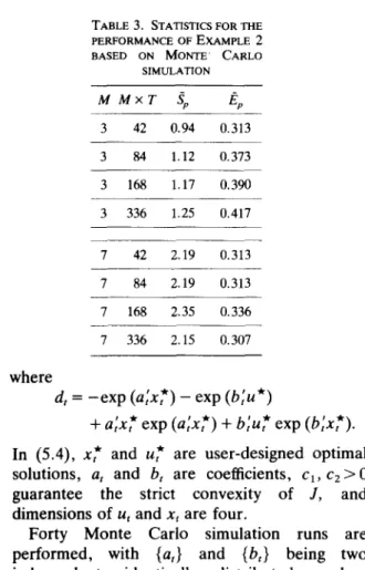
N o t e that the objective function of E x a m p l e 1 is not e v e r y w h e r e convex. T h e following example has a nonquadratic, strictly convex objective function, and its o p t i m a l solution can be specified by the user.
E x a m p l e 2. t T h e system dynamics is the s a m e as in E x a m p l e 1. Stagewise Cost Function is given by
gt(xt, Ut) = exp (a[xt) + exp (b~u,)
' ( a t x t ) -- b,ut exp
- - a t x t e x p ' * ' (btut ) ' *
+ c l ( x , - x , * ) ' ( x , - x,*)
+ c2(u, - u * ) ' ( u t - u * ) + dr, (5.4) t This example and corresponding testing results are prepared by Mr Jian Shi.
TABLE 3. S T A T I S T I C S F O R T H E P E R F O R M A N C E O F E X A M P L E 2 B A S E D O N MONTE' C A R L O S I M U L A T I O N M M × T Sp Ep 3 42 0.94 0.313 3 84 1.12 0.373 3 168 1.17 0.390 3 336 1.25 0.417 7 42 2.19 0.313 7 84 2.19 0.313 7 168 2.35 0.336 7 336 2.15 0.307 where d, = - e x p ( a ~ x * ) - exp ( b ~ u * ) ¢ ~ t ,k t '¢r P "Jr
(b,x, ).
b t u t exp q" (ltX t e x p ( a t x t ) -kIn (5.4), x* and u* are user-designed optimal solutions, a t and b, are coefficients, Cl, c 2 > 0
guarantee the strict convexity of J, and
dimensions of u~ and xt are four.
Forty Monte Carlo simulation runs are
performed, with {at} and {be} being two
independent, identically distributed random
sequences whose components are uniformly distributed over [-0.03, 0.03]. The values of Cl and cz are both 0.0001. The initial state x0 is 0. The optimal control u* is set to be - 2 when t is a multiple of 5, otherwise u* = 0.5. The optimal states are then determined according to the sys- tem dynamics. The initial nominal controls are arbitrarily picked from the interval [-11, 11]. Testing results are given in Table 3.
The above testing results for both examples show that the performance of the two-level algorithm improves as the number of stages increases. This indicates that the temporal decomposition has good potential in tackling long horizon problems under a parallel process- ing environment. However, we also observe that the efficiencies of the 7-processor cases are lower than those of the 3-processor cases. Though Table 2 shows a trend that the 7-processor case could outperform the 3-processor case in the efficiency measure, this is not observed in Table 3. Further investigation on the nature of the algorithm and more numerical testings are needed to draw specific conclusions on the relationship between efficiency and the number of processors.
6. CONCLUSIONS
In this paper, a new method is presented to solve long horizon optimal control problems. Its
key features include decomposition along the time axis, coordination using initial and terminal states of subproblems, and parallel processing to take advantage of the availability of cost-
effective parallel processing facilities. The
two-level approach has nice properties in that
the global optimum is not changed, and
furthermore, the high level problem is a convex programming problem under appropriate con- ditions. A parallel, two-level optimization algo-
rithm for unconstrained problems is then
presented. It employs Newton's method at the high level and the Differential Dynamic Pro- gramming at the low level. The high level solution is open-loop in nature, whereas low level control is in linear variational feedback form. Numerical testing results show that our approach is feasible, the two-level algorithm is suitable for parallel processing, and its perform- ances improve as the time horizon increases.
Note that although the NM-DDP algorithm is designed for unconstrained, convex problems, the two-level problem formulation and its properties (Sections 2 and 3) are addressed based on a larger class of problems. It is therefore believed that the ideas of time decomposition and coordination is promising in tackling many long horizon optimal control
problems. A successful application of the
approach depends on the availability of efficient two-level algorithms. The Newton-DDP com- bination presented here is an example for unconstrained, convex problems. The develop- ment of efficient algorithms for specific appli- cations can be very problem dependent as for many other large-scale optimization techniques. Acknowledgements--This work was supported in part by
NSF Grants ECS-85-13613, ECS-85-04133, ECS-85-12815 and UCD faculty research grant 85-86. A preliminary version of the work was presented at the 1986 American Control Conference (Chang et al., 1986a). The authors would like to thank Mr Jian Shi in providing a test example for the paper.
REFERENCES
Avriel, M. (1976). Nonlinear Programming Analysis and
Methods. Prentice-Hall, Englewood Cliffs, NJ.
Chang, T. S. and P. B. Luh (1985). On the decomposition and coordination of large scale dynamic control problems.
Proc. 24th Conf. on Decision and Control, Fort
Lauderdale, Florida, pp. 1484-1485, December 1985. Chang, S. C. (1986). A hierarchical, temporal decomposition
approach to long horizon optimal control problems. Ph.D. Thesis, Department of Electrical and Systems Engineer- ing, University of Connecticut, Storrs, CT, December 1986.
Chang, S. C., P. B. Luh and T. S. Chang (1986a). A parallel algorithm for temporal decomposition of long horizon optimal control problems. Proc. 1986 Control and Decision
Conf., Athens, Greece, December 1986.
Chang, T. S., S. C. Chang and P. B. Luh (1986). A hierarchical decomposition for large scale optimal control problems with parallel processing capability. Proc. 1986
Time decomposition for optimal control 85
American Control Conf., Seattle, Washington, June 1986,
pp. 1995-2000.
Findeisen, W., F. N. Bailey, M. Bryds, K. Malinowski, P. Tatjewski and A. Wozniak (1980). Control and Coordina-
tion in Hierarchical Systems. John Wiley, New York. Geoffrion, A. M. (1972). Generalized benders' decomposi-
tion. J. Opt. Applic., 10, 237-260.
Heller, D. (1976). Some aspects of the cyclic reduction algorithm for block tridiagonal linear systems. S I A M J.
Numer. Anal., 13, 484-496.
Heller, D. (1978). A survey of parallel algorithms in numerical linear algebra. S l A M Rev., 20, 740-777. Jacobson, D. and D. Mayne (1970). Differential Dynamic
Programming. Elsevier, New York.
Jamshidi, M. (1983). Large-scale Systems. North-Holland, New York.
Kowalik, J. S. and S. P. Kumar (1985). Parallel algorithms for recurrence and tridiagonal equations. In J. S. Kowalik (Ed.), Parallel M I M D Computation: H E P Supercomputer
and Its Applications. MIT Press, Cambridge, MA.
Lasdon, L. S. (1970). Optimization Theory f o r Large
Systems. Macmillan, London.
Ohno, K. (1978). A new approach to differential dynamic programming for discrete time systems. I E E E Tram. Aut.
Control, AC-23, 37-47.
Polak, E. (1973). A historical survey of computational methods in optimal control. S l A M Rev., 15, 553-583. Sage, A. P. and C. C. White, III (1977). Optimum Systems
Control (2nd ed.). Prentice-Hall, Englewood Cliffs, NJ.
Scheel, C. (1981). Parallel processing of optimal control problems by dynamic programming. Inf. Sci., 25, 85-114. Shapiro, J. F. (1979). Mathematical Programming, Structures
and Algorithms. John Wiley, New York.
Shimizu, K. and Y. Ishizuka (1985). Optimality conditions and algorithms for parameter design problem with two-level structure. I E E E Tram. Aut. Control, AC.30, 986-993.
Silverman, G. (1972). Primal decomposition of mathematical programs by resource allocation, Ops Res., 20, 58-93. Yakowitz, S. (1986). The stagewise Kuhn-Tucker condition
and differential dynamic programming. I E E E Tram. Aut.
Control, AC-31, 25-30.
Yakowitz, S. and B. Rutherford (1984). Computational aspects of discrete-time optimal control. Appl. Math.
Comput., 15, 29-45.
APPENDIX A: PROOF OF T H E O R E M 1 To show that problems (P) and (P-H) have the same global optimum, we shall first examine the original problem (P). In (P), an admissible control sequence {ui, i = 0 . . . N - 1 } generates an admissible state trajectory. The optimization can therefore be thought of as being carried out over all possible pairs of admissible controls and corresponding state trajectories. Let us define the set of admissible state and control trajectories XUA as
XUA ~ ( ( X N . . . X l ' UN 1 .. . . . UO) e X N X U N I (2.2) holds for (XN . . . U0)}, (A.1)
then problem (P) is equivalent to the parameter optimization problem (P)' defined below
N - - I
(P)' min J, with J = gN(XN) + ~ , g~(x~, U~).
(XN,...,uo)eXUA i = 0
(A.2)
It is well known that a parameter minimization problem can be converted into a two-level minimization problem by first minimizing over a subset of the parameters, and then minimizing over the remaining parameters. To apply to problem (P)', let us first define the set of all admissible state trajectories XA as
XA =- {(XN . . . Xl) I there exists a
(XN . . . XA, UN--I . . . UO) ¢ X U A } . (A.3)
Let us also define the set of admissible controls for a given admissible state trajectory (XN . . . X 0 as
Ualx(XN . . . xl)
( ( U N _ 1 . . . UO) I (XN . . . X 1, UN-1 . . . UO) E X U A } .
(A.4) Problem (P)' is then equivalent to the following two-level problem (P-H)':
(P-H)' min min J,
(XN,...,Xl)~X A (UN-I,...,uo)~UAIx N--I
with J ~ gN(XN) + ~ gi(xi, ul). (A.5)
i = 0
In (P-H)', we choose all state variables as high level decision variables. If the set (x/r, j = 1 , . . . , M} is chosen instead, we obtain (P-H) in (2.6) by following the same arguments. Note that in this case, the high level decision variables {x/r } are to be chosen from the following feasible set:
X n =- {(X~T, X(M-t)T . . . Xr) [ there exists a
(XN, XN_ t . . . Xl) e X A } . (A.6)
APPENDIX B: DIFFERENTIAL DYNAMIC PROGRAMMING WITH FIXED TERMINAL STATES
Consider a subproblem (P-j):
iT-1
Jj(X(i_I)T, XjT ) ~ rain ~ gk(Xk, Uk) (B.1)
uk k ~ ( j - l ) T
subject to Xk+ 1 = AkX k + BkU k, k = (j - 1)T, . . . . j T - 1, and xti_OT and XjT given. (B.2) Let {ti k, k = (j - 1)T, . . . . ]T - 1} be a given set of nominal controls, and {-~k, k = (j - 1)T, . . . . j T } be the correspond- ing state trajectory. By taking the Taylor series expansion of the above objective function at the last stage, we formulate an approximate linear quadratic problem:
VjT_I(6XjT_I, 6XjT ) ~ min gjT_I(6XjT_I, 6UjT_I) , (B.3)
6ujT--1
with
=- tSX}T_IC/T_t6XiT_ , + 6U;T_,D/T_tt$XiT_ 1
+ au;~_~en-_lau/,-_, + ~,-_,ax/~_, + ~/r_,au/~_,.
(B.4) subject to 6x/r =A/r_16x/r_l + B/r_16u/r_l. (B.5) The above approximate problem is a Quadratic Program- ming (QP) problem (Avriel, 1976) with linear equality constraint, where 6X/T and 6x/r_l are treated as given terms in the problem. The solution of the above QP problem is determined by the nature of the equality constraint (B.5). To convey main ideas, we assume that BiT_ ~ is invertible to simplify the handling of constraints caused by fixed terminal state. Analysis for the case where BiT_ ~ is not invertible can be found in Chang (1986). When B~-T~_~ exists, there is no need for QP. The unique solution is obtained by solving
(B.5):
* __ --1 --1
6UiT- 1 -- B i t - t 6xjr - B / r - 1A/r- 16x/r - 1
=-- % r - 1 + fljr-16XjT-1 + Yjr-16x/r-1, (B.6) where otjr_ l, fljr-1 and Yjr-1 are called control coefficients. Substituting this solution into (B.4), the cost-to-go function is then of the following form:
^
V/r-l(GX/r-l, 6XjT--,) = t~X~r_iP/T_16XiT_ 1 + 6X;T_,QjT_16XiT + 6x/rRjr-ltSXiT+ S/T-, 6 x / r - , + Wit_, 6X/T + O/T_ 1 , ' (e.7)
where P, Q, R, S, W and 0 are appropriate coefficients. For an intermediate stage k, ( j - 1 ) T < - k < _ j T - 2 , by
applying quadratic approximation to gk, we have
fZk(6Xk, ~XjT)=--min [~k(6Xk, ~Uk)+ fZk+~(~Xk+l, 6Xir)], tSu k
(B.8)
subject to 6Xk+ 1 = A , b x k + BkbU k. (B.9) By assuming that lT"k+l(6Xk+ l, 6X/T) is in a quadratic form
similar to (B.7) and by subsmuting (B.9) into it, an unconstrained quadratic optimization problem is obtained:
Vk( 6Xk, 6xjr) = min [ 6x'kCk6x k + 6u'kDkbX k &u k
+ 6u'kEkt~Uk + Fk(OXjr)6X k + Gk(6Xl~r)bU ~ + 0k+l], (B.10)
where F and G are affine functions of 6x r. The optimal
solution again has the following affine form:
6u~ = o: k + flk6Xk + )'k6XjT, (B.11)
and 17', turns out to be a quadratic function of 6x k and 6Xjr.
Performing above steps backwards in time along the
nominal trajectory, control coefficients ok, /~k and Yk for all
stages can be found. Since (B.10) is an approximation, a successor policy construction step is needed to guarantee that the actual cost associated with constructed controls is less than the original nominal cost. This step proceeds by letting
uk(e) = uk + cock + flk(x~ - xk), (B. 12) and
Xk+l=AkXk + Bkuk(¢), k = ( j - 1 ) T , . . . . i T - 1 . (B.13) The initial value of e is one and the corresponding cost is evaluated. If the cost is lower than the nominal cost, the new policy is used to update the nominal trajectories. Otherwise, e is reduced by half till the constructed policy yields a cost lower than the nominal. The backward approximation and forward policy construction procedure are repeated until convergence is achieved. Since
V(I_I)T(~X(j_I)T,
~XjT ) is aquadratic approximation of the variation of J ~ with respect
to 6x~j_l) r and 6xjr, the gradient and Hessian of the
low-level optimal cost with respect to 6x<j ~)r and 6xj. r are