國 立 臺 中 教 育 大 學 教 育 測 驗 統 計 研 究 所 理 學 碩 士 論 文
指導教授:郭伯臣 博士
統計學習方法
在高維度資料分類上之應用
(Statistical learning methods for high
dimensional data classification)
研 究 生:黃 志 勝 撰
Abstract
For supervised classification learning, there are high correlations between the parametric estimations of statistical learning and number of training sample. The larger number of training sample has the more accurate estimation of parameter in the statistical estimation. However, for the high dimensional data classification problem, the number of training sample is limited to the small size on account of that the sample is not easy to collect, and the following problem is ‘‘small training sample size but high dimension’’ problem, and hence, Hughes phenomena, also call the curse of dimensionality, always occurs. Recently, support vector machine (SVM) is shown it provides a great effect on alleviating sample size and high dimensionality concerns, and robustness to Hughes phenomena. The most important factor in SVM is kernel function, but it’s too difficult to find a proper kernel function directly for each dataset. Hence, this thesis presents an automatic algorithm to choose a proper kernel function for SVM. However, there is another problem in the hyperspectral image classification task, it’s training sample come from different land-cover classed, but have very similar spectral properties. In order to overcome this situation, we develop a novel spatial-contextual support vector machine (SCSVM) in the hyperspectral image classification issue. Experiment results show this automatic algorithm has the generalized ability to choose a proper kernel function, and SCSVM has a great improvement in hyperspectral image classification.
Keyword: statistical learning, Hughes phenomena, support vector machine, spectral information, spatial information.
摘 要
在監督式分類學習下,統計學習方法的參數估計往往和訓練樣本是相輔相成 的,訓練樣本數越多在參數的估計上就越能精準的估計;然而,在進行高維度資 料分類時,樣本取得不易、成本過高,導致在進行高維度資料分類時會造成小樣 本高維度的問題發生,所以在利用傳統的統計方法進行分類時常會 Hughes 現象 或是所謂的維度詛咒,造成辨識率不佳的情況。許多研究顯示出支撐向量機為一 種完善且有效可以直接解決 Huhges 現象的分類器,而控制支撐向量機分類效能 的主要因素為kernel 函數,因此本研究將針對支撐向量機分類器進行自動化挑選 最適合的 kernel 函數進行分類。而在進行高光譜影像分類問題時,不但會遇到 Hughes 現象,更會遭遇到另一個問題,也就是資料樣本來自不同類別卻有著非常 相似的光譜特性,因此本研究將針對這些問題,藉由支撐向量機分類器提出一種 含有蘊藏於影像資料之中的光譜資訊與空間資訊之支撐向量機分類器,進行分類 效能上的改善。由實驗結果得知,此研究提出的方式在選取較適的kernel 函數上 有較適合的表現,且新提出基於空間資訊的支撐向量機分類器在高光譜影像分類 效能上也有著不錯的改進。 關鍵字:統計學習、Hughes現象、支撐向量機、光譜資訊、空間資訊Table of Contents
CHAPTER 1: INTRODUCTION...1
1.1 Statement of Problem ...
1
1.2 Organization of Thesis ...
5
CHAPTER 2: SUPPORT VECTOR MACHINE AND BAYESIAN
DECISION RULE ...7
2.1 Support Vector Machine...
7
2.1.1 Kernel Trick ...
7
2.1.2 Support Vector Learning...
10
2.1.3 Multiclass Strategy of SVM ...
17
I. One-against-all multiclass strategy...
17
II. One-against-one multiclass strategy ...
19
2.2 Bayesian Decision Rule ...
20
2.2.1 Maximum-likelihood Classifier...
22
2.2.2 k-nearest-neighbor Classifier ...
24
CHAPTER 3: AN AUTOMATIC ALGORITHM TO CHOOSE THE
PROPER KERNEL ...25
3.1 Previous Works...
25
3.2 An Automatic Algorithm to Find a Proper Composite Kernel...
27
3.3 Experimental Data and Experimental Designs ...
29
3.3.1 Hyperspectral Image Data ...
29
3.3.2 Educational Measurement Data...
32
3.3.3 Experimental Designs...
34
3.4 Experiment Results and Findings...
36
3.4.1 Hyperspectral Image...
36
CHAPTER 4: CLASSIFIERS USING SPECTRAL AND SPATIAL
INFORMATION ... 45
4.1 Previous Works ...
45
4.1.1 Context-sensitive Semisupervised Support Vector Machine ...
46
4.1.2 Bayesian Contextual Classifier based on Markov Random Fields ...
49
I. Gaussian Classifier based on MRF...
51
II. k-Nearest Neighbor Classifier based on MRF...
51
4.1.3 Spectral–Spatial Classification Based on Partitional Clustering Techniques ...
52
4.2 Spatial-Contextual Support Vector Machine...
54
4.3 Experiment Designs...
59
4.4 Experiment Results and Findings...
60
CHAPTER 5: CONCLUSION AND FUTURE WORK... 67
5.1 Summary...
67
5.2 Suggestions for Future Work...
68
APPENDIX A: THE TEST OF “SECTOR” UNIT ... 71
List of Tables
Table 3.1 Sixteen categories and corresponding number of pixels in IPS hyperspectral
image. ...30
Table 3.2 Six categories of remedial instructions...33
Table 3.3 The number of training subjects and testing subjects of the experiment...33
Table 3.4 The framework of experimental designs...36
Table 3.5 Classification results of IPS dataset from experimental designs. ...37
Table 3.6 The percentage of class-specific accuracies from classifiers which have the highest valid measure. ...40
Table 3.7 Classification results of educational measurement dataset from experimental designs. ...42
Table 3.8 The percentage of class-specific accuracies from classifiers which have the highest valid measure. ...43
Table 4.1 Overall accuracies, kappa coefficients, and average accuracies in percentage of the experimental classifiers in IPS dataset...61
List of Figures
Figure 1.1 These spectral values get from Indian Pine Site dataset. They are two different classes, but have very similar spectral properties. The purple color represents the patterns of Soybeans-min and the yellow color represents the patterns of Corn-notill. ...4 Figure 1.2 There are a number of speckle-like errors on the classification result, which is classified by SVM, from the hyperspectral image (Indian Pine Site). ...5 Figure 2.1 Embed the data from original space R into a Hilbert space H by a feature d mapping function φ. ...8
Figure 2.2 Data from two different categories {−1,+1} can be well separated by an optimal hyperplane from SVM supervised algorithm...11 Figure 2.3 It’s not an easy way to find the optimal hyperplane directly, when data belong to the mixture and complex. ...12 Figure 2.4 Enduring some training errors in SVM learning, so these patterns lie between the margins. ...12 Figure 2.5 Employing nonlinear feature mapping is easier to find the optimal hyperplane in feature space. ...13 Figure 2.6 Data from two different categories can be well separated by an optimal
hyperplane with an appropriate nonlinear mapping φ which embeds data from the
original space (left) to a sufficient higher dimensional feature space (right). ...16
Figure 2.7 A classification example of one-against-all multiclass strategy with three classes. For k-th SVM learning, it should regard k-th class as the positive class, and remaining classes as negative class...18
Figure 2.8 A classification example of one-against-one multiclass strategy with three classes. For k.l-th SVM learning, it should regard k-th class as the positive class, l-th class as negative class, and the remaining classes should be ignored in this learning step...20
Figure 2.9 An example of Bayes decision rule. The top illustration is the probability distributions of class ωi and ωj, and the below is the posteriori probability of class ωi and ωj. According to MAP, an input sample x will be assigned to class i. ...21
Figure 2.10 Examples of the local region around x of 3-NN for two classes. Obviously, the region (left) centering on x to the third nearest neighbors in class i is small than the region (right) being shaped in class j. ...24
Figure 3.1 A portion of the Indian pine site image with a size of 145×145 pixels. ...31
Figure 3.2 The ground truth of Indian pine site dataset. ...31
Figure 3.3 Experts’ structure of “Sector” unit. ...32
Figure 3.4 The classification map of IPS dataset from k-NN classifier...38
(OAA)...38 Figure 3.6 The classification maps of IPS dataset from experimental designs of SVM (OAO)...39 Figure 4.1 The diagram of definition of spectral domain and spatial domain...46
Figure 4.2 Left part is the first-order neighborhood system and right part is the second-order neighborhood system of generic pixel of training pattern x . ...47 i
Figure 4.3 An example of the spatial information with second-order neighborhood system. ...55 Figure 4.4 The framework of the SCSVM algorithm. ...58
CHAPTER 1: INTRODUCTION
1.1 Statement of Problem
Statistical learning methods are the ways of estimating functional dependency from a given collection of data. It analyzes factors responsible for generalization and controls these factors in order to generalize well via the learning theory of statistic. It covers important topics of classical statistics, in particular, discriminant analysis, regression analysis, and density estimation problem (Vapnik, 1998). In this thesis, we focus on discriminant analysis, also called pattern recognition, and obtained the results via statistic learning methods. Pattern recognition is a human activity that we try to imitate by mechanical means. There are no physical laws that assign observations to class. It is the human consciousness that groups observations to classes. Although their connections and inter-relations are often hidden, by the attempt of imitating this process, some understanding and general relations might be gained in these observations via statistical learning, which deals with the problem detecting and characterizing relations in data. Most of statistical learning, machine learning methods and data mining methods of pattern recognition assume that the data is in vector form and that the relations can be expressed as classification rules, regression function or cluster structures. Hence, the pattern recognition technique had been extensively applied in a variety of engineering and scientific disciplines, such as bioinformatics, psychology, medicine, marketing, computer vision, artificial intelligence, and remote
sensing (Duin & Pekalska, 2005; John & Nello, 2004; Jain, Duin, & Mao, 2000). Presently, owing to science and technology development, the multi-dimensional data has been evolved into the high dimensional data, such as hyperspectral data, bioinformation data, gene expression data, and face recognition data etc. The classification techniques of classical statistics in pattern recognition typically assume there are enough learning patterns available to gain the reasonably accurate class descriptions in quantitative form and based on using various types of a priori information. Unfortunately, the number of learning patterns required to learn a classification algorithm for high dimensional data is much greater than that required for conventional data, and gathering these learning patterns can be difficult and expensive. Consequently, the assumption that enough training samples are available to accurately estimate the class quantitative description is frequently not satisfied for high dimensional data. In practice, we often encountered a great difficulty in the curse of dimensionality (also called Hughes phenomenon (Hughes, 1968; Bellman, 1961; Raudys & Jain, 1991)), which means only a limited number of learning patterns is available in the classification techniques for high dimension data classification problem, and it usually makes the poor statistic estimation in the traditional classification technique (e.g. the covariance matrix in the maximum-likelihood classifier (ML)) (Fukunaga, 1990; Kuo & Landgrebe, 2002; Kuo & Chang, 2007). In order to overcome this situation, the classification techniques, such as dimensionality reduction, regularization, semi-supervised approaches, or the suitable classifiers, had been proposed.
Boser, Guyon, and Vapnik (1992) developed a classification technique, which doesn’t rely on a priori knowledge, for small data samples, called support vector
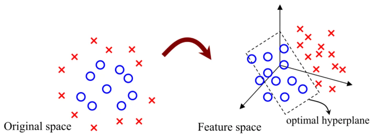
machine (SVM). Unlike traditional methods which minimize the empirical training error, SVM aims at minimizing an upper bound of the generalization error through maximizing the margin between the separating hyperplane and the training data. Hence, it can overcome the poor statistical estimation problem, and it’s relatively higher empirical accuracy and excellent generalization capabilities than other standard supervised classifier (Melgani & Bruzzone, 2004; Fauvel, Chanussot, & Benediktsson, 2006). In particular, SVM have shown a good performance of high dimension data classification with a small size of training samples (Camps-Valls & Bruzzone, 2005; Fauvel, Chanussot, & Benediktsson, 2006) and robustness to Hughes phenomenon (Bruzzone & Persello, 2009; Camps-Valls, Gomez-Chova, Munoz-Mari, Vila-Frances, Calpe-Maravilla, 2006; Melgani & Bruzzone, 2004; Camps-Valls & Bruzzone, 2005; Fauvel, Chanussot, & Benediktsson, 2006). However, there is the most important topic in SVM is kernel method. The main idea of kernel method is to map the input data from the original space to a convenient feature space by a nonlinear mapping where inner products in the feature space can be computed by a kernel function without knowing the nonlinear mapping explicitly and linear relations are sought among the images of the data items in the feature space (Vapnik, 1998; John & Nello, 2004; Schölkopf, Burges, & Smola, 1999). Hence, the most important issue of kernel-based method is ‘‘how to find a proper kernel function’’ for the reference data.
For hyperspectral image classification problems, there is an other problem that the spectral-domain based classifiers often cause the imprecise estimation and have difficulty distinguishing the unlabeled patterns, when the training patterns come from different land-cover classes, but have very similar spectral properties (Jackson & Landgrebe, 2002; Kuo, Chuang, Huang, & Hung, 2009). Figure 1.1 shows the spectral
values obtained from patterns of two categories, Soybeans-min till (purple color) and Corn-no till (yellow color), in the Indian Pine Site dataset. They are two different classes but have very similar spectral properties. Hence, employing some conventional classifiers (e.g. ML classifier, k-nearest neighbor (k -NN) classifier (Fukunaga, 1990), and SVM) by these training patterns would cause the poor classification performance, and the classification maps exhibit a speckle-like classification map (Jackson & Landgrebe, 2002; Kuo, Chuang, Huang, &Hung, 2009). Figure 1.2 shows the classification map of Indian Pine Site which is classified by SVM. There are a number of speckle-like errors on the classification result.
Figure 1.1 These spectral values get from Indian Pine Site dataset. They are two different classes, but have very similar spectral properties. The purple color represents the patterns of Soybeans-min and the yellow color represents the patterns of Corn-notill.
Band
S
Figure 1.2 There are a number of speckle-like errors on the classification result, which is classified by SVM, from the hyperspectral image (Indian Pine Site).
The objectives of this thesis are:
i) To create a proper kernel function for different dataset via a suitable criterion, and compare the performances of some reference kernel functions and composite kernel functions by SVM classifier, and investigate the influences of kernel function.
ii) To develop a spatial-contextual support vector machine (SCSVM) with both spectral information and the spatial contextual information to classify the hyperspectral image, and compare the performances between spectral information based classifiers and spectral and spatial information based classifiers, and investigate the influences of adding the spatial information on the classifiers.
1.2 Organization of Thesis
Chapter 1: A statement of the problem and the purpose of this research are described. Chapter 2: In this chapter, support vector machines (SVM) and Bayesian decision rule
are presented. At SVM aspect, the kernel trick and the multiclass strategies of SVM are introduced. Via the traditional statistical method, Bayesian decision rule, two conventional classifiers, ML classifier and k-NN classifier, are introduced.
Chapter 3: The composite kernel functions are presented via an automatic algorithm. The performances of SVM classifier of different kernel functions explored and reported by the hyperspectral image data and the educational measurement data.
Chapter 4: There are some reference algorithms developed via both spectral and spatial information are introduced, and a novel SCSVM classification algorithm is proposed and introduced to concern both spectral and spatial information for hyperspectral image classification problem, and investigate the mutual effect of spectral and spatial information.
Chapter 5: General conclusions and potentials for future research development are suggested in this chapter.
CHAPTER 2: SUPPORT VECTOR MACHINE AND BAYESIAN
DECISION RULE
In this chapter, some fundamental learning technologies, which are popular in classification issues, are introduced. Section 2.1 focuses on a well-known classification algorithm, support vector machine (SVM) which is a binary classification technique, and the kernel trick and the multiclass strategy are also introduced. In the Section 2.2, the traditional statistical classification technique, Bayesian decision rule, and its extended applications are introduced.
2.1 Support Vector Machine
Support vector machine (SVM) is a popular and promising classification and regression technique proposed by Vapnik and Coworkers (Cortes and Vapnik, 1995; Schölkopf, Burges and Vapnik, 1995; Schölkopf, Burges and Vapnik, 1996; Burges and Schölkopf, 1997). SVM learns a separating hyperplane to maximize margins and produce generalization ability (Burges, 1998). The kernel trick and the multiclass strategy are the most important factor in SVM learning, and hence, they have been introduced by the following paragraphs.
2.1.1 Kernel Trick
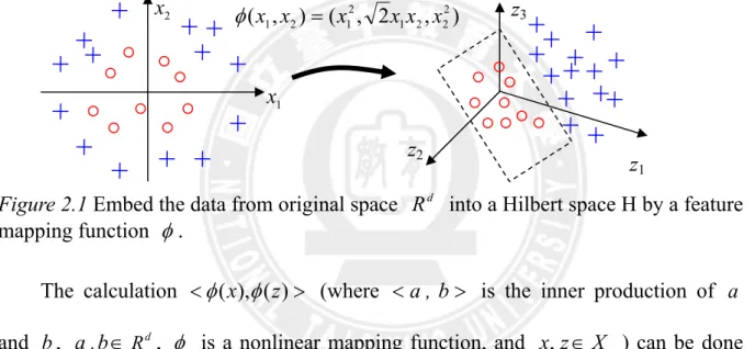
speaking, data with high dimensionality (the number of spectral bands) potentially have better class separability. The strategy of kernel method (John & Nello, 2004) is to embed the data from original space Rd into a feature space H with higher
dimensionality, also call Hilbert space, via a nonlinear mapping function φ ( i.e.,φ:Rd →H), where more effective hyperplanes for classification are expected to exist in this space than in the original space. We illustrate the feature mapping with an explicit function as Figure 2.1.
Figure 2.1 Embed the data from original space Rd into a Hilbert space H by a feature
mapping function φ.
The calculation <φ(x),φ(z)> (where <a , b> is the inner production of a and b , a ,b∈Rd , φ is a nonlinear mapping function, and x,z∈X ) can be done
in input space directly from the original data items via a kernel function, and it is an easier computation. This is based on the fact that any kernel function k:Rd ×Rd →R
satisfying the Mercer’s theorem (John & Nello, 2004), i.e., there is a feature mapping function φ into a Hilbert space H such that
> =< ( ), ( ) ) , (x z x z k φ φ , (2.1)
where x,z∈X , if and only if it is a symmetric function for which the matrices ) , 2 , ( ) , ( 2 2 2 1 2 1 2 1 x x x x x x = φ 1 x 2 x z1 z2 z3
n j i j i z x k ≤ ≤ =[ ( , )]1 , K , (2.2)
formed by restriction to any finite subset {x ,...,1 xn } of the space X are positive semi-definite.
It is worth stressing here that the size of the kernel matrix is N × N and contains in each position K the information of distance among all possible pixel pairs (ij xi
and xj) measured with a suitable kernel function k fulfilling the characterization of kernels and if we use the linear kernel, then the feature mapping φ is an identity map, that is, φ is linear. Otherwise, the feature mapping can be nonlinear. One important idea for using kernel method is without knowing the nonlinear mapping explicitly.
The following are some popular kernel functions.
z Linear kernel: > =< zx z x k( , ) , (2.3) z Polynomial kernel: + ∈ + > < = x z r Z z x k( , ) ( , 1)r, (2.4)
z Gaussian Radial Basis Function kernel (RBF):
} 0 { , 2 exp ) , ( 2 2 − ∈ ⎟ ⎟ ⎠ ⎞ ⎜ ⎜ ⎝ ⎛− − = x z R z x k σ σ (2.5)
2.1.2 Support Vector Learning
Support vector learning is supervised learning algorithm which estimates the entire classification using the principle of statistical risk minimization (Boser, Guyon, & Vapnik, 1992). The basic statistical risk minimization task is to estimate the decision function f :Rd →{ 1± } by a training set from two classes. The training set is
)} ,
{(xi yi with d i ∈R
x ,∀i=1 L, ,n, and yi∈{ 1± } is the class of the pattern x . i
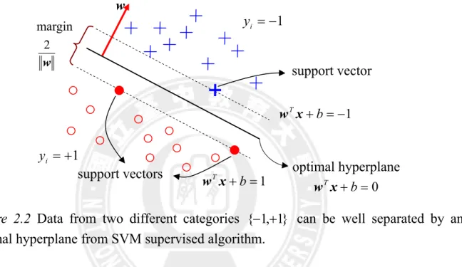
The function f should correctly classify the unlabeled patterns. If these patterns are linear separable, then there exists an optimal vector w and an optimal scalar b such that 1 ) ( + b ≥ y T i i w x , i =1 L, ,n. (2.6)
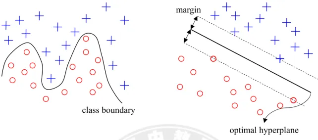
The optimal separating plane (also called optimal hyperplane), wTxi + b=0, should be the one which is the furthest from the closest patterns in these two different classes, and the margin of the separation in Euclidean distance is 2 w . According to the Structural Risk Minimization (RSM), for a fixed empirical misclassification rate, larger margins should lead to better generalization and prevent overfitting in high-dimensional attribute spaces (Bennett & Demiriz, 1998). Hence, we can formulate an optimization problem by maximizing the margin of separation 2 w
and give the constraint functions. This learning algorithm is called a hard-margin support vector machine classifier, because the solutions depend on the patterns (called support vectors), which lie on the margins, wTx+ b=−1 and wTx+ b=1. The
w
maximize 2 w
subject to yi(w⋅xi +b) ≥1, i =1 L, ,n.
(2.7)
The concept of SVM supervised algorithm illustrates as Figure 2.2.
Figure 2.2 Data from two different categories {−1,+1} can be well separated by an optimal hyperplane from SVM supervised algorithm.
Unfortunately, the real data are not always belonged to complete linear separating case. They may mixture and complex, and hence it’s not an easy way to find the
optimal hyperplane directly, such as Figure 2.3. 1 + = i y 1 − = i y optimal hyperplane 0 = + b Tx w support vectors w margin w 2 1 = + b Tx w 1 − = + b Tx w support vector
Figure 2.3 It’s not an easy way to find the optimal hyperplane directly, when data belong to the mixture and complex.
Hence, some training errors (it’s also called empirical risk) (see as Figure 2.4) should be tolerated, and employing the nonlinear feature mapping (see as Figure 2.5) to find the optimal hyperplane of SVM learning in this situation.
Figure 2.4 Enduring some training errors in SVM learning, so these patterns lie between the margins.
margins optimal hyperplane
Figure 2.5 Employing nonlinear feature mapping is easier to find the optimal hyperplane in feature space.
Generally speaking, adding a slack term ξi in SVM learning for each training
pattern to control empirical risk, when some training patterns, which are located on margins, are overlapped, and it’s called soft-margin SVM learning. The soft-margin SVM learning is performed by the following constrained minimization optimal problem: i ξ , minimize w 2 1 1
∑
= + n i i Tw C ξ w subject to i i T i b y(w x + )≥1−ξ , ξi ≥0, ∀i=1 L, ,n (2.8) where ,s iξ are slack variables to control the training errors, and ∈ + 0
R
C is a penalty parameter that permits to tune the generalization capability.
Trying to solve this optimal problem directly with inequality constraints is generally difficult. For this reason, the original constrained optimization problem can be corresponded to an equivalent dual representation by using the Lagrange multipliers (αi ≥0 and βi ≥0) and Lagrange function
∑
∑
= = − + − + − = n i i i n i i i T i i T y b C b L 1 1 ) 1 ) ( ( 2 1 ) , , , (w α β w w α w x ξ βξ . (2.9)This Lagrange function (L(w b, ,α)) has to be minimized with respect to the primal variables ( w , b and ξi) and maximized with respect to the dual variables (αiand
i
β ). According to the Karush-Kuhn and Tucker (KKT) complementarity conditions of the optimization theory, the primal variables must vanish by the derivatives of Lagrange function,
∑
− = ⇒ = ∂ ∂ N i i i i y b L 1 0 ) , , , ( x w w β α w α , (2.10) 0 0 ) , , , ( 1 = ⇒ = ∂ ∂∑
− N i i i y b b L w α β α . (2.11) n i C b L i i i , , 1 , 0 0 ) , , , ( L = ∀ = − − ⇒ = ∂ ∂ α β ξ β α w . (2.12)By substituting (2.10), (2.11) and (2.12) into Lagrange function, the primal optimization problem, which find the primal variables ( w and b ) to minimized the primal objective function, would be replaced by the dual optimization problem, which find the dual variables (αi) to maximized the dual objective function JSVM(α) (2.13). The dual optimization problem has been shown as following:
α maximize
∑
∑∑
− = = − = n i n j j T i j i j i n i i y y J 1 1 1 SVM 2 1 ) (α α αα x x subject to y i C i n n i i i , , 1 , 0 , 0 1 L = ∀ ≤ ≤ =∑
= α α (2.13)The KKT conditions of the constrained minimization optimal problem (2.2) can construct with the optimal solutions (αi),
⎩ ⎨ ⎧ − ⇒ = = + − + i i i i i i T i i y b ξ α ξ β ξ α ) (C 0 0 ) 1 ) ( ( w x . (2.14)
If training patterns are not lay on the margin, then i i T
i b
y (w x + )>1−ξ and αi =0. If the training patterns are lay on the margin, then y ( T i + b)=1
i w x , 0≤αi <C and
0 =
i
ξ . If the training patterns are located between the margins, then
i i
T i b
y(w x + ) =1−ξ , αi =C and ξi ≠0. Hence, optimal scalar b can be obtained by the KKT condition from the support vectors which lie on the margin (see as Figure 2.2), sv n i t T i i i t t t t t T t t n t x x y y b b y , , 1 , 0 , 0 , 0 ) 1 ) ( ( 1 L = ∀ − = ⇒ = > = + − +
∑
= α ξ α ξ α w x (2.15)where xt is the support vector , nsv is the number of support vectors. Once the αi and b are determined, for any new testing pattern xnew
cab be classified by the following decision function,
) sgn( ) ( ~ 1 b y y N i new T i i i new =
∑
+ = x x x α . (2.16)To construct the soft-margin SVM learning of the nonlinear case is computed an optimal hyperplane in feature space via a nonlinear mapping function φ . In other words, constructing soft-margin SVM learning of the nonlinear case is substituted
) (xi
φ for each training pattern xi and separates different classes linearly by the optimal linear separability hyperplane in the feature space. The linear separability hyperplane in the feature space corresponding to the original space is a nonlinear
boundary (see as Figure 2.6).
Figure 2.6 Data from two different categories can be well separated by an optimal hyperplane with an appropriate nonlinear mapping φ which embeds data from the original space (left) to a sufficient higher dimensional feature space (right).
Since all training patterns are mapping to the feature space via nonlinear mapping functionφ , the original dual optimal problem (2.13) could be a more general dual optimal problem as follow:
α maximize
∑∑
∑
∑∑
∑
− = = − = = − = − = n i n j i j i j i j n i i n i n j j T i j i j i n i i k y y y y J 1 1 1 1 1 1 SVM ) , ( 2 1 ) ( ) ( 2 1 ) ( x x x x α α α α φ φ α α α subject to n y i C i n i i i , , 1 , 0 , 0 1 L = ∀ ≤ ≤ =∑
= α α . (2.17)The optimal scalar b obtained by
sv n i i i i t t t t t t T t t n t x x k y y b b y , , 1 , ) , ( 0 , 0 , 0 ) 1 ) ) ( ( ( 1 L = ∀ − = ⇒ = > = + − +
∑
= α ξ α ξ φ α w x (2.18)where xt is the support vector , nsv is the number of support vectors. For any new
optimal hyperplane margin
testing pattern xnew
, the decision function of the more general form is
) ) , ( sgn( ) ) ( ) ( sgn( ) ( 1 1 T b k y b y y n i new i i i n i new i i i new + = + =
∑
∑
= = x x x x x α φ φ α . (2.19) 2.1.3 Multiclass Strategy of SVMSVM attempted to solve a binary two-class problem. The extension from the binary two-class problem to L-classes is an important issue for SVM approach. In this study, we apply two different multiclass strategies, one-against-all and one-against-one, to our experiments, and they are introduced at the following paragraphs.
I. One-against-all multiclass strategy
One-against-all (OAA) multiclass strategy is a ‘‘one class versus all others’’ method (Bottou, Cortes, Denker, Drucker, Jackel, LeCun, et al., 1994). The concept of OAA is constructing L binary decision function if we attempt to solve an L-classes classification problem. When we learn k-th SVM learning, we will see k-th class as positive class ( 1+ ), and the remaining classes will be see as negative class ( 1- ) for all training patterns (see as Figure 2.7).
Suppose we attempt to solve an L-classes problem with a training set )}
,
{(xi yi , d i ∈R
x ,∀i =1 L, ,n , and yi ∈{1,2,L,L}by OAA multiclass strategy SVM. The optimization problem of k-th SVM is formulated by
) ( ) ( , minimizek k ξ w
∑
= + n i k i k T k C 1 ) ( ) ( ) ( 2 1 ξ w w subject to ) ( ) ( ) ( ) ( ( ( ) ) 1 k i k i T k k i b y w φ x + ≥ −ξ , (k) ≥0 i ξ , n i=1 L, , ∀ (2.20) where ⎩ ⎨ ⎧ ≠ − = = k y k y y k i k i k i ( ) ) ( ) ( 1 1 . (2.21)Blue color represents class 1. Green color represents class 2. Purple color represents class 3.
(a) A three class classification problem.
(b) 1-th SVM learning. (c) 2-th SVM learning. (d) 3-th SVM learning. Figure 2.7 A classification example of one-against-all multiclass strategy with three classes. For k-th SVM learning, it should regard k-th class as the positive class, and remaining classes as negative class.
For any new testing pattern xnew, the decision function of SVM with OAA
multiclass strategy is ) ) ( ( max arg ) ( ( )T ( ) , , 1 k new k L k new b y = + = w x x φ L (2.22) y = -1 y = +1 y = +1 y = -1 y = -1 y = +1
where w(k)
and b(k) is the optimal hyperplane and the optimal scalar of k-th SVM
learning, respectively.
II. One-against-one multiclass strategy
One-against-one (OAO) multiclass strategy is ‘‘pairwise classification’’ (Knerr, Personnaz, Dreyfus, 1990). The concept of OAA fits perfectly to the borderline based adaption of SVM. Suppose we attempt to solve an L-classes classification problem. For OAO multiclass strategy, we would construct L(L -1) 2 SVM classifiers, and the k.l-th ( ∀k,l=1,2,L,L. k ≠l ) SVM had been built by k-th class and l-th class, and the remaining classes would be ignored in this step of training learning (show as Figure 2.8).
Suppose we attempt to solve an L-classes problem with a training set )}
,
{(xi yi , d i∈R
x ,∀i=1 L, ,n, and yi ∈{1,2,L,L} by OAO multiclass strategy SVM. The optimization problem of k.l-th SVM is formulated by
) . ( ) . ( , minimizekl kl ξ w
∑
= + n i l k i l k T l k C 1 ) . ( ) . ( ) . ( 2 1 ξ w w subject to ( .)( ( .) ( ) ( .)) 1 (k.l) i l k i T l k l k i b y w φ x + ≥ −ξ , (k.l) ≥0 i ξ ,∀i=1, ,(nk +nl) L , (2.23)where nk is number of training patterns of class k ,nl is number of training patterns
of class l, and ⎩ ⎨ ⎧ = − = = l y k y y kl i l k i k i ( .) ) . ( ) ( 1 1 . (2.24)
testing pattern should be assigned to k-th class, which occurs the maximal number of this pattern assigns to k-th class, according to results of all combination of SVM learning.
Blue color represents class 1. Green color represents class 2. Purple color represents class 3.
(a) A three classes classification problem.
(b) 1.2-th SVM learning by class 1 and class 2.
(c) 1.3-th SVM learning by class 1 and class 3.
(d) 2.3-th SVM learning by class 2 and class 3.
Figure 2.8 A classification example of one-against-one multiclass strategy with three classes. For k.l-th SVM learning, it should regard k-th class as the positive class, l-th class as negative class, and the remaining classes should be ignored in this learning step.
2.2 Bayesian Decision Rule
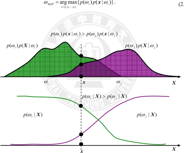
Bayesian decision rule is a statistical learning, and bases on the Bayesian theorem by minimizing the Bayesian error (Fukunaga, 1990). Suppose x is an unknown label pattern. For an L-class {ω1,ω2,K,ωL} classification problem, x can be assigned to one of the L-class which maximizes a posteriori probability (MAP) (Fukunaga, 1990):
)} | ( { max arg } , , 2 , 1 { x i L i MAP p ω ω L = = . (2.25) y = +1 y = -1 y = +1 y = +1 y = -1 y = -1
where p(ωi | x) is the posteriori probability of class ωi, ∀i =1 L, ,L. p(ωi | x) can be calculated by a priori probability p(ωi) and a class-conditional density function p(x|ωi). Figure 2.9 is an illustration of relationship between the posteriori probability and the class-conditional density function. According to the Bayesian theorem, formula (2.25) can be simplified as following:
)} | ( ) ( { max arg } , , 2 , 1 { L i i i MAP p ω p ω ω x L = = . (2.26)
Figure 2.9 An example of Bayes decision rule. The top illustration is the probability distributions of class ωi and ωj, and the below is the posteriori probability of class ωi and ωj. According to MAP, an input sample x will be assigned to class i.
According to the Bayesian decision rule, we can apply different kinds of
x i ω ωj ) | ( ) ( ) | ( ) ( i p i p j p j p ω x ω > ω x ω x ) | ( ) ( j p j p ω X ω ) | ( ) ( i p i p ω X ω ) | ( i X p ω p(ωj |X) ) | ( ) | ( i X p j X p ω > ω X X
class-conditional probability estimation as the class-conditional density function to create different kinds of classifier. The class-conditional density function can be categorized into either parametric or nonparametric probability functions. The well-known parametric classifier, Maximum-likelihood classifier (also called Gaussian classifier), is based on the Gaussian density function (also called normal density function) as the class-conditional density function. Another well-known nonparametric classifier, k nearest neighbor classifier (k-NN), is based on a nonparametric density function as the class-conditional density function. There are two different types of classification classifier, Maximum-likelihood classifier and k-NN classifier, will be introduced in the following sections.
2.2.1 Maximum-likelihood Classifier
Maximum-likelihood classifier (ML) is made up by assuming the samples are following the multivariate normal distribution (Gaussian distribution), with mean vector μi and covariance matrix ∑i of class ω , i ∀i=1 L, ,L . The probability density function of multivariate normal distribution of each class can be represented as follows (Fukunaga, 1990). )} ( ) ( 2 1 exp{ | | ) 2 ( 1 ) | ( 1 2 1 2 i i T i i n i p x − x− μ ∑ x− μ ∑ = − π ω . (2.27)
Hence, the decision rule of ML classifier derives as following (2.28) via MAP estimation (2.26) and formula (2.27).
)} ( ) ( ln ln 2 { min arg 1 } , , 2 , 1 { i i T i i i L i GC MAP = − p + ∑ + x− μ ∑ x− μ − = L ω . (2.28)
2.2.2 k-nearest-neighbor Classifier
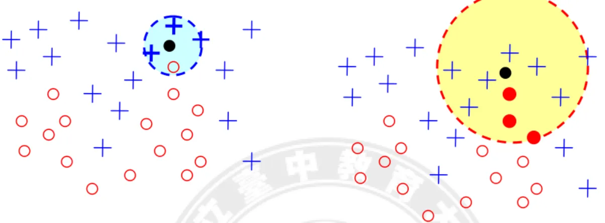
The conception of k-nearest-neighbor classifier (k-NN) is to find the set of k nearest neighbors in the training set to a input sample x, and assign x to the most frequent class among this training set. At the probability viewpoint, k-NN is to extend a local region ν around x until the k-th nearest neighbors is found, and the measure of area in the original space can be seen as one kind of probability density. If the region ν around x is small that means x has a low density. On the contrary, if the density is low, the region ν will grow large and stop until higher density regions are reached (Duda, Hart, & Stork, 2001). We can see the relationship between the local regions of two different classes from the Figure 2.10. The class-conditional probability density estimation of kNN can be represented as (Fukunaga, 1990)
) ( 1 ) | ( x x i i i N k p ν ω = − . (2.29) where n i i n i d n 1/2 1 2 / 1)| | 2 ( Σ Γ π ν = − + . (2.30) and ) ( ) ( ) , (y x = y−x −1 y−x i T i d Σ . (2.31)
where Σ is the distance metric. Therefore, the decision rule of k-NN classifier derives as following (2.32) from MAP estimation (2.26) and the class-conditional probability density estimation of k-NN (2.29).
.} ) , ( ln | | ln 2 1 ln ln { min arg () } , , 2 , 1 { - P N n d i const NN k i i i i L i NN k MAP = − + + + i + = Σ x x ω L . (2.32) where (i) NN ki
x represent k-th nearest neighbor from the training sample i-th class.
Figure 2.10 Examples of the local region around x of 3-NN for two classes. Obviously, the region (left) centering on x to the third nearest neighbors in class i
CHAPTER 3: AN AUTOMATIC ALGORITHM TO CHOOSE
THE PROPER KERNEL
The kernel function plays an important role in the kernel method. For different parameters, the corresponding nonlinear feature mappings and kernel induced feature spaces are different. Hence, how to find a proper kernel function is a crucial issue. In session 3.1, we make an introduction about an automatic algorithm to choose the proper kernel parameter of RBF kernel function. Session 3.2 propose that applying this algorithm to choose a proper composite kernel function.
3.1 Previous Works
Lin, Li, Kuo, and Chu (2010) proposed a novel criterion to choose a proper parameter of RBF kernel function automatically. RBF kernel function (2.5) was introduced from the previous chaapter. According to the formula (2.5), it’s simple to observe that the outcome of RBF kernel function lie in between 0 and 1 obviously. If the Euclidian distance of any two samples approximates to 0, then the outcome of RBF kernel function approximates to 1. In other words, if the Euclidian distance of any two samples is smaller, then the outcome of RBF kernel function is larger, and it represents these two samples are very similar. On the contrary, when the outcome of RBF kernel function is smaller, it means these samples are dissimilar. Hence, how to find a proper parameter makes the outcomes for RBF kernel function from any two samples come
from the same class are closed to 1, and from any two samples come from the different classes are closed to 0 is the very important in the kernel trick.
Suppose i d n i i R i }⊂ , , , { () () 2 ) ( 1 x x
x K is the set of samples in class i , i =1 K,2, ,L.
i
n is the number of the sample from class i. Based on this conception, this algorithm is to find a proper parameter
σ
such thati i r i r n k( (), (), ) 1, , 1,2, , K l l x σ ≈ = x (3.1) and j i n r n k j i j r i , , )≈0, =1,2, , =1,2, , , ≠ ( ( ) ( ) K K l l x σ x . (3.2)
where k(x,y,σ) is a RBF kernel function and (i) l
x is the sample l-th sample from
the i-th class. According to the properties of (3.1) and (3.2), two indices were applied. First is the average of outcomes of RBF kernel function between any two training samples, which come from the same class, and the formula of this conception is denotes as follow:
∑∑∑
∑
= = = = = L i n n r i r i L i i i i σ k n σ W 1 1 1 ) ( ) ( 1 2 ) , , ( 1 ) ( l l x x . (3.3)Second is the average of the outcomes of the RBF kernel function between any two training patterns, which come from different classes, and the formula of this concept is denoted as follow:
∑∑∑∑
∑∑
= ≠ = = = = ≠ = = L i L i j j n n r j r i L i L i j j i j i j σ x x n n σ B 1 1 1 1 ) ( ) ( 1 1 ) , , ( 1 ) ( l l κ . (3.4)It’s simple to observe that 0≤W(σ)≤1 and 0≤ σB( )≤1. However, W(σ) and B(σ) have to close to 1 and 0, respectively. According to the above-mentioned conception, the proper parameter σ can be obtained by minimizing the criterion J(σ).
)} ( ) ( 1 { minimize )} 0 ) ( ( )) ( 1 ( ) ( { minimize 0 0 J σ W σ B σ σ W σ B σ σ> = − + − = > − + . (3.5)
3.2 An Automatic Algorithm to Find a Proper Composite Kernel
The automatic algorithm proposed by Lin, Li, Kuo, and Chu (2010) is to find a proper parameter for RBF kernel. However, the RBF kernel is not always a proper kernel function for all dataset. It may be a more complicated kernel function. According to the closure properties (John & Nello, 2004), we can create more complicated kernel functions from the simple building blocks.
Suppose that κ1,κ2 :X×X →R are the kernel functions, X ⊆Rd , a∈ R+.
The following functions are kernel functions:
) , ( ) , ( ) , (x y κ1 x y κ2 x y κ = + (3.6) ) , ( ) , (x y κ1 x y κ =a (3.7)
follow: ) , ( ) , ( ) , ( ) , (x y 1 1 x y 2 2 x y l l x y composite aκ a κ aκ κ = + +L+ (3.8)
where κi(x,y), i=1 L, ,l, is the basic kernel function, it can be the RBF kernel, polynomial kernel, or any kernel function. ai is the combination coefficient.
From the conception of the reference algorithm, we observe the outcomes of RBF kernel function is closed to 1 or 0, if any pair patterns are similar or dissimilar, respectively. In practice, the outcomes of any kernel functions are not all lie between 0 and 1. Hence, we used the normal kernel to regular the outcomes of basic kernel functions, and the outcome of basic kernel functions would lie between 0 and 1. Normal kernel is defined as follow:
) , ( ) , ( ) , ( ) , ( y y x x y x y x k k k knormal = . (3.9)
In this thesis, two cases will be investigated the effect of combination coefficients. Case 1 is to find the proper combination coefficients without any constraints via the objection function (3.10). Case 2 is to find the proper combination coefficients with some constraint functions, and the constraints are 1
1 =
∑
= l i l a and 0≤{ }
l=1 ≤1 i i a . Thedifferentiation between these two cases is the composite kernel of case 1 is to find a proper kernel for the reference data, and the composite kernel of case 2 is to find the contribution of each basic kernel for the reference data. According to the criterion (3.10) and the kernel function (3.8), we can find the proper combination coefficient set
of case 1 and case 2 by solving the following optimization problem (3.10) and (3.11), respectively:
{
( ) 1 ( ) ( )}
minimize a a a a J = −W +B (3.10) minimize J(a) =1−W(a)+B(a) subject to∑
= = l i 1ai 1, 0≤{ }
=1 ≤1 l i i a (3.11) where∑∑∑
∑
= = = = = L i n n r i r i composite L i i i i k n W 1 1 1 ) ( ) ( 1 2 ) , , ( 1 ) ( l l a x x a (3.12)∑∑∑∑
∑∑
= ≠ = = = = ≠ = = L i L i j j n n r j r i composite L i L i j j i j i j x x n n B 1 1 1 1 ) ( ) ( 1 1 ) , , ( 1 ) ( l l a a κ (3.13) and T l a a , , ] [ 1 L = a .3.3 Experimental Data and Experimental Designs
3.3.1 Hyperspectral Image Data
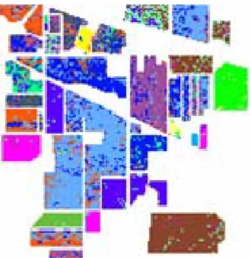
The Indian Pine site (IPS) dataset was gathered by a sensor known as the Airborne Visible/Infrared Imaging Spectrometer (AVIRIS). This dataset was obtained from an aircraft flown at 65000ft. altitude and operated by the NASA/Jet Propulsion Laboratory, with a size of 145×145 pixels and has 220 spectral bands measuring approximately 20m across on the ground. The grayscale IR image and ground truth of IPS are shown in Figure 3.1 and Figure 3.2, respectively. There are 16 different
land-cover classes available in the original ground-truth. Sixteen categories, Alfalfa, Corn-notill, Corn-min, Corn, Hay-windowed, Grass/trees, Grass/pasture-mowed, Grass/pasture, Oats, Soybeans-notill, Soybeans-min, Soybeans-clean, Wheat, Woods, Bldg-Grass-Tree-Drives, Stone-steel towers, would be used in our experiments, and the number of pixels of each class is listed in Table 3.1. In this thesis, IPS hyperspectral image dataset were normalized to the range[0, 1]. In our experiments, we have chosen randomly 10% of the samples for each class from the IPS reference data as training samples, and we take the all samples as the testing set to evaluate the classification performances.
Table 3.1 Sixteen categories and corresponding number of pixels in IPS hyperspectral image.
No. Category #(pixels) No. Category #(pixels)
1 Alfalfa 46 9 Oats 20
2 Corn-no till 1428 10 Soybeans-no till 972 3 Corn-min till 830 11 Soybeans-min till 2455
4 Corn 237 12 Soybeans-clean till 593
5 Hay-windowed 483 13 Wheat 205
6 Grass/trees 730 14 Woods 1265
7 Grass/pasture-mowed 28 15 Bldg-Grass-Tree-Drives 386 8 Grass/pasture 478 16 Stone-steel towers 93
Figure 3.1 A portion of the Indian pine site image with a size of 145×145 pixels. ■ background ■Alfalfa ■Corn-notill ■Corn-min ■Corn ■Hay-windowed ■Grass/trees ■Grass/pasture-mowed ■Grass/pasture ■Oats ■Soybeans-notill ■Soybeans-min ■Soybeans-clean ■Wheat ■Woods ■Bldg-Grass-Tree-Drives ■Stone-steel towers Figure 3.2 The ground truth of Indian pine site dataset.
3.3.2 Educational Measurement Data
The content of the test designed for the sixth grade students is about “Sector” related concepts (see Appendix A). In Figure 3.3, the experts’ structures of the unit for this test are developed by seven elementary school teachers and three researchers. These structures are different from usual concept maps but emphasis on the ordering of nodes. Additionally, every node can be assessed by an item. There are 21 items in this test and 828 subjects are collected in “Sector” tests. According to this structure in “Sector” test, it can divide subjects into six categories of remedial instructions. Table 3.2 is showed the remedial concepts and subjects of each category of remedial instruction.
Figure 3.3 Experts’ structure of “Sector” unit.
Finding the areas of compound sectors
Finding the areas of simple sectors
Definition of sector Finding the areas of circles
Drawing compound graphs
Category Subjects The concepts of remedial instruction
0 80 All concepts are known, they don’t need remedial instructions. 1 50 They are careless and need to practice more.
2 36 “Finding the areas of compound sectors” and “Finding the areas of simple sectors”.
3 47 “Finding the areas of compound sectors” and “Finding the areas of simple sectors”.
4 221 “Definition of sector”, “Finding the areas of compound sectors”, and “Finding the areas of simple sectors”. 5 53
“Drawing sectors”.
“Finding the areas of simple sectors”, “Drawing compound graphs”, and “Definition of sector”.
6 30 “Finding the areas of compound sectors” and “Drawing sectors”.
7 25 “Finding the areas of compound sectors”, “Drawing sectors”, and “Finding the areas of simple sectors”.
8 286 They need to learn all concepts of remedial instruction.
Total 828
For evaluating the performance of the proposed method, twenty subjects in each category are randomly selected to form training datasets, and others are selected to form testing datasets. Table 3.3 is showed the training subjects and testing subjects in the experiment. Category 1 2 3 4 5 6 7 8 Training Subjects 20 20 20 20 20 20 20 20 Testing Subjects 30 16 27 201 33 10 5 266 Total 50 36 47 221 53 30 25 748
Table 3.2 Six categories of remedial instructions.
3.3.3 Experimental Designs
For investigating the performances of these kernel functions, SVM classifier will be the implement to investigate the effective of these kernel functions, and the OAA and OAO multiclass strategies will be applied to the SVM approach. For these two datasets, we will compare the classification performances obtained by i) SVM (OAA and OAO multiclass strategies) with there kernel functions (RBF kernel, polynomial kernel, and composite kernels with constraints and without constraint) ii) ML classifier, and iii) k-NN classifier.
Concerning the SVM classifier, there is a parameter C to control the trade-off between the margin and the size of the slack variables and this experiment adopt the grid search within a given set{0.1,1,10,20,60,100,160,200,1000}. At kernel function aspect, the RBF and polynomial kernel will apply the grid search to our experiments. In both IPS dataset and educational measurement data, the parameter 2σ2 of RBF
kernel will be searched within eleven parts of a range [10−2,10] uniformly,
respectively, and the parameter d of polynomial kernel will be search within a given set d ={1 ,2,3}. For the composite kernel aspect, we create three composite kernels, which apply RBF and polynomial kernel as the basic kernel. First one, named CK1, is the combination of all experimental RBF kernels. Second, named CK2, is the combination of all experimental polynomial kernels. Third, named CK3, is the combination of all experimental RBF kernels and polynomial kernels. There are two approaches, with and without constraints, about this automatic algorithm to search the proper combination coefficients. There are two multiclass strategies, OAA and OAO, apply to SVM. However, the each step of OAO-based SVM is to train the hyperplane of ‘‘i-th class v.s. j-th class (i≠j)’’, and vote any testing sample to either classes, finally
decide this test sample to the class which has the largest vote. That signifies the proper feature space of each step of OAO-base SVM maybe different. Hence, in our experiments we apply this automatic algorithm to find the proper kernel function, named adaptive composite kernel (ACK), for each step of OAO-based SVM.
Concerning the ML classifier, we adopted the Gaussian function as the likelihood function of Bayesian decision rule. Concerning the k-NN classifier, we carried out several trials, varying the value of k from 1 to 20 in order to identify the value that maximizes the accuracy. For simplicity, the model selection for the k-NN classifier was carried out on the basis of the accuracy computed on the testing dataset.
For investigating the performances of all the classifiers, the following measures of classification accuracy would be employed: i) overall classification accuracy (means the percentage of correctly classified samples for all classes), ii) overall kappa coefficient (means the percentage of kappa coefficient calculates for all classes), iii) average accuracy (means the percentage of average of correctly classified samples for each class). Table 3.4 is the framework of experimental designs in this topic.
Dataset Classifier Kernel function
Indian Pine site
Educational Measurement Data
ML k-NN SVM(OAA) SVM(OAO) RBF kernel Polynomial kernel CK1 with constraint CK2 with constraint CK3 with constraint CK1 without constraint CK2 without constraint CK3 without constraint ACK1 with constraint ACK2 with constraint ACK3 with constraint ACK1 without constraint ACK2 without constraint ACK3 without constraint 3.4 Experiment Results and Findings
3.4.1 Hyperspectral Image
According the experiment designs for IPS dataset, we choose 10% of the samples for each class as the training set. However, ML classifier requires estimating the covariance matrices of the classes, the singular problem of covariance matrices and poor estimations would occur, because number of training sample of the class is less than the dimensionality. Therefore, in IPS experiment, the classification results of ML classifier are null. Table 3.5 are shown these validation measures from the best performance of k-NN classifier (k = 1), SVM (OAO and OAA multiclass strategy) with different kernel approaches and the training time about these classification algorithms, and Table 3.6 display the class-specific accuracies from classifiers which
have the highest valid measure. For a convenient reason, we display the classification maps with highest performance from Table 3.5, and these maps shown at Figure 3.3, Figure 3.4, and Figure 3.5, respectively.
Classifier Kernel function
Overall Accuracy (%) Kappa Coefficient (%) Average Accuracy (%) Training time (sec) k-NN 75.5 72.1 74.6 334.4 CK1 with constraint 87.6 85.9 85.8 29972.6 CK2 with constraint 83.3 80.9 80.7 29567.1 CK3 with constraint 87.6 85.9 85.8 23871.2 CK1 without constraint 60.2 54.7 56.6 41381.1 CK2 without constraint 80.4 77.6 78.2 22544.8 CK3 without constraint 86.1 84.1 83.6 15414.6 RBF 87.6 85.9 85.8 336758.1 SVM_OAA Polynomial 83.0 80.6 78.4 240159.7 CK1 with constraint 79.5 77.0 85.1 1769.8 CK2 with constraint 75.9 72.9 81.7 706.9 CK3 with constraint 79.5 77.0 85.3 1903.9 CK1 without constraint 84.8 82.8 85.8 2003.9 CK2 without constraint 72.9 69.9 82.8 872.2 CK3 without constraint 84.8 82.7 85.8 1922.2 ACK1 with constraint 83.8 81.5 80.8 155.5 ACK2 with constraint 74.7 71.8 83.2 49.3 ACK3 with constraint 83.9 81.6 81.9 352.4 ACK1 without constraint 83.2 80.9 80.2 153.6 ACK2 without constraint 77.2 74.5 84.4 47.6 ACK3 without constraint 83.5 81.2 81.5 352.9
RBF 84.0 81.9 85.5 7049.8
SVM_OAO
Polynomial 75.2 72.2 82.0 2231.8
Figure 3.4 The classification map of IPS dataset from k-NN classifier.
(a) CK1 (b) CK2 (c) CK3
SVM (OAA) with constraint
(d) CK1 (e) CK2 (f) CK3
SVM (OAA) without constraint
(g) RBF (h) Polynomial
Figure 3.5 Classification maps of IPS dataset from experimental designs of SVM (OAA).
(a) CK1 (b) CK2 (c) CK3
(d) ACK1 (e) ACK2 (f) ACK3
SVM (OAO) with constraint
(g) CK1 (h) CK2 (i) CK3
(j) ACK1 (k) ACK2 (l) ACK3
SVM (OAO) without constraint
(m) RBF (n) Polynomial
Figure 3.6 Classification maps of IPS dataset from experimental designs of SVM (OAO).
Table 3.6 The percentage of class-specific accuracies from classifiers which have the highest valid measure.
Class SVM_OAA SVM_OAO
No. Number of samples CK1 with constraint CK3 with constraint RBF CK1 without constraint CK3 without constraint 1 46 95.7 95.7 95.7 91.3 91.3 2 1428 85.2 85.2 85.2 81.7 81.7 3 830 75.4 75.4 75.4 77.8 78.0 4 237 84.0 84.0 84.0 89.5 88.2 5 483 92.8 92.8 92.8 91.9 91.9 6 730 95.2 95.2 95.2 96.3 96.3 7 28 75.0 75.0 75.0 96.4 96.4 8 478 97.7 97.7 97.7 94.8 94.8 9 20 60.0 60.0 60.0 60.0 60.0 10 972 86.3 86.3 86.3 86.1 86.0 11 2455 87.0 87.0 87.0 81.5 81.5 12 593 85.8 85.8 85.8 71.8 72.2 13 205 99.5 99.5 99.5 99.5 99.5 14 1265 95.7 95.7 95.7 91.5 91.5 15 386 71.2 71.2 71.2 71.5 71.5 16 93 86.0 86.0 86.0 91.4 91.4
From Table 3.5, Table 3.6, Figure 3.4, Figure 3.5, and Figure 3.6, there are some findings shows as following:
1. SVM can obtain the better performance than k-NN, and the OAA multiclass strategy has the better performance than OAO multiclass strategy. The highest classification performance comes from the SVM (OAA) with CK1 with constraints, CK3 with constraints, and RBF kernel (grid search), and the overall classification accuracy, kappa coefficient, and average accuracy are 87.6%, 85.9%, and 85.8%, respectively. 2. From a formular point of view, composite kernel with constraints is to find the
component of composite kernel approaches to 1 and other components approach to 0, then the algorithm is finding the most important component in composite kernel. 3. In OAA multiclass strategy, the composite kernels (CK1, CK3 with constraints)
applies to SVM can obtain the same result in classification accuracies with RBF (grid search), even in the classification maps. In OAO multiclass strategy, the composite kernel (CK1 without constraint) can gain the better classification performance than RBF and polynomial (grid search). Hence, in OAO, the composite kernel is more suitable than other kernels. However, we can observe that the highest average accuracy of SVM (OAO) is the same with SVM (OAA). In the other hand, SVM (OAO) has the better classification performance in the small size class (i.e. class 3, 4, 7 and 16, see as Table. 3.6).
4. In the training time aspect, the training time of grid search is much greater than composite kernels, no matter what multiclass strategy it is. Hence, applying this automatic algorithm to choose the proper composite kernel can save the training time, and obtain a better or the same classification performance.
3.4.2 Educational Measurement Data
For educational measurement data, Table 3.7 are shown these validation measures from the best performance of ML classifier, k-NN classifier (k = 1), SVM (OAO and OAA multiclass strategy) with different kernel approaches and the training time about these classification algorithms, and Table 3.8 display the class-specific accuracies from classifiers which have the highest valid measure.