風浪生成機制的直接數值模擬

國 立 交 通 大 學

土木工程學系

博 士 論 文

風浪生成機制的直接數值模擬

Direct numerical simulation of wind-wave

generation processes

研究生 : 林媺瑛

指導教授 : 蔡武廷 教授

風浪生成機制的直接數值模擬

Direct numerical simulation of wind-wave generation processes

研 究 生： 林媺瑛 Student : Mei-Ying Lin

指導教授： 蔡武廷 Advisor : Wu-Ting Tsai

國 立 交 通 大 學

土 木 工 程 學 系

博 士 論 文

A Thesis

Submitted to Department of Civil Engineering

College of Engineering

National Chiao Tung University

in Partial Fulfillment of the Requirements

for the Degree of

Doctoral of Philosophy

in

Civil Engineering

April 2007

Hsinchu, Taiwan, Republic of China

風浪生成機制的直接數值模擬

研究生： 林媺瑛 指導教授： 蔡武廷 教授

國立交通大學

土木工程學系博士班

摘 要

利用直接數值模擬的方法，建立一個空氣與水的耦合紊流模式，並以此耦合紊流模 式探討風浪的生成機為本論文的研究重點。其中風浪的生成機制可因風速的不同而不 同，我們僅以低風速下產生的風浪為研究範疇。在考慮低風速的情況下，水面上得到的 平均風應力約為 0.089 dyn cm-2，依此平均風應力而得到的空氣和水的摩擦速度，分別 約為 8.6 cm s-1 _{和 0.3 cm s}-1_{。由於此空氣與水的耦合紊流模式，在空氣與水的介面上，} 同時滿足速度與應力連續的條件，所以這個耦合模式可以同時捕捉到空氣與水體的運動 和它們之間的交互作用。研究顯示，發展最快之波浪的波長與實驗的量測結果很接近， 波長約為 8~12 公分。而且，在波浪生成之後，因波浪成長速率的不同，可分為線性與 指數成長兩階段，也與理論和觀測的結果相同。但是，受限於在空氣與水的介面處使用 了線性的邊界條件，因此當波浪的梯度大於 0.01 時，即無法再利用此耦合模式繼續進行 模擬。模擬的時間間隔，約為波浪開始生成之後 70 秒內的發展過程。波浪生成之後， 我們分析了波浪對空氣與水體中紊流場的影響；也執行了一些敏感性測試，包括水體中 的紊流場、表面張力和空氣的高度。藉由與理論的結果比較，在線性的成長階段，我們 的波浪成長率只有在較高的空氣高度的算例中，與 Phillips (1957) 的理論預測較一致； 在指數的成長階段，有些的波浪成長率與 Belcher & Hunt (1993)的理論預測、Plant (1982) 所統計的實驗觀測和一些數值模擬的結果一致。但是，有些波浪的成長率則較前人的研 究結果大 2~3 倍。雖然在量的比較上與前人的結果有些許的差異，但是在風浪生成機制 的定性條件上，和 Phillips (1957)與 Belcher & Hunt (1993)所提的機制是符合的。風的能

量能夠傳輸至波浪的主要因素：在線性的波浪成長階段，如 Phillips (1957)所提的機制一 樣，來自紊流所引起的壓力擾動；在指數的波浪成長階段，如 Belcher & Hunt (1993)所 提的機制一樣，來自波浪所引起的壓力擾動與波浪之間所形成的形狀阻力。

Direct numerical simulation of wind-wave generation processes

Student : Mei-Ying Lin Advisor : Professor Wu-Ting Tsai

Department of Civil Engineering

National Chiao Tung University

ABSTRACT

An air-water coupled model is developed to investigate wind-wave generation

processes at low wind speed where the surface wind stress is about 0.089dyncm-2 and the

associated surface friction velocities of the air and the water are u∗_a ~8.6cms-1 and -1 s cm 3 . 0 ~ ∗ w

u , respectively. The air-water coupled model satisfies continuity of velocity and stress at the interface simultaneously, and hence can capture the interaction between air and

water motions. Our simulations show that the wavelength of the fastest growing waves agrees

with laboratory measurements

(

λ ~8−12cm

)

and the wave growth consists of linear and exponential growth stages as suggested by theoretical and experimental studies. Constrained

by the linearization of the interfacial boundary conditions, we perform simulations only for a

short time period, about 70s; the maximum wave slope of our simulated waves is ak ~0.01 and the associated wave age is c u_a∗ ~5, which is a slow moving wave. The effects of waves on turbulence statistics above and below the interface are examined. Sensitivity tests are

carried out to investigate the effects of turbulence in the water, surface tension, and the

numerical depth of the air domain. The growth rates of the simulated waves are compared to

Phillips’ (1957) theory for linear growth and to Plant’s (1982) experimental data and previous

simulation results for exponential growth. In the exponential growth stage, some of the

simulated wave growth rates are comparable to previous studies, but some are about 2~3

times larger than previous studies. In the linear growth stage, the simulated wave growth rates

prediction only for the larger air domain. In qualitative agreement with the theories proposed

by Phillips (1957) and Belcher and Hunt (1993) for slow moving waves, the mechanisms for

the energy transfer from wind to waves in our simulations are mainly from

turbulence-induced pressure fluctuations in the linear growth stage and due to the in-phase

relationship between wave slope and wave-induced pressure fluctuations in the exponential

ACKNOWLEDGEMENTS

I would like to express my sincere gratitude to Wu-Ting Tsai on the development of

air-water coupled model and Chin-Hoh Moeng on the study of wind-wave generation

processes and English writing for their truly excellent guidance and support during the past

few years. Their outstanding ability for research and providing good education for student

help me to achieve more than I ever thought possible. With their discreet and careful guard

contributes to the accomplishment of this work. I would like to thank Wu-Ting again for the

chance he gave me to study with Chin-Hoh at NCAR in U.S.A for one and half year. During

that period, discussing some scientific questions with other scientists or attending a lot of

seminars helped me to learn more about scientific work and induced the enthusiasm for

research inside me. A special thanks goes to Peter Sullivan for his useful comments and

suggestions about the wind-wave generation processes on this work. Peter also provided some

data of measurements and simulation results as shown in figure 20 of this thesis. Thanks to

Stephen Belcher who provides some comments on theoretical studies of wind-wave

generation processes. I would also like to thank the members of my committee, Ching-Yuang

Huang, Keh-Chia Yeh, Wu-Shung Fu, Wen-Yih Sun, for their comments and suggestions on

my work.

Thanks to Wu-Ting’s research group. Those experiences we shared together become

good memories in my mind. A special thanks to Shi-Ming Chen for helping me to deal with

my computer.

Thanks to my friends for bringing me a lot of joy and enriching my life.

This work was mainly supported by grants from the National Science Council of Taiwan

under contract numbers NSC 90-2611-M-009-001 and 91-2611-M-008-002, and a part of this

study was sponsored by the National Science Foundation through the National Center for

TABLE OF CONTENTS

Chinese abstract……….iii Abstract………v Acknowledgements………vii Table of contents…..……….……….ix List of tables………..xi List of figures………..xii List of symbols………..xviii

I. Introduction………...1

II. The coupled model……….3

1. Flow Configuration………..3

2. Governing Equations………4

3. Boundary Conditions………...5

4. Numerical Method………...7

5. Initialization……….8

III. Flow visualization………..14

1. Waves and streaks………..14

2. Pressure and stress fields………15

IV. Characteristics of the surface waves……….24

V.

Wave effect on flow fields………..28

1. Wave effect on mean velocity profiles………...28

2. Wave effect on turbulence intensities………...29

VII. Comparing with wind-wave generation mechanisms……….37

1. Linear growth stage………37

2. Exponential growth stage………...39

VIII. Sensitivity tests………..43

1. The effects of turbulence in the water……….43

2. The effects of surface tension………..44

3. The effects of the computational domain of air………...44

IX. Conclusions……….46

Appendixes ………48

A. Numerical Method………48

I. Pressure Poisson equations………..48

II. Stretching grid systems………48

B. Initialization………..49

I. Analytical solution: the mean velocity profile of the coupled air-water flow…….49

II. Generating turbulence by Buoyancy force……….51

C. Decomposition of the flow field in the Water……….53

D. Some records for four simulation runs………...60

E. Future Work………..…76

References………...77

LIST OF TABLES

Table 1: Dominate waves and the percentage of each wave energy at early (t~15s) and late

(t~68 s) stages for the control case. Note that the dominate waves at these two

stages are different………27

Table 2 Dominate waves and the percentage of each wave energy at early (t~15s) and late

(t~68 s) stages for the simulation without generating turbulence in the water at the

beginning of the simulation. ……….73

Table 3 Dominate waves and the percentage of each wave energy at early (t~15s) and late

(t~68 s) stages for the simulation without surface tension effect. ………..74

Table 4 Dominate waves and the percentage of each wave energy at early (t~15s) and late

LIST OF FIGURES

Figure 1: Numerical domain of two immiscible turbulent flows driven by velocity U on a ₀ Cartesian coordinate. The interface of air and water is located at z=0. The size of air and water sub-domains is the same,

(

L_x ,L_y ,h

)

=

(

6 ,6 ,1

)

h. ………10

Figure 2: Location of velocity components and pressure on staggered grid systems for the

mixed finite-differencing and pseudospectral scheme. Symbols with solid circle and

cross are ghost points at the interface. ……….11

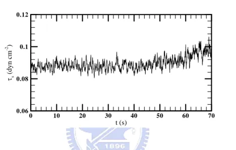
Figure 3: Time evolution of the mean wind stress τ_s at the interface. ………..12

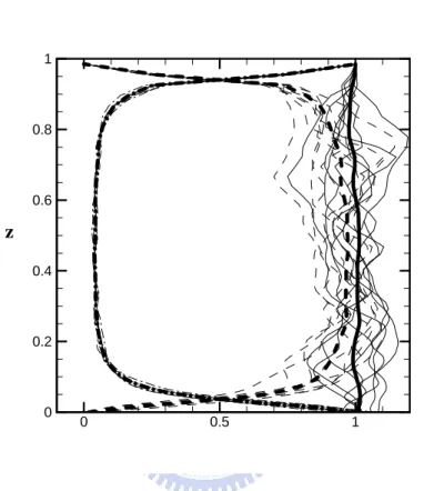
Figure 4: Vertical profiles of dimensionless mean vertical turbulent flux − u ′_a′w_a

( )

u*_a 2(thick dashed line), viscous flux

(

ν_a u_a*h

)

∂U_a ∂z (thick dash-dotted line), and their sum (thick solid line) in the air. The thin lines represent these terms at various time

instances during 50 to 70 s, while the thick lines are their averages. ……… 13

Figure 5: Snapshots of the instantaneous surface wave height η (left panels) and streamwise velocity u at the interface (right panels) at time t =2.6s, 16s and 64s (from top to bottom), respectively. ……….17

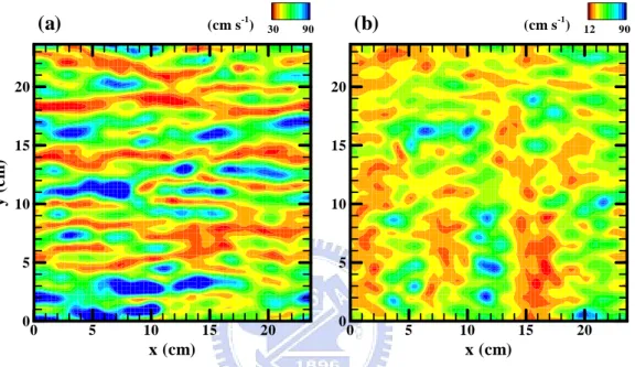
Figure 6: Snapshots of the instantaneous streamwise velocity u within the viscous sublayer _a of the air domain at time t=2.6s (a) and 64s (b). ………...18

Figure 7: Representative iso-surfaces of vertical velocity in the water at time t=2.6s (a) and t =66s (b). Black and grey iso-surfaces show vertical velocity for values

-1 s cm 5 . 1 − and 1.5cms-1, respectively. ………19

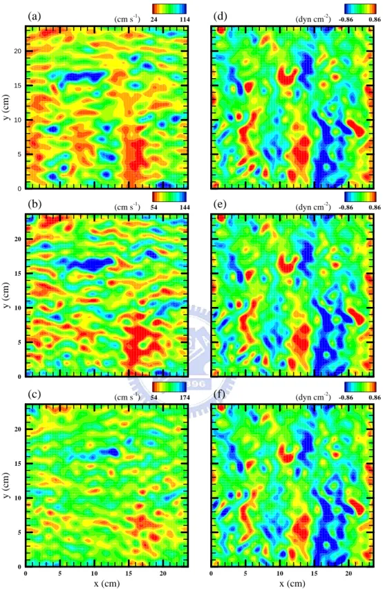
Figure 8: Snapshots of the instantaneous streamwise velocity (left panels) and pressure

fluctuations (right panels) of the air flow in

( )

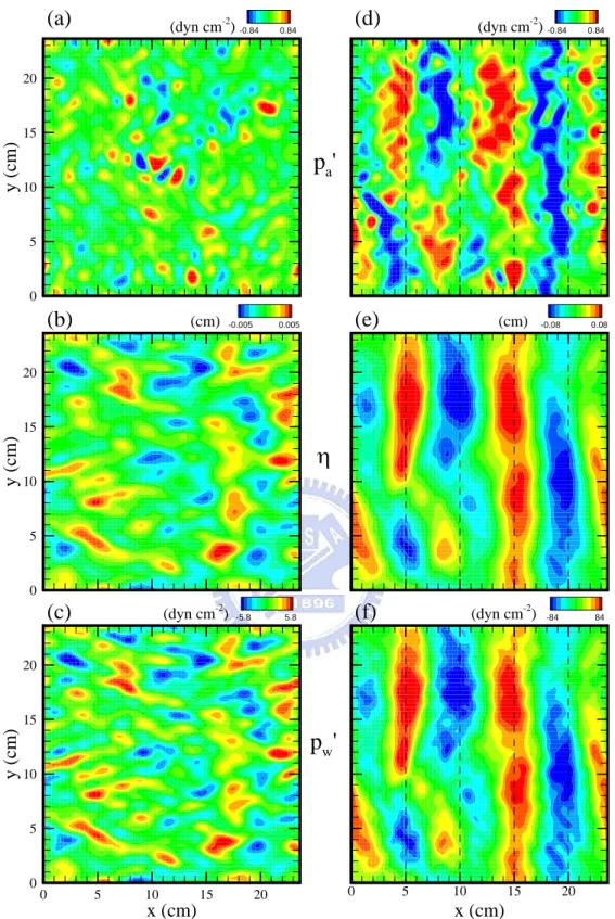
x,y −planes at t=64s at three different heights. The upper panels are within the viscous sublayer z=0.045cm, middle panels are in the matched layer z=0.23cm, and lower panels are in the inertial sublayer z=0.37cm. ……….20

Figure 9: Snapshots of the instantaneous pressure fluctuations in the air p′ (a, d) and water _a w

p′ (c, f), and wave height η (b, e) on the interface at time t=16s (left column) and t =66s (right column). ………...21

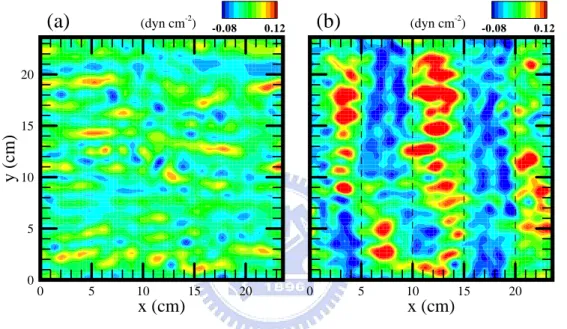
Figure 10: Snapshots of the instantaneous shear stress fluctuations τ_s′ at the interface at time s

16 =

t (a) and t=66s (b). ……….22

Figure 11: Snapshots of instantaneous pressure fluctuations in the air p′ and water _a p′ in _w an

( )

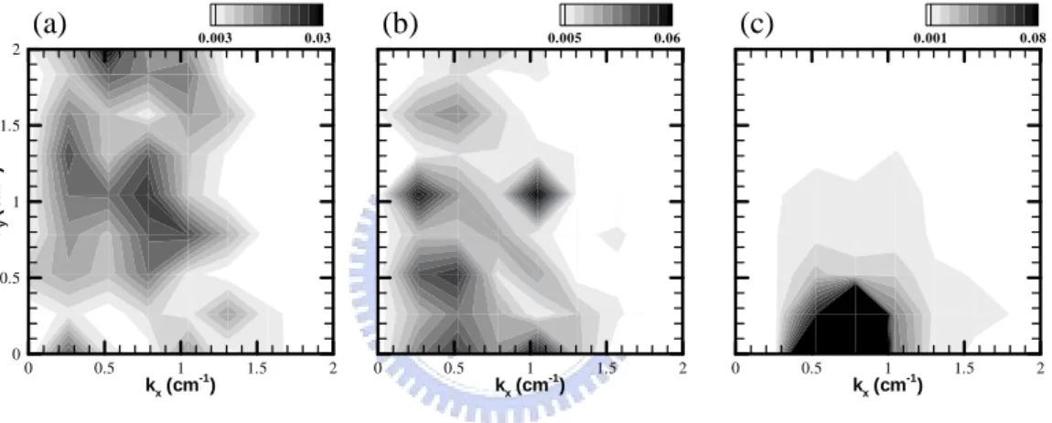
x,z −plane and the associated surface wave height η at time t=16s (figures a-c) and t =66s (figures d-f). The cross section is located at y=7.5cm in figure 9. η is normalized by its maximum value at this time. ………..23

Figure 12: Wavenumber spectra of surface wave height ηˆ

(

k ,_x k_y

)

(normalized by its total energy) at time t=0.5s (a), t=16s (b) and t=64s (c). Note that the maximum contour level in (c) is higher than that in (a) and (b). ……….25

Figure 13: Wavenumber-frequency spectrum of the surface wave height ηˆ

(

k_x,σ

)

(normalized by its total energy) at time interval t=66~66.5s for k_y =0. The dashed line represents the linear dispersion relation σ k_x =U_s + g k_x where

12 = s

U cm s-1 is the mean surface current. ………26

and delta symbols denote the matched linear-logarithmic profiles at t =16s and s

70 =

t , respectively. The log-law constants used to collapse the profiles

( )

κ, z0+ are (0.34, 0.31) and (0.33, 0.84) in the air and

( )

κ, z₀+ are (0.3, 1.55) and (0.37, 0.3) in the water at time t =16s and t=70s, respectively. ………30

Figure 15: Vertical distributions of the normalized turbulent velocity variances of the air

(upper panels) and of the water (lower panels) at early (t=16s) and later (t=64s) stages. ………..31

Figure 16: Time evolution of interfacial parameters: (a) root-mean-square of the surface wave

height 〈η2〉12, (b) root-mean-square of pressure fluctuations 〈p′_a2〉12, (c) form stress D , (d) mean surface current _p U , (e) root-mean-square of shear stress _s fluctuations 〈τ′_s2〉12 and (f) surface roughness length z of the air. …………...34 ₀+

Figure 17: Time evolutions of wave amplitudes of the five fastest growth waves at early stage

(a), and the three fastest growth waves at late stage (b). Note that we use a linear

coordinate for (a) but an exponential coordinate for (b). ……….35

Figure 18: Time evolution of the form stress D for the same wave modes as those shown in _p figure 17. ………..36

Figure 19: The comparison of the mean square surface wave height between our numerical

results 〈η2〉 (solid lines) from four simulations and the theoretical predictions 〉

〈ξ2

(dashed-dotted lines) of Phillips (1957). The four simulations are : (a) the

control run with the height of the air domain h = 4 cm, (b) the run with no initial

turbulence in the water, (c) the run with no surface tension and (d) the run with the

height of the air domain h = 8 cm. For the theoretical curves, U_c =18u_a* is used. ………...41

Figure 20: Wave growth rate as a function of inverse wave age. Small symbols are results

from the measurements (synthesized by Plant, 1982) and the simulation results (Li,

1995; Sullivan & McWilliams, 2002) as published in Sullivan & McWilliams

(2002). The dashed lines are the empirical formula β =

(

0.04±0.02

)(

u* c

)

2 proposed by Plant (1982) The cross and large triangle symbols are our results

calculated from the growth of wave amplitude (7.3) and from the form stress (7.4),

respectively, for the three fast-growing wave components. The three fast-growing

wave components are

(

k_x,k_y

)

=

(

0.78,0.

)

,

(

0.52 ,0.

)

and

(

0.78 ,0.26

)

cm for the -1 control simulation (a),

(

0.52 ,0.

)

,

(

0.78 ,0.26

)

and

(

0.52,0.26

)

cm for the -1 simulation with no initial turbulence in the water (b),

(

0.78 ,0.

)

,

(

0.52,0.26

)

and

(

0.52,0.

)

cm for the simulation with no surface tension (c), and -1

(

0.52,0.

)

,

(

0.78,0.

)

and

(

0.78,0.26

)

cm for the simulation with larger air domain (d). -1 ………..42

Figure 21: Wavenumber spectra of surface wave height ηˆ

(

k ,_x k_y

)

(normalized by its total energy) at time t=16s (left panels) and t=64s (right panels) for the control case shown in (a, b), the simulation without generating turbulence in the water at

the beginning of the simulation shown in (c, d), the simulation without surface

tension at the interface in (e, f), and the simulation doubling the height of the

computational domain of the air in (g, h). ………45

Figure 22. The decomposition of surface wave height near time t~65 s. With the application of

decomposition method in Appendix C, the total surface wave height (a, b) can split

into wave-correlated components (c, d) and wave-uncorrelated components (e, f).

The difference between left and right columns is the cutoff frequency (or

wavenumber). The cutoff frequency (wavenumber) of left column is smaller (larger)

Figure 23. As figure 22 but for the decomposition of streamwise velocity at the interface.

……….57

Figure 24. As figure 22 but for the decomposition of spanwise velocity at the interface. …..58

Figure 25. As figure 22 but for the decomposition of vertical velocity at the interface. …….59

Figure 26. As figure 3 but for (a) the control run with the height of the air domain h = 4 cm, (b) the run with no initial turbulence in the water, (c) the run with no surface tension

and (d) the run with the height of the air domain h = 8 cm. ………..62

Figure 27. As figure 4 but for (a) the control run with the height of the air domain h = 4 cm, (b)

the run with no initial turbulence in the water, (c) the run with no surface tension

and (d) the run with the height of the air domain h = 8 cm. ………..63

Figure 28. As figure 5 but for the run with no initial turbulence in the water. ………64

Figure 29. As figure 5 but for the simulation without surface tension at the interface. ……..65

Figure 30. As figure 5 but for the simulation doubling the height of the computational domain

of the air. ………66

Figure 31. Wavenumber spectra of surface pressure fluctuations of the air (normalized by its

total energy) at time t=16s (left panels) and t=64s (right panels) for the control case shown in (a, b), the simulation without generating turbulence in the

water at the beginning of the simulation shown in (c, d), the simulation without

surface tension at the interface in (e, f), and the simulation doubling the height of

Figure 32. As figure 16 but for the run with no initial turbulence in the water. ………..68

Figure 33. As figure 16 but for the simulation without surface tension at the interface. …….69

Figure 34. As figure 16 but for the simulation doubling the height of the computational

domain of the air. ………..70

Figure 35. As figure 17 but for the control case shown in (a, b), the simulation without generating turbulence in the water at the beginning of the simulation shown in (c,

d), the simulation without surface tension at the interface in (e, f), and the

simulation doubling the height of the computational domain of the air in (g, h).

………71

Figure 36. As figure 18 but for the control case shown in (a, b), the simulation without

generating turbulence in the water at the beginning of the simulation shown in (c,

d), the simulation without surface tension at the interface in (e, f), and the

simulation doubling the height of the computational domain of the air in (g, h).

LIST OF SYMBOLS

a Wave amplitude L

b A constant related to surface roughness length -

c Phase velocity L T-1

E Wave energy density M T-2

p

D Form stress; Form drag M L-1 T-2

g Gravitational acceleration LT-2

h Height L

l

H The divergence of the convective and diffusive terms M L-3 T-2

k Wavenumber k = k_x2 +k_y2 L-1 y x k k , _{Wavenumber components L}-1 y x L

L , Horizontal length components L-1

z y

x N N

N , , _{Grid point components -}

p Pressure M L-1 T-2

a

p Pressure of the air M L-1 T-2

a

p′ Pressure fluctuations of the air M L-1 T-2

w

p Pressure of the water M L-1 T-2

w

p′ Pressure fluctuations of the water M L-1 T-2

a

Re Reynolds number of the air -

w

Re Reynolds number of the water -

∗ a

Re Wall Reynolds number of the air -

∗ w

Re Wall Reynolds number of the water -

t Time T

u,v,w Cartesian velocity components L T-1

a a

a v w

u , , Cartesian velocity components of the air L T-1 w

w

w v w

u , , Cartesian velocity components of the water L T-1 a

a

a v w

w w

w v w

u′, ′, ′ Cartesian velocity fluctuations components of the water L T-1 ∗

a

u Friction velocity of the air L T-1

∗ w

u Friction velocity of the water L T-1

a

U Mean velocity of the air L T-1

w

U Mean velocity of the water L T-1

s

U Mean current at the interface L T-1

o

U Constant velocity imposed at upper boundary L T-1 c

U Convection speed of pressure fluctuations L T-1

+

U Non-dimensional wall velocity -

x,y,z Cartesian coordinates L

+

z Non-dimensional wall coordinate -

+ 0 z Surface roughness - z y x Δ Δ

Δ , , Grid size components L

+ + _Δ

Δx ,_a y_a Horizontal grid size of the air in wall units - +

+ _Δ

Δx ,_w y_w Horizontal grid size of the water in wall units -

l

α Coefficient of thermal expansion oK-1

β Dimensionless wave growth rate -

∗

β Wave growth rate T-1

ε

Dissipation rate L2 T-3

γ _{Surface tension M T}-2

η _{Surface wave height L}

κ Von Karman constant -

λ

Wavelength L

a

μ Dynamic viscosity of the air M L-1 T-1

w

μ Dynamic viscosity of the water M L-1 T-1

a

ν Kinematic viscosity of the air L2 T-1

w

ν Kinematic viscosity of the water L2 T-1

a

w

ρ Density of the water M L-3

σ _{Wave radian frequency T}-1

τ Surface shear stress M L-1 T-2

τ′ Surface shear stress fluctuations M L-1 T-2

s

τ Mean surface shear stress M L-1 T-2

υ _{Root-mean-square fluctuating speed L T}-1

ξ Theoretical prediction of surface wave height L

ζ Kolmogorov microscale L

Κ Thermal diffusivity L2T-1

o a

θ Reference temperature of the air oK

o w

θ Reference temperature of the water oK

a

θ Temperature of the air oK

w

θ Temperature of the water oK

a

h Thermal conductivity of the air JT-1L-1oK-1

w

h Thermal conductivity of the water JT-1L-1oK-1

a p

C Heat capacity of the air JM-1oK-1

w p

Chapter I

Introduction

As wind flows over a water surface, air and water motions interact and induce many

phenomena at the interface. Wind-generated waves are the most visible signature of this

interaction and play a major influence on the momentum and energy transfer across the

interface. These wind-generated waves, observed by microwave-radar backscatter, have

wavelengths of the order of 4-40 cm (Massel, 1996). Because these small-scale waves impact

remote sensing of the sea surface, the generation and growth of wind-generated waves have

been subjects of intense research. However, the mechanisms that generate these surface waves

are still an open issue due to (1) difficulties in obtaining a dataset from laboratory and field

measurements that records the time evolution of motions in both atmosphere and ocean

domains, (2) mathematical difficulties in dealing with highly turbulent flows over complex

moving surfaces, and (3) lack of a suitable coupled model to simulate turbulent flows in both

atmosphere and ocean simultaneously. With increases in computer power, it is now possible to

simulate wave and turbulence phenomenon by direct numerical simulation (DNS). DNS

numerically solves the Navier-Stokes equation subject to boundary conditions and hence such

simulated flow fields contain no uncertainties other than numerical errors. In this study we

develop an air-water coupled DNS model and use it to study wind-wave generation and

growth processes.

Theoretical studies (Jeffreys 1925; Phillips 1957; Phillips & Katz 1961; Miles 1957;

Townsend 1972, 1980; Phillips 1977; Jacobs 1987; Kahma & Donelan 1988; van Duin &

Janssen 1992 and Belcher & Hunt 1993, among many others) have proposed different

mechanisms as to how surface waves are generated from calm water and quantify the

exponential growth regimes for surface waves.

With the increase of computer power, the numerical simulation (DNS) technique has

become a useful tool in studying turbulent flows. Such a numerical simulation, by directly

solving the fluid dynamics equations, produces three-dimensional, time evolving flow fields

which can be analyzed to study the details of the flow structure and to deduce the turbulence

statistics. However, most of the previous numerical studies (Davis 1970; Gent & Taylor 1976;

Al-Zanaidi & Hui 1984; De Angelis et al. 1997; Henn & Sykes 1999; Sullivan et al. 2000;

Tsai et al. 2005) examine either the wave effect on air motions or the wind stress effect on

water motions by simulating only air or water flows (i.e., one-phase flow). These so-called

one-phase flow simulations are driven by either wind shear near the surface for turbulence in

the air or an imposed surface stress for turbulence in the water. Because the interface is

prescribed, the interaction between the wind and the waves is prohibited. Only a few

numerical studies are conducted for two-phase flows (Lombardi et al. 1996; De Angelis 1998;

Fulgosi et al. 2003) but none of them investigate the wind-wave generation processes. The

present study, therefore, is aimed at unraveling wind-wave generation processes by

conducting direct numerical simulations that couple turbulent air and water flows.

The organization of this paper is as follows. The numerical aspects of the present

simulation, including the model formulation, numerical method and simulation

implementation are described in section 2. The simulated flow structures of surface waves and

elongated streaks generated by wind are shown in section 3. The wave effect on the statistics

of mean velocity and turbulent intensity is reported in section 4. The characteristics of the

generated surface waves are examined in section 5. Two wave growth types are defined in

section 6. Comparison with theoretical wind-wave generation mechanisms is given in section

7. The effects of turbulence in the water, surface tension, and the numerical domain in the air

side on wave growth are examined in section 8. Finally, the main conclusions of this paper are

Chapter II

The coupled model

II.1 Flow configuration

Consider two turbulent flows, air and water, under a wind-driven system that interacts

across a deformable interface. The turbulent and wave motions must satisfy the continuity of

velocity and stress across the interface. As a first step, we simplify the problem by excluding

the non-linearity of waves and wave breaking effect and linearized these interfacial boundary

conditions via the small amplitude wave assumption. We use the coupled model to study the

initial stage of the generation of waves by wind.

First we have to choose the characteristic velocity and length scales of the flow. In the

study of a turbulent flow over given water waves, Sullivan et al. (2000) chose the constant

velocity imposed at the upper boundary and the wavelength of the imposed water wave as the

characteristic scales. In the study of turbulent shear flow under a free surface, Tsai et al. (2005)

used the mean velocity at the free surface and the length of viscous sub-layer given from

experimental result (Melville et al., 1998) as their characteristic scales. Flow features are

typically characterized by their external condition: a given wave or imposed wind speed,

which make it easy to choose the characteristic scales, such as above studies of single-phase

turbulent flows. For two-phase flows we investigate here, there are two problems in choosing

the characteristic scales. First is due to the deformable interface that is not a fixed wave type.

The interface changes with time and varies from place to place. This boundary does not

provide any characteristic length for us to define the domain size or the bulk Reynolds

due to the different time and length scales of turbulent motions in air and water. In general, we

should use two sets of characteristic variables to measure these two motions. But U is the 0 only characteristic flow feature we know before starting the simulation.

Thus, we consider two turbulent flows (air and water) interacting across a deformable

interface under a wind-driven system. Each domain of the two immiscible fluids is a

rectangular box with a depth h and horizontal length (L_x,L_y)=6h, as shown in figure 1. We adopt a Cartesian coordinate where the air region occupies the z≥0 domain, and the water region the z≤0 domain. The horizontal coordinates x and y are in the streamwise and spanwise directions, respectively. The external forcing of the system is a constant velocity

0

U imposed at the upper boundary (z=h) in the air region, i.e., similar to a Couette flow. We set U₀ =3ms-1 in this study.

II.2 Governing equations

The mass and momentum conservation equations for incompressible, Newtonian

fluids of air and water with density ρ_l and kinematic viscosity ν_l are 0 = ⋅ ∇ u_l , (2.1) l l l l l l l _{u u u} u + ⋅∇ =− 1 ∇ + ∇2 ∂ ∂ _ν ρ p t , (2.2)

where the subscript _l denotes variables in air (_l=a) or water (_l=w), u=

(

u ,,v w

)

are velocity components in streamwise, spanwise and vertical directions respectively, and p is _l the pressure.

The Poisson equation for p is obtained by taking the divergence of (2.2) and using _l (2.1) l l l l _Η z p y p x p = ∂ ∂ + ∂ ∂ + ∂ ∂ 2 2 2 2 2 2 , (2.3)

equation (2.2). The solution of (2.3) forces the continuity equation (2.1) to be satisfied at each

time step.

II.3 Boundary conditions

The domains of the two immiscible fluids have six external boundaries and one

internal deformable interface. For external boundaries, periodic conditions are assumed on the

four sidewalls of the computational domain. At the top of the domain, z=h , a constant-velocity condition is applied as

0 U u_a = , 0v_a = , wa =0, _∂ =0 ∂ z p_a . (2.4)

At the lower bottom of the water region, z=−h, we impose free-slip boundary conditions 0 = ∂ ∂ z u_w , =0 ∂ ∂ z v_w , 0w_w = , =0 ∂ ∂ z p_w , (2.5)

to emulate an infinite depth.

For the deformable boundary, the interface of two viscous fluids must satisfy the

following requirements as stated in Wehausen & Laitone (1960):

1. The effect of surface tension as one passes through the interface is to produce a discontinuity in the normal stress proportional to the mean curvature of the boundary surface. 2. For viscous fluids the tangential stress must be continuous as one passes through the interface.

3. For viscous fluids the tangential component of the velocity must be continuous as one passes through the interface.

Without simplification, these requirements lead to complicated boundary conditions (see

equations 3.2~3.6 in Wehausen & Laitone, 1960). However, assuming small interfacial

deformation, as in the initial wind-wave generation processes considered here, we can

satisfied at z=0 as follows: u_a =u_w, v_a =v_w, w_a =w_w, (2.6) ⎟ ⎠ ⎞ ⎜ ⎝ ⎛ ∂ ∂ + ∂ ∂ = ⎟ ⎠ ⎞ ⎜ ⎝ ⎛ ∂ ∂ + ∂ ∂ x w z u x w z u _{w w} w a a a μ μ , (2.7) _⎟⎟ ⎠ ⎞ ⎜⎜ ⎝ ⎛ ∂ ∂ + ∂ ∂ = ⎟⎟ ⎠ ⎞ ⎜⎜ ⎝ ⎛ ∂ ∂ + ∂ ∂ y w z v y w z v _{w w} w a a a μ μ , (2.8) ⎟⎟ ⎠ ⎞ ⎜⎜ ⎝ ⎛ ∂ ∂ + ∂ ∂ − = ⎟⎟ ⎠ ⎞ ⎜⎜ ⎝ ⎛ ∂ ∂ + ∂ ∂ − + − ⎟⎟ ⎠ ⎞ ⎜⎜ ⎝ ⎛ ∂ ∂ + ∂ ∂ + − 2 2 2 2 2 2 y x y v x u g p y v x u g p a a a a a w w w w w η η γ μ η ρ μ η ρ , (2.9)

where μ_a ≡ρ_aν_a and μ_w ≡ρ_wν_w are dynamic viscosities of air and water, and γ is the surface tension of the water interface. The linearized kinematical condition satisfied at z = 0 is

w y v x u t ∂ = ∂ + ∂ ∂ + ∂ ∂η ( η) ( η) . (2.10)

The use of a central-differencing scheme at the interface requires additional points

(ghost points) below the interface for

(

u_a,v_a,w_a,p_a

)

and above the interface for

(

uw,vw,ww,pw

)

, as shown in figure 2. The

(

ua,va,uw,vw

)

values at the ghost points are determined using the continuity conditions for velocity (2.6) and tangential stresses (2.7 and

2.8).

(

w ,_a w_w

)

at the ghost points are determined by two additional conditions: Applying the continuity equation (2.1) and the boundary conditions (2.6) at z=0 results in the condition

z w z w_{a w} ∂ ∂ = ∂ ∂ . (2.11)

A second condition is obtained by adding the x-derivative of (2.7) and the y-derivative of (2.8)

(Chandrasekhar, 1954), leading to ⎟⎟ ⎠ ⎞ ⎜⎜ ⎝ ⎛ ∂ ∂ + ∂ ∂ + ∂ ∂ = ⎟⎟ ⎠ ⎞ ⎜⎜ ⎝ ⎛ ∂ ∂ + ∂ ∂ + ∂ ∂ 2 2 2 2 2 2 2 2 2 2 2 2 z w y w x w z w y w x w _{w w w} w a a a a μ μ . (2.12)

The pressure

(

p ,_a p_w

)

at the ghost points is determined by applying the normal stress condition (2.9) and the continuity condition for the vertical velocity (2.6) to the vertical

component of the momentum equation at the interface, which results in ⎟⎟ ⎠ ⎞ ⎜⎜ ⎝ ⎛ ∂ ∂ + ∂ ∂ + ∂ ∂ + ∂ ∂ − ∂ ∂ − ∂ ∂ − ∂ ∂ − = ⎟⎟ ⎠ ⎞ ⎜⎜ ⎝ ⎛ ∂ ∂ + ∂ ∂ + ∂ ∂ + ∂ ∂ − ∂ ∂ − ∂ ∂ − ∂ ∂ − 2 2 2 2 2 2 2 2 2 2 2 2 ) ( ) ( ) ( 1 ) ( ) ( ) ( 1 z w y w x w z w w y w v x w u z p z w y w x w z w w y w v x w u z p w w w w w w w w w w w w a a a a a a a a a a a a ν ρ ν ρ . (2.13)

II.4 Numerical method

The aim of our coupling algorithm is to simulate the air and water flows

simultaneously. Most of previous coupled simulations used iterative methods (e.g., Lombardi

et al., 1996), which determine the interfacial variables on air side or water side using different

continuity conditions by imposing continuity of velocity on the air side and continuity of

stress on the water side. Then the calculation is iterated until two continuity conditions are

satisfied on both sides. This iterative method is time consuming. Lombardi et al. (1996)

simplified the iteration by using a fractional time step method, which uses only the first step

of the iterative scheme, to study their coupled gas-liquid flow. But then the continuity

condition is not satisfied exactly with this fractional time step method. Thus we develop a

new model to study the coupling problem.

The numerical method used to solve the system of equations (2.2) and (2.3) subject to

the boundary conditions (2.4)~(2.10) is based on the scheme described by Tsai (1998) and

Tsai et al. (2005). We use a staggered grid in the vertical as shown in figure 2 where the grids

are stretched with finer resolution near the interface as in Tsai et al. (2005). We use a

pseudo-spectral method to evaluate x and y derivatives, second-order finite-difference scheme for z derivatives, and a second-order Runge-Kutta method (Spalart et al., 1991) for time integration.

We use

(

N_x,N_y,N_z

)

=

(

64,64 ,65

)

gridpoints in each of the air and water domains. The domain size in both x and y directions is 24cm. In the water, the horizontal grid size in wall units is Δx_w+ =Δy_w+ =Δy_wu_w∗ ν_w =11.25, where the water friction velocity u is _w∗

given in section 2.5. Near the interface the stretched vertical grid adequately resolves the

viscous layer. There are 14 grids in the near surface region

(

−z_w+ ≤10

)

. In the air domain, the corresponding non-dimensional horizontal spacings are Δx_a+ =Δy_a+ =21.4, and there are ten gridpoints within the region z_a+ ≤10 in the vertical direction near the interface.

As suggested by Moin & Mahesh (1998), the grid resolution requirements for spectral

method of boundary layer flow in x (streamwise) and y (spanwise) and second-order central

difference scheme in z are

(

Δx,Δy,Δz

) (

= 14.3,4.8,0.26

)

ζ where ζ =

( )

ν_a3 ε 14 is the Kolmogorov microscale, ε ~υ3 h is dissipate rate and υ =

(

u_a′2+v_a′2+w_a2

)

12 is root-mean-square fluctuating speed. For our grid system, the Kolmogorov microscale is

025 . 0 ~

ζ cm, the horizontal spacing is 0.375 cm and the vertical spacing near the interface is about 0.01cm. This spatial resolution is close to the requirements suggested by Moin &

Mahesh (1998).

II.5 Initialization

The simulation flow field is initiated in four steps. First, we assign the mean velocity

profile of the coupled air-water flow based on the analytical solution of laminar, transient flow

(Choy & Reible 2000) at the time when the mean velocity at the interface reaches 8cms-1.

Second, we spin up the turbulence by adding small random perturbations in the air and water

temperature fields to the buoyancy force in the w momentum equation. (The buoyancy force

induces a quick spin-up to a turbulent state.) For this air-water coupled model, it takes about

120 large-eddy turnover time units

(

U₀t h

)

to spin up the turbulence. Third, we turn off the buoyancy force in the w momentum equation and continue the spin-up simulation for another 2400 large-eddy turnover time units to reach a pure shear-driven state. The criterion

for established pure shear-driven flow is determined by comparing the near-surface velocity

variances in the air and water domains to the shear turbulent flow above a flat boundary

(2005). Finally, we start our simulation from this fully developed shear-driven turbulent flow

by allowing the flat interface to deform. All results shown below are from this final stage.

Figure 3 shows the time evolution of the mean shear stress τ_s at the interface after the interface is allowed to evolve. For the time interval t<50s, the mean interfacial stress τ_s remains at a nearly constant value of 0.089dyncm-2, implying that our simulation has

reached a statistically quasi-steady state in response to the wind forcing. The associated

friction velocities in the air and water are u∗_a = τ_s ρ_a ≈8.56cms-1 and -1 s cm 3 . 0 ≈ = ∗ w s w

u τ ρ , respectively. The ratio of u_a∗ U₀ is hence about 0.03. For s

50 >

t , the mean interfacial stress smoothly increases due to the growth of surface waves. We discuss the properties of the generated waves in section 6.

The total u momentum flux in the air is

* a a a a a _z u w u U _{− ′ ′ =} ∂ ∂ ν . (2.14) Figure 4 shows the vertical distributions of viscous, turbulence, and total momentum flux. As

requital for a Couette flow under a steady condition, the total mean vertical momentum flux is

nearly constant with height.

The bulk Reynolds number of the air flow (Re_a ≡U₀h ν_a ) is about 8000. This value is the same as that in the turbulent Couette flow simulation of Sullivan et al. (2000). The

simulated turbulence, therefore, is considered to be fully developed. The associated wall

Reynolds number (Re∗_a ≡u_a∗h 2ν_a ) is about 115.Our wall Reynolds number is about 12% less than that of Sullivan et al. (2000). In the water, the bulk Reynolds number

(Re_w ≡U_sh ν_w) is about 2000, where U_s ≈10cms-1 is the mean velocity at the interface. The corresponding wall Reynolds number ( Re_w∗ ≡u_w∗h 2ν_w ) is about 60, which is comparable to that in the simulations reported by Lombardi et al. (1996) and Tsai et al.

Figure 1. Numerical domain of two immiscible turbulent flows driven by velocity U on a ₀ Cartesian coordinate. The interface of air and water is located at z=0. The size of air and water sub-domains is the same,

(

L_x ,L_y ,h

)

=

(

6,6 ,1

)

h.

Figure 2. Location of velocity components and pressure on staggered grid systems for the mixed finite-differencing and pseudospectral scheme. Symbols with solid circle and cross are ghost points at the interface.

t (s) τs (dyn cm -2 ) 0 10 20 30 40 50 60 70 0.06 0.08 0.1 0.12

0 0.5 1 0 0.2 0.4 0.6 0.8 1 z

Figure 4. Vertical profiles of dimensionless mean vertical turbulent flux

( )

* 2 a a

aw u

u ′′

− (thick dashed line), viscous flux

(

ν_a u_a*h

)

∂U_a ∂z

(thick dash-dotted line), and their sum (thick solid line) in the air. The thin lines represent these terms at various time instances during 50 to 70 s, while the thick lines are their averages.

Chapter III

Flow visualization

III.1 Waves and streaks

Waves and streaks are frequently observed phenomena at the air-water interface; they

are also found in our numerical simulation results. Figure 5 shows contour distributions of the

interface elevation η

(

x ,y,t

)

and the streamwise velocity u_w

(

x ,y ,z=0 ,t

)

at three representative time instances t=2.6, 16 and 64s. The results show that the surface waves grow in time in our simulation (figures 5a-c). High-speed streaks are observed before the

initiation of surface waves (figures 5d, 5e). When the wave motion is weak, the structure of

the high-speed streaks (figure 5d) is similar to that observed by Tsai et al. (2005) in which a

stress-driven free-surface turbulent shear flow is considered. Low-speed streaks in the air flow

near the interface (figure 6a) are also observed. The low-speed streaky structure is similar to

that commonly observed in a turbulent boundary layer next to a stationary, no-slip boundary

(e.g. Kim et al. 1987). When the wave motion becomes significant, both velocity structures on

the interface and within the sublayer of the air side are re-organized and correlate with the

waveform (figures 5f and 6b).

Figure 7 shows isosurfaces of the vertical velocity in the water at two representative

time instances before and after the generation of the surface waves. When surface waves are

weak, as shown in figure 7(a), the flow is shear dominated and the distributions of ejections

and sweeps are irregular. However, when the flow becomes wave dominated, the vertical

velocity distributions align with the waves (figure 7b).

the water and confined to within the viscous sublayer as shown in figures 8(a-c). But for the

air pressure field (figures 8d-f), the wave effect can extend outside the viscous sublayer when

the interface is wave dominated. These different responses of the velocity and the pressure

fields to the surface waves were also observed by Sullivan et al. (2000).

III.2 Pressure and stress fields

Figure 9 shows two representative distributions of the fluctuating air and water

pressures, p′ and _a p′ , at the interface, and the distribution of surface wave elevation. At the _w early stage when surface waves are weak, pressure fluctuations in the air (figure 9a) exhibit

no correlation with the surface wave elevation (figure 9b), but pressure fluctuations in the

water (figure 9c) already reveal a high correlation with the surface waves. This suggests that

in the early stage of wind-wave generation, pressure fluctuations in the water are driven

almost passively by surface waves, and the turbulence in the water may not play an important

role in generating waves. In section 8, a numerical experiment is designed to test the impact

of water turbulence on wind-wave generation processes. When wave motions dominate

(figures 9d-f), the pressure fluctuations in both the air andwater are highly correlated with the

surface wave elevation. At this stage, the air pressure fluctuations show a slight phase shift

relative to the surface waves, and the region of maximum (minimum) pressure occurs on the

backward (forward) face of the surface wave near the crest (trough), as observed by Sullivan

et al. (2000). Belcher et al. (1993) term this phenomenon non-separated sheltering. Also, the

pressure fluctuations in the air (figure 9d) are less regular than those in the water (figure 9f),

implying turbulence-induced pressure fluctuations in the air are more active than that in the

water.

Figure 10 shows shear stress fluctuations at the interface at early (figure 10a) and late

(figure 10b) stages of wave growth. Similar to the pressure field in the air, the shear stress

wave-induced shear-stress fluctuations also exhibit a phase shift relative to the surface wave

elevation. The contribution of wave-induced pressure and shear stress fluctuations to wave

growth is discussed in Section 7.2.

The wave effect on the pressure fields in the vertical direction can also be seen in the

vertical distributions of pressure fluctuations at t =16s (figures 11a-c) and 66 s (figures 11d-f). At t =66s, pressure fluctuations in the air and water are influenced by waves, and the wave effect extends outside the viscous sublayer. At t=16s, pressure fluctuations in the air are not related to the wave motions, but pressure fluctuations of the water are already highly

correlated with waves. Simultaneous animations of η and p′ show that at early time _a pressure fluctuations in the air usually sweep over the water surface with varying speeds

without interacting with the wave motions, but at late time p′ becomes well correlated with _a the surface waves. This suggests different wave generation processes at early and late times.

7.2 11.1 (d) (cm s-1) y( cm ) 0 5 10 15 20 -0.004 0.004 (b) (cm) y( cm ) 0 5 10 15 20 -0.0024 0.0024 (a) (cm) 7.2 11.1 (e) (cm s-1) x (cm) 0 5 10 15 20 9 13.5 (f) (cm s-1) x (cm) y( cm ) 0 5 10 15 20 0 5 10 15 20 -0.08 0.08 (c) (cm)

Figure 5. Snapshots of the instantaneous surface wave height η (left panels) and streamwise velocity u at the interface (right panels) at time t =2.6s, 16s and 64s (from top to bottom), respectively.

x (cm) y( c m ) 0 5 10 15 20 0 5 10 15 20 30 90 (a) (cm s-1) x (cm) 0 5 10 15 20 0 5 10 15 20 12 90 (b) (cm s-1)

Figure 6. Snapshots of the instantaneous streamwise velocity u within the viscous sublayer _a of the air domain at time t=2.6s (a) and 64s (b).

x (cm) 0 5 10 15 20 y (c_m ) 0 5 10 15 20 z (cm) -4 -2 0

(a)

x (cm) 0 5 10 15 20 y (c_m ) 0 5 10 15 20 z( cm ) -4 -2 0

(b)

Figure 7. Representative iso-surfaces of vertical velocity in the water at time t=2.6s (a) and t =66s (b). Black and grey iso-surfaces show vertical velocity for values −1.5cms-1 and 1.5cms-1, respectively.

-0.86 0.86 (d) (dyn cm-2) -0.86 0.86 (e) (dyn cm-2₎ y( cm ) 0 5 10 15 20 24 114 (a) (cm s-1) y( cm ) 0 5 10 15 20 54 144 (b) (cm s-1₎ x (cm) y( cm ) 0 5 10 15 20 0 5 10 15 20 54 174 (c) (cm s-1) x (cm) 0 5 10 15 20 -0.86 0.86 (f) (dyn cm-2)

Figure 8. Snapshots of the instantaneous streamwise velocity (left panels) and pressure

fluctuations (right panels) of the air flow in

( )

x,y −planes at t=64s at three different heights. The upper panels are within the viscous sublayer z=0.045cm, middle panels are in the matched layer z =0.23cm, and lower panels are in the inertial sublayer z=0.37cm.

x (cm) y( cm ) 0 5 10 15 20 0 5 10 15 20 -5.8 5.8

(c)

(dyn cm-2) y( cm ) 0 5 10 15 20 -0.005 0.005

(b)

(cm) -0.84 0.84

(d)

p

_a

'

(dyn cm-2) y( cm ) 0 5 10 15 20 -0.84 0.84

(a)

_{(dyn cm}-2 ) -0.08 0.08

(e)

η

(cm) x (cm) 0 5 10 15 20 -84 84

p

_w

'

(f)

(dyn cm-2)

Figure 9. Snapshots of the instantaneous pressure fluctuations of the air p′ (a, d) and water _a w

p′ (c, f), and wave height η (b, e) on the interface at time t=16s (left column) and s

66 =

x (cm) y( cm ) 0 5 10 15 20 0 5 10 15 20 -0.08 0.12

(a)

(dyn cm-2) x (cm) 0 5 10 15 20 -0.08 0.12

(b)

(dyn cm-2)

Figure 10. Snapshots of the instantaneous shear stress fluctuations τ_s′ at the interface at time s

16 =

-1 -0.5 0 0.5 1 (e) -1 -0.5 0 0.5 1 (b) z( cm ) 0 1 2 3 4 -0.84 0.84 (a) (dyn cm-2) z( cm ) 0 5 10 15 20 -4 -3 -2 -1 0 -1.8 1.8 (c) (dyn cm -2 ) z( cm ) 0 1 2 3 4 -0.84 0.84 (d) (dyn cm-2) x (cm) z( cm ) 0 5 10 15 20 -4 -3 -2 -1 0 -50 50 (f) (dyn cm -2 )

Figure 11. Snapshots of instantaneous pressure fluctuations in the air p′ and water _a p′ in _w an

( )

x,z −plane and the associated surface wave height η at time t=16s (figures a-c) and

s 66 =

t (figures d-f). The cross section is located at y=7.5cm in figure 9. η is normalized by its maximum value at this time.

a p′ w p′ w p′ a p′ η η

Chapter IV

Characteristics of the surface waves

Figure 12 shows the wavenumber spectra of surface elevation at t=2.6, 16 and s

64 . At the beginning of the simulation (t=2.6s) when the surface wave height is randomly distributed (figure 5a), the spectrum shows no significant energy in the low wavenumber

range (figure 12a). As waves begin to form at t =16s (figure 5b), the wave energy is more or less evenly distributed at certain selected wave components (figure 12b). When waves

become strong at t =64s (figure 5c), wave energy is concentrated in a few small-wavenumber components (figure 12c). Table 1 lists the five largest energy-containing

components at early (t~15s) and late (t~68s) stages. At early time, the fraction of energy in each component is low and rather evenly distributed. At a later stage, about 80% of wave

energy is possessed by three wave components. These fastest growing waves are

(

k_x,k_y

)

=

(

0.78 ,0.

)

, (0.52, 0.) and

(

0.78,0.26

)

cm-1. Their associated wavelengths are in the range of 8 to 12 cm, close to those found by Kahama & Donelan (1988) in their laboratory

experiment. The wavenumber-frequency spectrum of the surface wave elevations are plotted

in figure 13 for the time interval t=66~66.5s. It shows that the frequency of the most energetic wave component

(

k_x,k_y

)

=(0.78,0.)cm-1 is 36.9s-1 which agrees with the linear dispersion relation for a propagating gravity wave (dashed line in figure 13).

Theoretical study (Massel 1996) predicts this component a wind-induced gravity wave

for wave frequency within the range of 0.19<σ <85s-1. Experimental results from Veron & Melville (2001) also show that the first detectable wind-induced gravity wave is at a

frequency of about 88s-1, and most of the detectable waves are located at a frequency of

-1 s

25 . Thus, we believe the waves generated from our simulation are wind-induced gravity

k_x(cm-1₎ ky (c m -1 ) 0 0.5 1 1.5 2 0 0.5 1 1.5 2 0.003 0.03 (a) k_x(cm-1₎ 0 0.5 1 1.5 2 0.005 0.06 (b) k_x(cm-1₎ 0 0.5 1 1.5 2 0.001 0.08 (c)

Figure 12. Wavenumber spectra of surface wave height ηˆ

(

k ,_x k_y

)

(normalized by its total energy) at time t=0.5s (a), t=16s (b) and t =64s (c). Note that the maximum contour level in (c) is higher than that in (a) and (b).

k_x (cm-1) σ (s -1 ) 0 0.5 1 1.5 2 0 40 80 120 160 0.003 0.03

Figure 13. Wavenumber-frequency spectrum of the surface wave height ηˆ

(

k_x,σ

)

(normalized by its total energy) at time interval t =66~66.5s for k_y =0. The dashed line represents the linear dispersion relation σ k_x =U_s + g k_x where U_s =12 cm s-1 is the mean surface current.

Wave number

(

k ,x ky

)

= κ (cm ) -1 Φ

( )

η <η2 >1/2 s 15 ~ t (0.26, 1.) (1., 1.) (1., 0.) (0.52, 0.) (0.52, 0.52) 7.1 % 5.6 % 5.3 % 4.5 % 4.1 % s 68 ~ t (0.78, 0.) (0.52, 0.) (0.78, 0.26) (0.52, 0.26) (1., 0.26) 32 % 24 % 21 % 7.6 % 5 %

Table 1 Dominate waves and the percentage of each wave energy at early (t~15s) and late

(t~68 s) stages for the control case. Note that the dominate waves at these two stages are

Chapter V

Wave effect on flow fields

V.1 Wave effect on mean velocity profiles

Surface waves at the air-sea interface have significant effects on the mean velocity

profiles of air and water flows (Sullivan el al., 2000, Cheung & Street, 1988 and Howe et al.,

1982). To examine the wave effect on the mean velocity profiles, we compare the air and

water mean velocity profiles in our simulation with the two-layer velocity profile of a wall

turbulent boundary layer

+ + _{= z}

U , (5.1) within the viscous sublayer, and

+ + + + _{= + ≡} 0 ln 1 ln 1 z z b z U κ κ , (5.2)

in the inertial layer, where κ is the von Karman constant, b is a constant related to the surface roughness length z , and 0+

b

e

z0+ = −κ . The non-dimensional wall coordinate +

z and

velocity U are defined as + z_au_a∗ ν_a and

(

U_a −U_s

)

u_a∗ in the air and −z_wu_w∗ ν_w and

(

₋

)

∗

w w

s U u

U in the water, respectively. U is the mean velocity at the interface, and _s U _a and U are the mean velocities in the air and in the water, respectively. _w

We compute the mean velocities by averaging the flow field in horizontal planes at

each time, and plot the time variation of these mean velocities in figures 14(a) and 14(b),

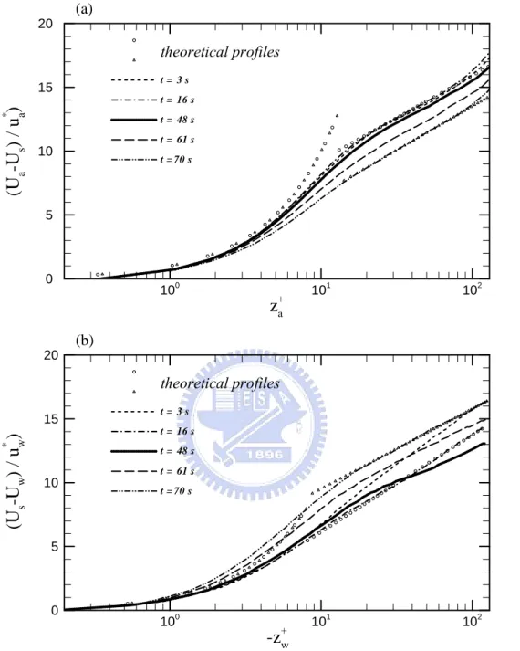
along with the theoretical profiles. Figure 14(a) shows that the simulated mean velocity

profiles in the air compare well with the theoretical two-layer velocity profile. When surface

But, when surface waves become significant (t>50s), wave motions change the mean velocity profiles, a systematic downward shift with time. This downward shift in the air

velocity profile is equivalent to an increase in surface roughness z (figure 16f), as ₀+ described in Sullivan et al. (2004), implying the enhancement of surface drag due to waves.

The surface roughness z is nearly constant ₀+ ~0.3 when t<50s and increases to about 95

.

0 when t~70s. The associated von Karman constant used to fit the logarithmic profile is about 0.33 at all time. Figure 14(b) shows the simulated mean velocity profiles and their

associated two-layer velocity profiles in the water. Not all profiles show the logarithmic

distribution and the von Karman constant κ is changing with time, 0.22<κ <0.36 when t < 24 s and 0.36<κ <0.44 when t > 24 s. (At t=3 s, the flow in the water may be too viscous as the mean wind profile is rather linear throughout.) The mean velocity profiles do not

undergo a systematic downward shift with time as in the air.

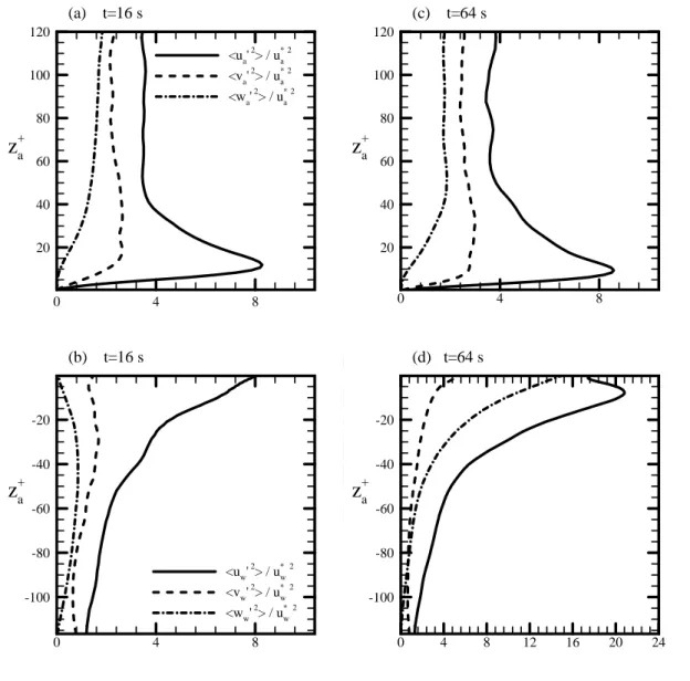
V.2 Wave effect on and turbulence intensities

The wave effect on the turbulent velocity variances is also different in air and water.

Figure 15 shows the turbulent velocity variances at two stages: t=16s when turbulence dominates (figure 15a and 15b) and t=64s when waves dominate (figures 15c and 15d). In the air, the vertical distributions of the velocity variances (normalized by the surface friction

velocity) 〈u′_i2〉(z)

( )

u∗_a 2 are in close agreement with wall-bounded shear turbulent flows (Kim et al. 1987, Aydin & Leutheusser 1991, Papavassiliou & Hanratty 1997 and Sullivan et

al. 2000). There is no significant change between turbulence and wave-dominated stages. In

the water, our profiles at t=16s agree with the stress-driven turbulent flow simulated by Tsai et al. (2005). However, at the stage when waves become significant, the velocity

variances in the water are strongly affected by waves, particularly the w component. The

horizontal-velocity variances near the interface also increase significantly due to waves. Such

an enhancement in the near surface turbulent velocity variances is attributed to the orbital

-z

+_w

(U

s

-U

w

)/

u

*

)

w 100 101 102 0 5 10 15 20 t = 3 s t = 16 s t = 48 s t = 61 s (b) theoretical profiles t = 70 s

z

+_a

(U

a

-U

s

)/

u

*

)

a 100 101 102 0 5 10 15 20 t = 3 s t = 16 s t = 48 s t = 61 s t = 70 s (a) theoretical profiles

Figure 14. Mean profiles of the streamwise velocity of the air (a) and water (b). The circular and delta symbols denote the matched linear-logarithmic profiles at t=16s and t=70s, respectively. The log-law constants used to collapse the profiles

( )

κ, z₀+ are (0.34, 0.31) and (0.33, 0.84) in the air and

( )

κ, z0+ are (0.3, 1.55) and (0.37, 0.3) in the water at time t =16s and t=70s, respectively.

0 4 8 20 40 60 80 100 120 (c) t=64 s z_a+ 0 4 8 12 16 20 24 -100 -80 -60 -40 -20 (d) t=64 s z_a+ 0 4 8 20 40 60 80 100 120 <u_a'2> / u*_a2 <v_a'2> / u*_a2 <w_a'2_{> / u}* a 2 (a) t=16 s z_a+ 0 4 8 -100 -80 -60 -40 -20 <u_w'2_{> / u}* w 2 <v_w'2> / u*_w2 <w_w'2> / u*_w2 (b) t=16 s z_a+

Figure 15. Vertical distributions of the normalized turbulent velocity variances of the air (upper panels) and of the water (lower panels) at early (t=16s) and later (t =64s) stages.

Chapter VI

Wave growth types

Previous theoretical studies suggest that wave growth processes can be separated into

linear and exponential growth stages and that the forcing mechanisms may involve either

turbulence-induced or wave-induced pressure and stress fluctuations. The consensus is that in

the linear growth stage, the wave-induced effects are ineffective since wave motions are weak

and thus turbulence plays a major role in generating waves. In the exponential growth stage,

wave-induced fluctuations of pressure and stress dominate and result in a feedback

mechanism to grow waves quickly. In this study, we examine the wave growth processes in

our simulated flow by classifying the simulation into linear and exponential wave-growth

stages using four features as follows.

First, the behaviour of pressure and shear stress fluctuations in the air is different at

early and later stages as described in section 3.2; they are turbulence dominated at early stage

and wave dominated at later stage. Second, the time evolution of the root-mean-square of

surface wave height 〈η2〉12 (figure 16a) clearly shows slow growth before t~40s and fast growth after t ~40s. Other statistical quantities, such as 〈p′_a2〉12, the form drag D , the _p mean surface current U , the root-mean-square of the interfacial shear-stress fluctuations _s

2 1 2〉 ′

〈τ_s and the surface roughness z (shown in figures 160+ b–f) also behave differently during early and late stages of the wave growth. They are nearly constant before t ~40s and then increase sharply with time. Third, the individual wave components of the fastest growing

modes given in Table 1 also reveal linear and exponential growth as shown in figure 17 where

the time evolutions of the wave amplitudes of the five fastest-growing waves in linear

coordinates for t<16s are shown in figure 17(a), and the three fastest-growing waves in exponential coordinates for 40< t<68s in figure 17(b). They clearly reveal trends of linear