高效能視訊編碼之標準制訂與運算平行化(I)

行政院國家科學委員會專題研究計畫 成果報告

高效能視訊編碼之標準制訂與運算平行化(I)

研究成果報告(精簡版)

計 畫 類 別 ： 整合型 計 畫 編 號 ： NSC 100-2221-E-009-073- 執 行 期 間 ： 100 年 08 月 01 日至 101 年 07 月 31 日 執 行 單 位 ： 國立交通大學資訊工程學系（所） 計 畫 主 持 人 ： 彭文孝 共 同 主 持 人 ： 杭學鳴 計畫參與人員： 碩士班研究生-兼任助理人員：陳彥宇 碩士班研究生-兼任助理人員：吳牧軒 碩士班研究生-兼任助理人員：蘇郁晴 碩士班研究生-兼任助理人員：朱弘正 碩士班研究生-兼任助理人員：吳昱興 碩士班研究生-兼任助理人員：王信硯 博士班研究生-兼任助理人員：陳俊吉 博士班研究生-兼任助理人員：吳崇豪 報 告 附 件 ： 出席國際會議研究心得報告及發表論文 公 開 資 訊 ： 本計畫可公開查詢

中 華 民 國 101 年 11 月 02 日

中 文 摘 要 ： 本報告提出一項單一區塊之多重動作向量預估模式，其同時 應用模塊樣板匹配 (Template Matching)與區塊動作補償 (Block Motion Compensation)兩種估測技術，輔以交疊區塊 動作補償(Overlapped Block Motion Compensation)技術有 效地結合兩種估測技術。透過模塊樣板匹配之動作向量可在 解碼端動態產生且不須耗費頻寬傳遞之特性，本技術只需傳 遞單一動作向量，搭配模塊樣板匹配之動作向量，即達到近 乎與傳統双動作向量估測相似的估測效能。透過兩種不同信 號模型的驗證，模塊樣板匹配之動作向量趨近於模塊樣板重 心點之運動向量。基於此，區塊動作向量搜尋的結果必需能 補償模塊樣板匹配估測效能不足之處；在我們的理論上，區 塊動作向量搜尋可視為在區塊(子)像素間挑出一者，以其動 作向量為最佳選擇套用至整個區塊上。此外，本文以實驗討 論壓縮效率與編解碼效率間的權衡，包含多模塊樣板類型之 測試、多動作向量預估模式、與簡化模塊樣板匹配之設計。 於 HM-3.0 軟體平台大量測試的結果證實了本文方法之效率與 可行性。 中文關鍵詞： 双動作向量估測、交疊區塊動作補償之預測、模塊樣板匹配 英 文 摘 要 ： This report introduces a multi-hypothesis temporal

prediction technique that combines two motion vectors (MVs) derived respectively from template and block matching for overlapped block motion compensation (OBMC). It achieves similar prediction performance to bi-prediction while only one MV has to be sent. Based on two signal models, the template MV is shown to approximate the pixel true motion around the template centroid. We then find another MV to best complement the template MV from both deterministic and

statistical viewpoints, the latter leading to the search of its optimal sampling location in the motion field. The result is a search criterion with OBMC window functions forming a geometry-like motion partitioning. To compromise between performance and complexity, generalizations to adaptive template design, multi-hypothesis prediction and motion merging are made. Extensive experiments conducted with the HM-3.0 software confirm the effectiveness of the proposed schemes.

英文關鍵詞： Bi-prediction, Overlapped Block Motion Compensation, Template Matching

行政院國家科學委員會專題研究計畫成果報告

高效能視訊編碼之標準制訂與運算平行化(I)

計畫類別：整合型 計畫編號：NSC100-2221-E-009-073 執行期限：100年08月01日至101年07月31日 主持人：彭文孝 教授 國立交通大學資訊工程系所 計畫參與人員：陳俊吉、吳崇豪、陳彥宇、吳牧軒、蘇郁晴、朱弘正、吳昱興、王信硯 _{國立交通大} 學資訊工程系所

中文摘要

本報告提出一項單一區塊之多重動作向量預估模式，其同時應用模塊樣板匹配 (Template

Matching)與區塊動作補償 (Block Motion Compensation)兩種估測技術，輔以交疊區塊動作補償

(Overlapped Block Motion Compensation)技術有效地結合兩種估測技術。透過模塊樣板匹配之動

作向量可在解碼端動態產生且不須耗費頻寬傳遞之特性，本技術只需傳遞單一動作向量，搭配模塊 樣板匹配之動作向量，即達到近乎與傳統双動作向量估測相似的估測效能。透過兩種不同信號模型 的驗證，模塊樣板匹配之動作向量趨近於模塊樣板重心點之運動向量。基於此，區塊動作向量搜尋 的結果必需能補償模塊樣板匹配估測效能不足之處；在我們的理論上，區塊動作向量搜尋可視為在 區塊(子)像素間挑出一者，以其動作向量為最佳選擇套用至整個區塊上。此外，本文以實驗討論壓 縮效率與編解碼效率間的權衡，包含多模塊樣板類型之測試、多動作向量預估模式、與簡化模塊樣 板匹配之設計。於HM-3.0軟體平台大量測試的結果證實了本文方法之效率與可行性。 關鍵詞：双動作向量估測、交疊區塊動作補償之預測、模塊樣板匹配

英文摘要

This report introduces a multi-hypothesis temporal prediction technique that combines two motion vectors (MVs) derived respectively from template and block matching for overlapped block motion compensation (OBMC). It achieves similar prediction performance to bi-prediction while only one MV has to be sent. Based on two signal models, the template MV is shown to approximate the pixel true motion around the template centroid. We then find another MV to best complement the template MV from both deterministic and statistical viewpoints, the latter leading to the search of its optimal sampling location in the motion field. The result is a search criterion with OBMC window functions forming a geometry-like motion partitioning. To compromise between performance and complexity, generalizations to adaptive template design, multi-hypothesis prediction and motion merging are made. Extensive experiments conducted with the HM-3.0 software confirm the effectiveness of the proposed schemes.

I. INTRODUCTION

A key issue in video coders with motion-compensated prediction is how to trade off effectively between the accuracy of the motion field representation and the required overhead. Often a rough representation of the motion field is sufficient to provide good temporal prediction in terms of rate-distortion (R-D) performance. Obvious evidences are the frequent occurrence of large motion partitions and of SKIP mode. Accordingly, many literatures related to the decoder-side motion vector derivation (DMVD) techniques are proposed, hoping to leverage the ever-increasing processing capability of the decoder to save motion overhead.

Template matching prediction (TMP) [4] is a well-known DMVD technique. It estimates the motion vector (MV) of a target block by minimizing the matching error over the reconstructed pixels in the template region, which is inverse-L-shaped and sitting on the top and to the left of the target block. Based on the concept, many of its variants have been proposed. Coding the target block at a lower spatial resolution followed by an interpolation was found more R-D efficient in flat areas, where TMP does not always guarantee to find a physically meaningful MV [10]. Even in non-flat areas, the template MV is merely a rough estimate of the target block’s motion. Hence, the multi-hypothesis prediction becomes popular to improve TMP [8]. Other alternatives include higher weight to pixels spatially closer to the target block when calculating the template matching error [3], and adapting the template shape and location to local signal characteristics [6].

Another school of thought follows multi-hypothesis TMP, but one of the hypotheses is sent as a coded MV. Apparently, how to optimize this MV is the key to its effectiveness. It is obtained by carrying out block matching as for BMC and then used as an initial estimate to confine template matching search [9]. However, this scheme is not guaranteed a minimal prediction residual, for it neglects the combined effect of involved predictors. To overcome this problem, our prior works [5] proceed in reverse order, resulting in less residual than TMP and BMC. Because the scheme is achieved with two hypotheses, it is viewed as a particular bi-prediction featuring only one coded MV.

The critical step of the above bi-prediction is the combination of predictors. A simple way is to compute their average [12]. In this report, we approach the problem from a theoretical perspective, assuming the use of the more general weighting scheme of overlapped block motion compensation (OBMC) [7]. Based on the underpinnings of [11] and [14], we show that the template MV is close to the true motion of a pixel near the top-left corner of the target block. A similar argument is then utilized to convert the problem of

finding a MV to best complement the template MV into the search for a certain pixel whose true motion will be served as the output, wherein the criterion is such that the mean-square prediction error over the target block will be minimized when applying these motion samples for OBMC.

Experiments based on the HM-3.0 software and common test conditions [1] confirm our bi-prediction to be effective. Several variants, which implement adaptive template switching with multi-hypothesis prediction or extend the notion to Motion Merging [13], were studied to trade off between performance and complexity. The best of them achieves 2.1-2.9% BD-rate savings at a cost of 34% and 44% increases respectively in encoding and decoding times. Replacing template matching by motion merging brings down the time increases to 19% and 3%, respectively, with BD-rate reductions dropping to 1.3-1.9% as a result. While this is by no means an ideal operating point, our work shows the potential of having the encoder and decoder work jointly to deliver better results.

The rest of this report is organized as follows: Section II analyzes TMP in a motion sampling framework. Within the framework, Section III formulates the optimal combination of TMP and BMC based on OBMC. Section IV evaluates the performance and complexity of the bi-prediction scheme and its variants. Section V concludes this report.

II. TEMPLATE MATCHING PREDICTION

In this section, TMP is studied to 1) reveal the factors that determine its prediction performance and 2) to understand its relationship to BMC.

A. Review of Signal Models

To analyze the residual of BMC, Tao et al. [11] modeled the autocorrelation functions of the intensity and motion fields by

[(s1)(s2)] = max µ 0 2_ µ 1 − ||s1− s2|| 2 2  ¶¶ (1a) [(s1)(s2)] = [(s1)(s2)] = 2ks 1−s2k1   (1b)

respectively, where (s) represents the intensity value of pixel s = ((s) (s)) of frame ; v(s) =

((s) (s)) denotes its true MV1; and {2 } and { 2

 } are parameters related to their respective

variances and correlation coefficients. Equations (1a) and (1b) suggest that the intensity and motion correlations between any two pixels decrease with the distance in between them.

1_{Under the constant intensity assumption, }

Similarly, in [14], Zheng et al. introduced a motion model assuming that the difference between the true MVs of any two pixels obeys the normal distribution:

(s1) − (s2) or (s1) − (s2) ∼ N (0 b2(s1 s2)) (2) where  is a constant indicating the degree of motion variation in the horizontal or vertical direction, and (s1 s2) =||s1− s2||2 is the 2 distance between pixels s1 and s2. The "hat" in (2) indicates that its value

will be clipped when exceeding a maximum threshold, which is essential for the model to be proper [2]. Equation (2) leads to the following autocorrelation function:

[(s1)(s2)] = [(s1)(s2)] = 2−

 2b

2_(s

1 s2) (3)

assuming the motion field is (wide-sense) stationary and zero-mean.

With these models, a closed-form expression for the mean-sqaure prediction error, [2_{(s; v(q))]where}

(s; v(q)) _{≡ }(s)−−1(s + v(q)), of pixel s based on the true MV of pixel q can be obtained. This

result is useful for analyzing various prediction schemes, as we shall see later. In [11], the derivation is done by a direct application of (1a) and (1b) in evaluating [(_−1(s + v(s))_{−−1}(s + v(q)))2], where, under the constant intensity assumption, _−1(s + v(s)) has been substituted for (s). This gives

[2(s; v(q))] = 8 2 2  ³ 1 − ||s−q||1  ´  (4)

Zheng et al. [14] take a different approach to find [2_{(s; v(q))], without the need of an intensity}

model. They approximate the prediction error by Taylor expansion, (s; v(q)) ≈ 0()

−1(s + v(q))((s)−

(q)) + _−10()(s + v(q)) ((s)− (q)), take expectation of the square of both sides, and assume the  

components of 0

−1(s + v(q)) and (v(s) − v(q)) are all independent of each other, to get

[2(s; v(q))] ∼= _b2(s q) ∼= _{||s − q||}2₂ (5)

where (2) is put into use and  = [(0()

−1(s + v(q))) 2

+ (_−10()(s + v(q)))2]. According to (4) and (5), several parallels between them can be drawn:

• The minimum of [2(s; v(q))] is reached when pixel q coincides with pixel s, which is obvious

from the constant intensity assumption.

• The value of [2(s; v(q))] increases when pixel q is further away from pixel s and converges to a

value proportional to 82

2 or , both have to do with the joint randomness of the motion and

intensity fields.

TABLE I

SAMPLINGLOCATIONS OFvFORVARIOUSTEMPLATECONFIGURATIONS

= 2 = 4 = 8

Block s (Block Center) Tao Zheng Tao Zheng Tao Zheng

4×4 (1.5,1.5) (-1,-1) (-0.25,-0.25) (-1,-2) (-1.25,-1.25) (-3,-3) (-3, -3)

8×8 (3.5,3.5) (-1,-1) (0.75, 0.75) (-1,-1) (0,0) (-2,-3) (-1.75,-1.75)

16×16 (7.5,7.5) (-1,-1) (2.75, 2.75) (-1,-1) (2,2) (-2,-2) (0.25,0.25)

(0,0) – the position of the top-left most pixel in the block B.  – the thickness of the template.

[2(s; v(q))] and the   components of (s − q), is mainly affected by the motion model. B. Sampling the Motion Field

With (5), a block MV, v, found from least-squares-based block matching was shown in [14] to

approximate the true motion associated with the block center, v(s), in the sense that the sum of prediction

error variances over the target block is minimized when v is chosen to be v(s):

s= arg min q X s∈B [2(s; v(q))] = Ã 1 |B| X s∈B (s) 1 |B| X s∈B (s) !  (6)

where B is a set consisting of coordinates of every pixel in the block. This can be easily verified by substituting (5) in (6) and setting the derivatives with respect to the   components of q equal to zero. A similar result is also observed with (4).2 _{Together these observations leads to an insightful interpretation}

of BMC: its operation may be viewed as a two-step process in which block-based motion estimation acts as a motion sampler taking samples at block centers while block-based motion compensation reconstructs the motion field by interpolating between motion samples using the nearest-neighbor rule .

Following the same line of derivation with B replaced by T and using (5), we have s =(

P

s∈T (s)|T |,

P

s∈T (s)|T |). Repeating the same computation with (4) gives a somewhat different result, but the trend

remains similar. Table I shows the locations of s. As can be seen, 1) the difference between v and v

can be view as their sampling locations in the motion field and 2) a change to the template configuration amounts to a variation of v’s sampling location.

C. Prediction Error Surfaces of BMC and TMP

With the background developed so far, we are now ready to proceed with exploring the distribution of prediction error variance over the target block B, termed the prediction error surface, for BMC and TMP. To do so, v and v are modeled by v(s) and v(s), respectively, and substituted for v(q) in (4) or (5)

2_{The optimal q in (6) cannot be found by differentation because of the }

1norm. We thus search exhaustively among all possible locations

(a) (b) (c)

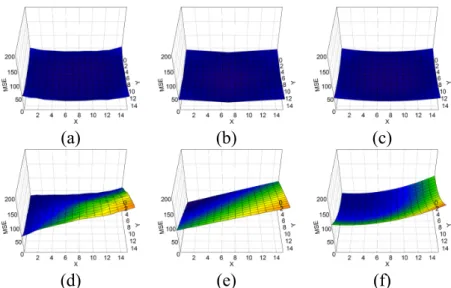
(d) (e) (f)

Fig. 1. Mean-square prediction error surfaces of block B produced with (a) BMC and (d) TMP. The second and third columns show the error surfaces predicted by Tao and Zheng’s models, respectively. (BasketballDrill, = = 16, = 4)

to compute the error variance for every pixel s in B. The results are visualized in Fig. 1 and compared with empirical surfaces that have been generated through real encoding.

The error surfaces of BMC, predicted respectively by the models, are convex shapes, whose minimum occur at the block center; in other words, the error variance tends to be smaller around the center and larger at block boundaries, which is understandable if we recall that v approximates v(s). Following the same

argument, the residual of TMP has a larger variance at the bottom-right quarter of the target block, because v, when viewed as v(s), generally has a weaker correlation to pixels’ true motion there. Comparing

these results with their empirical counterparts confirms the accuracy of our theoretical predictions. III. BI-PREDICTION COMBININGTMPAND BMC

A. Problem Formulation

The fact that in this application, v cannot be specified discretionarily by the encoder poses the key

question of what is then the most appropriate choice for v and the OBMC weights which, along with the

given v, would minimize the residual for every block. Obviously, we cannot afford to specify a unique

set of OBMC weights for each block, so the same weights must be shared among different blocks. Such restriction leads us to the following problem formulation:

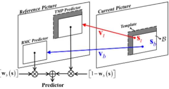
minimize v(s)(s)  =X ∈I X s∈B ((s) − (es) −1(s + v) − (es) −1(s + v))2

Fig. 2. Concept of bi-prediction combining TMP and BMC.

where s = ((s)(s)) is a pixel position relative to the top-left corner of a picture, with es = ((es)(es)) being its relative coordinates within a prediction block; {B}∈I denotes a set of those blocks in a picture

adopting this prediction scheme; and (es) and (es) are OBMC weights associated with the template

and block MVs, respectively. Note that an unconstrained equivalent of (7) can be obtained by substituting 1_{− }(es) for (es), leaving unknown only the block MVs, {v}∈I, and the corresponding OBMC

weights, (es).

B. Iterative Least-Squares (LS) Solution

The problem in (7) can be solved iteratively. Using an initial guess, called (0)

 (es), we can find a motion

vector v(0)

 for each prediction block B,  ∈ I, with the following search criterion

v_(0)= arg min v X s∈B ³ (s) − (1 − (0)(es))−1(s + v(0)) −  (0)  (es) −1(s + v) ´2  (8) where v(0)

 is computed right before the search of v (0)

 by performing TMP. Conditioned on the resulting

v(0)_ and v_(0), (es) is refined subsequently as follows for every distinct es:

(1)_ (_{es) =} P ∈I ³ (s) − −1(s+ v(0) ´ ³ −1(s+ v_(0)) − −1(s+ v(0)) ´ P ∈I ³ _−1(s+ v (0) ) − −1(s+ v (0) ) ´2  (9)

where s is a pixel in B. Then, the iteration continues by substituting the newly obtained  (1)

 (es) for

(0)_ (_{es) in (8). This procedure, although straightforward, is less instructive. We do not know the underlying} mechanism that gives rise to the solution, nor can we explain it.

C. Least Mean-Square (LMS) Solution

To gain more insights into the result, we transform the problem of minimizing the sum, , of squared prediction errors into that of minimizing its expected value, [], so that the aforementioned motion sampling concept and the signal models can come into play. Assuming that the intensity and motion

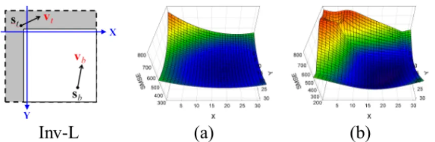
Inv-L (a) (b)

Fig. 3. Error surfaces showing how the sum of prediction error variances over the target block varies with the location of s: (a) Tao’s and

(b) Zheng’s models.

fields are stationary, the new objective becomes

minimize (s)s X s∈B h((s) − (1 − (es)) −1(s + v(s)) − (es) −1(s + v(s))) 2i  (10)

Obviously, for (10) to be minimized, the optimal (es) must satisfy, for all s ∈ B,

(es) =

[(s; v(s_))((s; v(s_{)) − (s; v(s})))]

[((s; v(s_{)) − (s; v(s}))2]  (11)

where (s; v(q))=(s)−−1(s + v(q)) q = s or s. Recall that from Table I, s is known once the

template shape and signal model are selected. Then, substituting (11) into (10), the summation is seen to be a function of  [(s; v(s_))2_{],  [(s; v(s}

))

2_{] and  [(s; v(s}

))(s; v(s))], and s is the last term to

be solved. Depending on which signal model is in use, the optimal s can be derived as

s∗_ = arg min s X s∈B 82 2  ⎛ ⎜ ⎝1 − ||s−s||1  − ³ 1 − ||s−s||1  − 1 + ||s−s ||1+ 1 − ||s−s||1 ´2 4³_{1 − }||s−s||1  ´ ⎞ ⎟ ⎠ (12)

with Tao’s model or

s∗_ = arg min s X s∈B  Ã b2_{(s s} ) − ¡ b2_{(s s} ) − b2(s s) +b2(s s) ¢2 4_b2_(s  s) ! (13)

with Zheng’s model. In particular, both equations suggest that there is no closed-form expression for s∗

–i.e., it has to be sought numerically.

Fig. 3 plots the sum of prediction error variances over the target block B as a function of s’s position,

with (0 0) being the position of the top-left pixel in B. The sum reaches the minimum when s∗

 sits in the

bottom-right quarter (see Table II for s∗

). As was noted before, TMP is less efficient in predicting pixels

in the bottom-right area. It is natural to expect the block MV to be so sampled as to compensate for its inefficiency. Once s∗

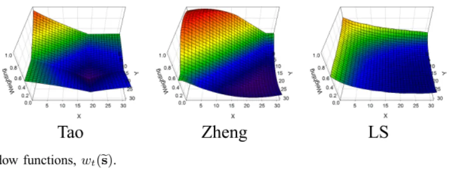
Tao Zheng LS

Fig. 4. Comparison of window functions, (s).

TABLE II

SAMPLINGLOCATIONS OFs∗FORVARIOUSTEMPLATECONFIGURATIONS

= 2 = 4 = 8

Block s(Block Center) Tao Zheng Tao Zheng Tao Zheng

4×4 (1.5, 1.5) (2, 2) (2, 2) (2, 2) (1.5, 1.5) (2, 2) (1.5, 1.5)

8×8 (3.5, 3.5) (5, 5) (4.5, 4.5) (5, 5) (4.5, 4.5) (4, 4) (4, 4)

16×16 (7.5, 7.5) (10, 10) (9.5, 9.5) (10, 10) (9.5, 9.5) (10, 10) (9, 9)

IV. EXPERIMENTALRESULTS

Experiments are carried out using the HM-3.0 software and common test conditions [1] to measure the coding performance of the proposed scheme (referred hereafter to as the TB-mode). A flag is sent for each non-skipped, 2Nx2N Prediction Unit (PU) to implement TB-mode as a switchable coding option. The search range for TMP is ±4 pixels and  = 4. The OBMC weights for the LS solution are computed

offline based on a separate set of training sequences, while the model parameters for the LMS solutions are selected empirically.3

A. Coding Performance

Table III shows the coding results of the LS and LMS solutions. In particular, three heuristic variants of the TB-mode, demonstrating the effects when v is estimated independently or dependently of v

and/or when a simple averaging of predictors is used in place of OBMC, are tested (Section _{2). These}

simple heuristics perform worse than the LS and LMS solutions (Section_{1); the straightforward approach}

(TB, 1/2), which simply averages the template and block predictors, even incurs 0.1% BD-rate increase. Incorporating OBMC (TB, LS) seems more beneficial than optimizing the block MV (TB, 1/2, ME opt.). But, neither approach comes close to the LS and LMS schemes, which deliver 0.7% in BD-rate reduction. All the schemes have almost the same level of encoding and decoding time increases. Their impact on encoding time (a 3-6% increase) is relatively modest, but the decoding time increase is still considerable (9-25%), mainly casued by performing TMP.

3_{For Tao’s model, }

= 095; for Zheng’s model, the clipping threshold is set equal to (2) 2

2with 2 denoting the width, or height, of the target PU.

TABLE III

COMPARISONS OFTB-MODES ANDTMP

Sec Mode Weighting ME Opt. RAHE RALC LBHE LBLC Avg. Enc. Dec.

TB LS o -0.7 -0.5 -0.8 -0.9 -0.7 106% 121% _{1 TB LMS-Tao o -0.7 -0.5 -0.7 -0.9 -0.7 106% 121%} TB LMS-Zheng o -0.7 -0.5 -0.8 -0.8 -0.7 106% 116% TB 1/2 0.0 0.0 0.1 0.2 0.1 103% 109% _{2 TB LS -0.3 -0.2 -0.3 -0.3 -0.3 103% 116%} TB 1/2 o -0.1 0.0 -0.1 -0.3 -0.1 105% 122%

Note – Negative values mean a rate reduction while positive values indicate a rate inflation. TABLE IV

COMPARISONS OFTB-MODES WITHFIXED ORVARIABLETEMPLATEPATTERN

RAHE RALC LBHE LBLC Avg. Enc. Dec.

(a) Fixed Template Pattern (Inverse-L) -0.7 -0.5 -0.7 -0.9 -0.7 106% 121%

(b) Variable Template Pattern -1.1 -0.9 -1.1 -1.5 -1.2 114% 119%

Note – The results shown are with Tao’s model and 2 hypotheses.

B. Adaptive Template Switching

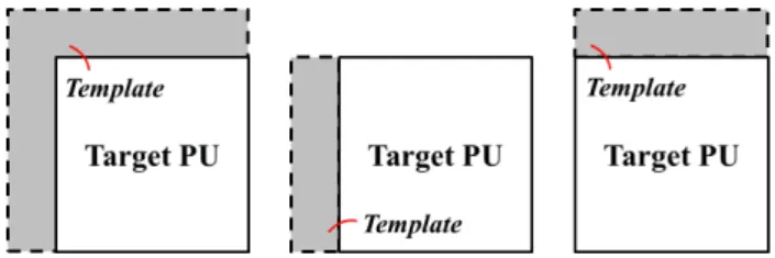
The coding performance of the TB-mode can improve at the cost of extra signaling overhead and computation. For instance, the encoder can switch between different template designs (see Fig. 5) to better adapt to time-varying signal characteristics. Of course, besides signaling the choice of template, the OBMC weights and block MV also need to be optimized by the same procedure described in Section III. From Table IV, this scheme further improves the rate saving by 0.4-0.6%, adding up to an average BD-rate saving of 1.2%, while elevating the encoding and decoding time ratios to 114% and 119%, respectively, due to extra computation needed for mode decision.

C. Multi-hypothesis Extension

The results given above have been generated by limiting the hypothesis number to two. Considering a three-hypothesis case, two block MVs, v1 and v2, and their associated OBMC weights, 1(es) and

2(es), has to be determined. More unknowns are to be solved, which largely complicates the iteration

process of the LS solution, so we resort to the LMS approach. In analogy with (10), the objective is to find two pixels, s1 and s2, in the target block B that minimize:

 =X s∈B ∙³ _{(s) − (es) −1(s + v(s} ))−1(es) −1(s + v(s1)) −2(es) −1(s + v(s1)) ´2¸  (14)

where v, v1 and v2 are modeled, respectively, by v(s) v(s1) and v(s2) with s as a priori, and

(es) = 1 − 1(es) − 2(es). Proceeding in much the same way as in [2], we can solve for the solution,

s∗

1 and s∗2, by evaluating  for all permissible values of s1 s2∈ B, which involves only the second-order

moments of (s; v(s_)) (s; v(s_1)) (s; v(s_2)).4 Using the result, v1 and v2 are then estimated by

4_{Refer to (6) and (11) in [2] for evaluating  }

Fig. 5. Adaptive template switching.

divide-and-conquer, with v1 first found by

v_1∗ = arg min

v1

X

s∈B

((s) − (1 − 1∗ (es; s s∗1)) −1(s + v) − 1∗ (es; s s∗1) −1(s + v1))2 (15) and utilized subsequently alone with v to find v2 as follows:

v∗2= arg min v2 X s∈B ⎛ ⎝ (s) − (1 − ∗1(es; s s∗1 s∗2) − ∗2(es; s s∗1 s∗2)) −1(s + v) −∗1(es; s s∗1 s∗2) −1(s + v∗1) − ∗2(es; s s∗1 s∗2) −1(s + v2) ⎞ ⎠ 2  (16) where the ∗

1(es) and ∗2(es) are augmented with the sampling points (s, s∗1 or s∗2) from which they

are computed.5

We also preserve the flexibility of TB-mode to switch between two- and three-hypothesis cases, in order to be R-D effective. However, the s∗

1 in (14) is generally not equal to s∗ in (10), resulting in three times

of motion search respectively for v∗

, v∗1, and v2∗ . To reduce the complexity, we simply let s∗1= s∗2= s∗,

resulting in ∗

1(es) and 2∗ (es) equal to 1

2∗(es). Hence, there is no need to find v∗1 since its result is

exactly identical to v∗ .

Table V compares the results of TB-modes with varying the numbers of hypothesis. Note that the notation, taking Experiment (b) as an example, (1 v+ 2 v’s) means that the encoder can choose adaptively

the TB-mode with (1 v+ 1 v) or (1 v+ 2 v’s). In (b) and (e), there is almost no difference, in terms of

BD-rate savaings, between the heuristic and theoretically optimal approaches. Only 0.1-0.2% rate saving in the low-delay conditions is obtained from the optimal approach, while increasing the encoding time by 10% which is nearly unacceptable. Hence, we adopt the heuristic approach for the later experiments.

From the table (a-d), increasing the maximum hypothesis number from 2 to 4 almost doubles the rate saving in every test condition, achieving an average BD-rate reduction of 2.2%, and the increase of decoding time is about 30% higher than the (1 v + 1 v). As it stands, the setting (1 v + 2 v’s) seems

to offer a better compromise between performance and complexity, with a comparable encoding/decoding time increase to (1 v + 1 v), yet a moderate rate saving (1.8%, on average). The same observation does

5_s∗

TABLE V

COMPARISONS OFTB-MODES WITHMULTI-HYPOTHESISPREDICTION

Hypotheses Heuristic RAHE RALC LBHE LBLC Avg. Enc. Dec.

(a) 2 (1 v + 1 v) -1.1 -0.9 -1.1 -1.5 -1.2 114% 119%

(b) 3 (1 v + 2 v’s) o -1.6 -1.6 -1.7 -2.2 -1.8 119% 125%

(c) 3 (2 v’s + 1 v) -1.6 -1.4 -2.0 -2.4 -1.8 118% 143%

(d) 4 (2 v’s + 2 v’s) o -2.0 -1.9 -2.2 -2.7 -2.2 122% 147%

(e) 3 (1 v + 2 v’s) -1.6 -1.5 -1.8 -2.4 -1.8 129% 125%

Note – The results shown are with adaptive template switching. TABLE VI

COMPARISONS OFTB-MODES WITHMOTIONMERGING

Hypotheses RAHE RALC LBHE LBLC Avg. Enc. Dec.

(a) 2 (1 MRG v+ 1 v) -0.7 -0.5 -0.9 -0.8 -0.7 106% 101%

(b) 3 (1 MRG v+ 2 v’s) -0.9 -0.8 -1.2 -1.3 -1.1 110% 102%

(c) 3 (2 MRG v’s + 1 v) -0.9 -0.7 -1.2 -1.2 -1.0 108% 102%

(d) 4 (2 MRG v’s + 2 v’s) -1.1 -1.0 -1.3 -1.5 -1.2 109% 103%

not apply to the other 3-hypothesis scheme, (2 v’s + 1 v), which differs in using more v’s. For this

reason, its decoding time increase is as considerable as (2 v’s + 2 v’s).

D. Generalization to Motion Merging

The idea of Motion Merging [13] is to send few bits to reuse MV(s) from a previously decoded neighboring PU as v. It is similar to treating the motion sample taken at the center of the referred

PU as v, in which case selecting adaptively from a range of candidate PUs is assimilated to switching

between different template designs. In this analogy, we simply apply the previous OBMC windows to the present case, and the weight values are rounded to power-of-two numbers with 3-bit integer precision for simplification. Comparing Table VI with Table V, the performance declines 0.5-1.0% across different experiments, but also much lower encoding and decoding time increases. The high complexity associated with TMP can be thus resolved. Performance loss may be inevitable; it however can be mitigated without significantly complicating the decoder.

V. CONCLUSION

We proposed a bi-prediction scheme combining BMC and TMP predictors through OBMC. First, TMP is examined in the context of motion field sampling and showed that the template MV may be viewed as the pixel true motion around the template centroid. Following a similar argument, we formulated the problem of finding an MV to best complement the template MV as the search of its sampling location in the motion field. This formulation allows solving the problem analytically and leading to useful insights into the solution. We found that when sampled optimally, this MV, along with the template MV, forms

a geometry-like motion partitioning. The notion of our scheme is capable of tremendous generalization. The template pattern need not be fixed, the number of hypotheses can be extended over two, and TMP can be replaced with other DMVD techniques, such as Motion Merging. Experimental results confirm our scheme to be effective.

REFERENCES

[1] F. Bossen, “Common test conditions and software reference configurations,” Doc. JCTVC-E700, 2011.

[2] Y. W. Chen and W. H. Peng, “Parametric OBMC for Pixel-Adaptive Temporal Prediction on Irregular Motion Sampling Grids,” IEEE Trans. on Circuits and Systems for Video Technology, vol. 22, no. 1, pp. 113–127, Jan. 2012.

[3] Y. W. Huang et al., “TE1: Decoder-side motion vector derivation with switchable template matching,” Doc. JCTVC-B076, 2011. [4] S. Kamp et al., “Decoder Side Motion Vector Derivation for Inter Frame Video Coding,” Proc. Int’l Conf. on Image Processing, 2008. [5] C. L. Lee et al., “Bi-prediction Combining Template and Block Motion Compensations,” Proc. Int’l Conf. on Image Processing, 2011. [6] S. Lin et al., “TE1: Huawei report on DMVD improvements (joint document with Peking University),” Doc. JCTVC-B037, 2010. [7] M. T. Orchard and G. J. Sullivan, “Overlapped block motion compensation: An estimation-theoretic approach,” IEEE Trans. on Image

Processing, vol. 3, no. 5, pp. 693–699, Sep. 1994.

[8] S. Kamp and others, “Multihypothesis prediction using decoder side motion vector derivation in inter frame video coding,” Visual Comm. and Image Processing, 2009.

[9] Y. Suzuki and C. S. Boon, “An improved low delay inter frame coding using template matching averaging,” Proc. Picture Coding Symposium, 2010.

[10] Y. Suzuki et al., “Block-based reduced resolution inter frame coding with template matching prediction,” Proc. Int’l Conf. on Image Processing, 2006.

[11] B. Tao and M. T. Orchard, “A parametric solution for optimal overlapped block motion compensation,” IEEE Trans. on Image Processing, vol. 10, no. 3, pp. 341–350, Mar. 2001.

[12] R. Wang et al., “Combining Template Matching and Block Motion Compensation for Video Coding,” in Proc. Int’l Symp. on Intelligent Signal Processing and Communication Systems, 2010.

[13] M. Winken et al., “Description of Video Coding Technology Proposal by Fraunhofer HHI,” Doc. JCTVC-A116, 2010.

[14] W. Zheng et al., “Analysis of space-dependent characteristics of motion-compensated frame differences based on a statistical motion distribution model,” IEEE Trans. on Image Processing, vol. 11, no. 4, pp. 377–386, Apr. 2002.

行政院國家科學委員會補助國內專家學者出席國際學術會議報告

101 年 10 月 25 日 報告人姓名 彭文孝 服務機構 及職稱 國立交通大學資訊工程學系 助理教授 時間 會議 地點 101 年 5 月 20 日至 101 年 5 月 23 日 南韓首爾 本會核定 補助文號 會議 名稱 (中文) 2012 國際 IEEE 電路與系統研討會

(英文) 2012 IEEE International Symposium on Circuits and Systems 發表

論文 題目

(中文) 針對可調視訊編碼粗略可調性之模式相依的位元與失真解析模型 (英文) Analytical Mode-Dependent Rate and Distortion Models for H.264/SVC Coarse Grain Scalability

報告內容應包括下列各項： 一、參加會議經過

2012年國際IEEE電路與系統(IEEE International Symposium on Circuits and Systems)研討會於5月20日至5月23日在南韓首爾舉行，本屆ISCAS＇2012 共計有1,760 篇論文投稿，最後接受來至世界各地822篇論文發表，接受率約46%，依論文特色與領域 共分成31個技術主題之場次，分173個平行場次進行，同時本次研討會在議程的設計上， 除了一般性的論文發表外，大會亦特別安排了三場Keynote Speeches，分別介紹三個極 具潛力及前瞻性的研究領域，聆聽三位大師的演講，不僅瞻仰大師的丰采，亦提升了筆 者於學術領域的廣度，著實獲益良多。 在四天的議程安排中，大會並聘請多位專家學者針對電路與系統相關領域的特定主 題安排 10 場訓練課程(Tutorials)，主題分別為：(1) Practical ESD Protection Co-design Techniques for ICs, Modules, and Systems、(2) Digital Delta-Sigma Modulators for DAC and Fractional-N Frequency Synthesis Applications、(3) Smart CMOS Image Sensors for 2-D and 3-D Capture and Processing: Pixels, Circuits, Architectures, and Practical Design Guidelines 、 (4) Smart Grids, Electric Vehicles, and Energy Storage Systems: Emerging Trends, Circuits, and Devices、 (5) Computer Algebra and Its Applications to Circuits, Signals, and Systems、 (6) On-chip High-voltage Generator Design、(7) High-/Mixed-Voltage Analog and RF Circuits and Systems for Wireless Applications、(8) Advances in Speech Coding, Speech Recognition, and Applications、(9) Small Scale Energy Harvesting (EH) – Principles, Practices, and Future Trends、(10) Challenges and Opportunities in Internet of Things。所安排的訓練課程內容涵蓋數位、類比與射頻電路與系統，影像、 視訊處理與壓縮，不但針對相關技術的介紹，亦加強系統設計上的整體考量。其餘三天 為論文口頭報告（Lecture Session）與壁報發表（Poster Session），總共包含 16 個 技術主題（Tracks），共 173 場次分 117 個口頭報告場次及 56 個壁報發表場次同時進 行，與會者可依興趣與專長選擇適合的場次聽講及發問。其中 16 個主題分別為：(1) Analog Signal Processing、(2) Biomedical and Life Science Circuits, Systems and 、(3) Circuits and Systems for Communications、(4) Computer-Aided Network Design、(5) Digital Signal Processing、(6) Multimedia Systems and Applications、

附

件

(7) Nanoelectronics and Gigascale Systems、(8) Neural Networks and Systems、 (9) Nonlinear Circuits and Systems、(10) Power Systems and Power Electronic Circuits 、 (11) Sensory Systems 、 (12) Visual Signal Processing and Communications 、 (13) VLSI Systems, Architectures and Applications 、 (14) Education in Circuits and Systems 、 (15) SPECIAL SESSIONS 、 (16) Live Demonstrations of Circuits and Systems。

筆者於會議期間遇到不少來至台灣產、學界的學者如本校張天烜教授、聯發科技的 劉子明博士等，更加深他鄉遇故知之感覺，更可感覺到台灣學術界在此領域之參與度不 斷的提升及在此會議之影響力，也對來自台灣多位學者於此會議之貢獻感到驕傲。與會 期間亦認識歐美與中港新加坡等地的學者如德國漢諾威大學Jörn Ostermann教授，不但 領受學術之交流，亦感覺到主辦單位籌備之用心，讓每位參與者皆有賓至如歸之感覺。 二、與會心得 IEEE 電路與系統國際研討會為一歷史悠久，且其規模亦不斷成長的國際著名研討會， 最近幾年輪流由於歐洲、澳洲、亞洲、美洲等地舉行，真是實至名歸的國際研討會。此 研討會集合從事多媒體訊號處理相關之專家學者與研究人員，交換研究心得、工作經驗 與學、業界發表，更是視訊壓縮、影像處理等領域重要的年度盛事之一。對於從事相關 研究的學者而言，每年的參與應可獲得相當程度的幫助，同時亦於第一時間接觸到最新 且最熱門研究主題(例如：高效能視訊壓縮、3D 視訊壓縮)。整體而言，此會議所包含的 研究領域廣泛（每年似乎皆有成長，足可見相關應用之多元化發展）、論文內容豐富且 質精，是一非常值得參加的會議。筆者此次參加此會議，不僅皆獲得不少與本人研究相 關的知識，更獲得同領域學者於學術研究上的建議與新知。很幸運可於與會同時認識了 多位國內外相關領域之學者，對於知識的擴展與友誼的增進方面均覺受益良多，實已達 到了學術交流之目的，在此特別感謝國科會所給予之補助。 此外，由每年來至台灣的參與學者及所發表的論文總數而言，可見台灣在積體電路 設計的研究與發展已具備相當程度的國際競爭力，足見政府於學術領域的深耕與努力是 非常值得的。 三、考察參觀活動(無是項活動者省略) 無。 四、建議 基於參與此次 ISCAS’2012 會議的經驗，筆者之建議如下：因為第一天的訓練課程常 常有一些是參與學者非常有興趣參加的，因主講者針對演講之主題所整理的資料，通常 不但具有一定程度的啟發性與前瞻性，並且有助於個人研究，亦可能提供為未來之教學 教材內容，若能將參與訓練課程之費用也列入補助項目，將是一非常正面且實質的鼓勵。 五、攜回資料名稱及內容 本次會議所有的論文皆收錄在一片光碟內，每一位與會學者皆可擁有一片。筆者所 攜回之資料為：(1)ISCAS’2012 CD 論文集一片、(2)ISCAS’2012 會議導覽手冊一本(2) 近期相關領域之論文徵稿資料。 六、其他 無。

國科會補助計畫衍生研發成果推廣資料表

日期:2012/10/31

國科會補助計畫

計畫名稱: 高效能視訊編碼之標準制訂與運算平行化(I) 計畫主持人: 彭文孝 計畫編號: 100-2221-E-009-073- 學門領域: 積體電路及系統設計

無研發成果推廣資料

100 年度專題研究計畫研究成果彙整表

計畫主持人：彭文孝 計畫編號： 100-2221-E-009-073-計畫名稱：高效能視訊編碼之標準制訂與運算平行化(I) 量化 成果項目 實際已達成 數（被接受 或已發表） 預期總達成 數(含實際已 達成數) 本計畫實 際貢獻百 分比 單位 備 註 （ 質 化 說 明：如 數 個 計 畫 共 同 成 果、成 果 列 為 該 期 刊 之 封 面 故 事 ... 等） 期刊論文 0 0 100% 研究報告/技術報告 0 0 100% 研討會論文 0 0 100% 篇 論文著作 專書 0 0 100% 申請中件數 0 0 100% 專利 已獲得件數 0 0 100% 件 件數 0 0 100% 件 技術移轉 權利金 0 0 100% 千元 碩士生 0 0 100% 博士生 0 0 100% 博士後研究員 0 0 100% 國內 參與計畫人力 （本國籍） 專任助理 0 0 100% 人次 期刊論文 1 1 100% 研究報告/技術報告 0 0 100% 研討會論文 2 2 100% 篇 論文著作 專書 0 0 100% 章/本 申請中件數 0 0 100% 專利 已獲得件數 0 0 100% 件 件數 0 0 100% 件 技術移轉 權利金 0 0 100% 千元 碩士生 0 0 100% 博士生 0 0 100% 博士後研究員 0 0 100% 國外 參與計畫人力 （外國籍） 專任助理 0 0 100% 人次

其他成果

(

無法以量化表達之成 果如辦理學術活動、獲 得獎項、重要國際合 作、研究成果國際影響 力及其他協助產業技 術發展之具體效益事 項等，請以文字敘述填 列。) 一、擔任國際性學術組織技術主席

(1) 2011, 未來數位視訊研討會 Future Video Workshop

(2) 2011, IEEE Visual Communications and Image Processing 二、擔任國際性學術組織技術委員

(1) 2011 and 2012, IEEE Visual Communications and Image Processing (2) 2011 and 2012, IEEE International Symposium on Circuits and Systems 三、群體計畫子項主持人 (1) 2011 and 2012, 多媒體標準(MPEG)資源共享計畫 成果項目 量化 名稱或內容性質簡述 測驗工具(含質性與量性) 0 課程/模組 0 電腦及網路系統或工具 0 教材 0 舉辦之活動/競賽 0 研討會/工作坊 0 電子報、網站 0 科 教 處 計 畫 加 填 項 目 計畫成果推廣之參與（閱聽）人數 0

國科會補助專題研究計畫成果報告自評表

請就研究內容與原計畫相符程度、達成預期目標情況、研究成果之學術或應用價

值（簡要敘述成果所代表之意義、價值、影響或進一步發展之可能性）

、是否適

合在學術期刊發表或申請專利、主要發現或其他有關價值等，作一綜合評估。

1. 請就研究內容與原計畫相符程度、達成預期目標情況作一綜合評估

■達成目標

□未達成目標（請說明，以 100 字為限）

□實驗失敗

□因故實驗中斷

□其他原因

說明：

2. 研究成果在學術期刊發表或申請專利等情形：

論文：■已發表 □未發表之文稿 □撰寫中 □無

專利：□已獲得 □申請中 ■無

技轉：□已技轉 □洽談中 ■無

其他：（以 100 字為限）

3. 請依學術成就、技術創新、社會影響等方面，評估研究成果之學術或應用價

值（簡要敘述成果所代表之意義、價值、影響或進一步發展之可能性）（以

500 字為限）

一、學術成就

本年度共發表 1 篇期刊論文與 2 篇研討會論文，分別提出(1)Motion Uncertainty 於 Motion Sampling 上之分析，並分析出動作估測時, 動作向量於區塊中的理論位置，提升 POBMC 於動作補償時的準確性。(2)提出針對可調視訊編碼粗略可調性之模式相依的位元與失真 解析模型。(3)提出一多重動作向量預估模式，同時利用 TMP 與 BMC 區塊估測技術，輔以 OBMC 技術有效地結合兩者，提升現有 HEVC 之編碼效率。

[1] Y. W. Chen and W. H. Peng, ＇＇Parametric OBMC for Pixel-Adaptive Temporal Prediction on Irregular Motion Sampling Grids,＇＇ IEEE Transactions on Circuits and Systems for Video Technology, vol. 22, no. 1, pp. 113-127, January 2012. [2] C. H. Wu, Y. C. Tseng, and W. H. Peng, ＇＇Analytical Mode-Dependent Rate and Distortion Models for H.264/SVC Coarse Grain Scalability,＇＇ Proc. IEEE International Symposium on Circuits and Systems, ISCAS-2012, Seoul, Korea, May 2012.

[3] C. L. Lee, C. C. Chen, Y. W. Chen, M. H. Wu, C. H. Wu and W. H. Peng, ＇＇Bi-prediction Combining Template and Block Motion Compensations,＇＇ Proc. IEEE International Conference on Image Processing, ICIP-2011, Brussels,

二、技術創新 結合模塊樣板匹配預測、區塊動作補償及其交疊區塊動態補償，有效提高動作估測的正確 性。此外，本技術只需傳遞單一動作向量，並搭配模塊樣板匹配之動作向量，即達到近乎 與傳統双動作向量估測相似的估測效能 三、社會影響 本計畫發表了許多具有學術價值的成果，其中在國際標準會議上也有貢獻，並藉此機會培 育出許多視訊壓縮領域之人才，主要由兩位博士生與一位碩士生參與計畫核心演算法之開 發與執行，參與計畫之研究人員亦獲得了許多視訊壓縮相關之最新技術之設計經驗，不論 是對學術相關研究或是與國內業界合作進行相關產業之新產品開發，都有正面的價值。