行政院國家科學委員會專題研究計畫 期中進度報告
無線通訊系統及定位系統的傳播研究及天線設計(1/2)
計畫類別: 個別型計畫
計畫編號: NSC93-2213-E-002-092-
執行期間: 93 年 08 月 01 日至 94 年 07 月 31 日
執行單位: 國立臺灣大學電信工程學研究所
計畫主持人: 江簡富
報告類型: 精簡報告
處理方式: 本計畫可公開查詢
中 華 民 國 95 年 2 月 27 日
無線通訊系統及定位系統的傳播研究及天線設計(1/2)
NSC 93-2213-E-002-092
PI: Jean-Fu Kiang
Department of Electrical Engineering and Graduate Institute of Communication Engineering
National Taiwan University
No.1, Sec. 4, Roosevelt Road, Taipei, Taiwan, ROC
The contents of this annual report consist of three parts. The first part, “scattering analysis of large metallic bodies” summarizes a propagation model for vehicles moving around a base station, the second part, “dielectric-resonator-fed active horn antenna” summarizes the design of a directional horn antenna using ceramic material, the third part, “dual-band dielectric resonator antenna” presents a miniaturized ceramic antenna.
Scattering Analysis of Large Metallic
Bodies
Abstract — A hybrid full-wave analysis procedure is developed by utilizing the information of scatter surfaces. Equivalent currents are derived with hybrid methods and used to calculate the scattering fields. A scaled model is also built and measured to verify our approach. The results of simulation and measurement match reasonably well. This approach is practical and computationally efficient.
Key Words — channel analysis, equivalent current,
hybrid method, large object, metallic bodies, scattering analysis, vehicular communication.
I. INTRODUCTION
The demands of wireless communication, such as cellular phones, wireless LAN and WiMax, largely increase in the past ten years, and the trend also affects the transportation industry. Intelligent transportation system (ITS) is proposed in response to the growing demands for mobility, safety, limited road capacities, and so on. The core of such system is the exchange of information to and from the vehicles. Such communication between the roadside infrastructure and vehicles can be carried out over roadside beacons with a bidirectional data link.
The performance of a wireless communication system strongly depends on the channel it experiences. If the medium is well characterized, the transmitter and receiver can be designed to match the channel and reduce the effects of disturbances. In a roadside-to-vehicle application, the transmitters and receivers may have relative motions. Due to reflection, refraction and scattering of radio waves by buildings, hills, and other objects, the signals will suffer from multipath fading. The receiving signal is a distorted version of the original
signal, incorporating a possible direct signal and indirect signals from ground reflection, scattering from roadside buildings and moving vehicles, and so on. Traditionally, such communication channels are usually described with statistical parameters. These parameters and the associated formulas, such as Rayleigh and Rican models, can describe the channel on the average, but the real-time physical situation only loosely links to the parameters. In this work, a full-wave analysis procedure is developed with the fundamental ideas of equivalent currents, based on which a numerical program is developed and measurements are done to verify this approach.
II. ANALYSIS OF SECENARIO
The communication systems in this work are targeted for wireless, outdoor, and vehicular use. Performance of such communication links is affected by many factors, including signal modulation, encryption, interleaving, bandwidth of signals, vehicular speed, distribution of scatterers, base station distributions, geographical changes, weather, and so on. Due to wireless and outdoor environments, there are always a large number of scattering signals. These scattering signals propagate over different paths and result in multipath effects on the receivers.
Consider an open area without roadside objects to perform analysis. Antenna arrays can be used to shape the radiation patterns to focus on a specific part of the road. Hence, the communication area is restricted and the number of paths can be reduced for analysis. One of major paths is the ground reflection which has almost the same power level as the line-of-sight signal. There are also scattering signals from nearby vehicles. Because vehicle bodies are mainly made of metal, strong scattering waves will be incurred as a wave incides upon a vehicle. Nearby receivers may receive some scattering signal, rendering noises or signal fluctuation to the desired signal.
III. DEVELOPMENT OF CHANNEL MODEL
The multipath signals can be categorized into three types due to the characteristics of signal propagation: line-of-sight, ground reflection, and scattering signal as shown in Fig.1. The line-of-sight signal propagates between the transmitter and the receiver without obstruction. The received field depends on the antenna type, propagation distance, polarization and transmitter
power. Because the transmitter is located at the roadside base station, the LOS field is the far-field from the transmitting antenna. The ground is assumed to be a large plane, and the reflected signal is approximated by ray-asymptotic approach. The characteristics of the scattering field from a surface depends on the surface properties and the incident field. Table 1 shows the relative permittivity and conductivity of several surfaces [2].
Thin-wire Panel Edge Ground LOS Tx Rx Z X Y
Figure 1: Scattering scheme of the problem scenario.
Table 1. Typical electrical surface of different surfaces [2]
Type of Surface σ(Siemens/m) εr
Poor Ground 0.001 4
Average Ground 0.005 15
Good Ground 0.02 25
Sea water 5 81
Fresh water 0.01 81
Besides of the line-of-sight signal and the ground reflected signals, the received signals also include the signals scattered by nearby objects. Since our scenario focuses on the open area, the main contributor of the scattering signal is the car body near the receiver. In order to calculate the scattered field of a vehicle, the car body surface is decomposed into three types of components: panels, edges, and thin wires. Rooftops, side doors and hoods are categorized as panels, and the connections of panels are categorized as edges. Window supports, bumpers and similar structures are modeled as thin wires. In this work, a Volvo-740 is chosen as our reference model. Its overall length is 4.785 meters and overall width is 1.75 meters. The carrier frequency in our simulation is set around 900 MHz with a free-space wavelength about 33 cm.
In the analysis, equivalent current approach is used to calculate the scattering field of the object. When an electromagnetic wave incides upon an object, there are induced currents and charges on the surface and scattering fields outside the object. These currents and charges can be viewed as the secondary sources which result in the scattering fields. The vector potential associated with the induced current can be written as
| '| 0 ( ') ( ) ' 4 | jk r r S S J r e A r dr r r µ π − − = −
∫∫
' |where JS( )r is the surface equivalent current. The far-field scattering far-fields can be approximated as
ˆˆ ( ) E= −jω A− iA kk 0 1 ˆ H k η E = ×
where is the propagation direction of the scattered wave. When the integral in
ˆk
A is calculated numerically, the trade-off between accuracy and computation time is unavoidable. However, some skills are incorporated in the simulation to speed up the calculation while maintain same level of accuracy.
Panels are large flat areas on the vehicular surface. Imposing the boundary condition, the surface current,
S
J
, can be modeled asˆ
2
ˆ
S total inc
J
= ×
n H
≈
n H
×
where
H
inc is the incident magnetic field. As shown in Fig.2, a large panel is divided into small rectangular panels. The scattering field of each piece is summed up to obtain the total scattering field. The size of each panel is based on the far-field criteria, and closed-form expression for the far-field can be applied.E, H
Figure 2: Slice the panel to satisfy the far field contition.
With this additional slice procedure, the total computation time is reduced because the scattered fields of each panel are calculated using closed form far-field equation of a rectangular panel.
The edge connecting two panels is modeled as a one-fourth cylinder with the cross section of a 90°-circular sector. The radius of curvature is much smaller than one wavelength. Thus, when the electromagnetic wave is impinging upon the edge, the scattered field will be very similar to the diffraction by a sharp wedge. The diffracted field solutions based on the uniform geometric theory of diffraction (UTD) has been developed and continuously improved since 1976 [5], [6]. The results described in the UTD are the asymptotic far-field solutions. However, the situation in our simulation is not quite so. For example, the observation point is not far enough to apply the solution of UTD directly to the whole edge. In our approach, assume that there exist equivalent electric and magnetic currents along the edge. Then, the scattered field is calculated using the associated vector potential. By similar process as for the panel, the edge is first sliced into smaller sections so that the UTD closed-form far-field solutions can be applied directly to compute the equivalent currents on the edge. The total scattering field is the summation of the radiation fields by these equivalent currents.
Me Ie
Figure 3: Schematic of edge analysis process.
Because the cross-sectional size of the support is smaller than a carrier wavelength, the widow supports are modeled as thin wires. The magnitudes of the equivalent currents on the thin wire depend on the boundary condition and the incident wave. For a straight thin wire located at the origin of the coordinate system as shown in Fig. 4, the surface current can be expressed as [7]
1 cos , (2) 0 2( sin ) ˆ ( ) { ( sin ) i jkz n i TM S TM n n i ka E J z z e j H ka θ π θ η θ − ∞ − =−∞ = −
∑
− 2 'cos [cos ( sin ) ( sin )]} jn i J kan i J kan i e φ θ φ θ θ + − 1 cos , (2)' 0 2( sin ) ˆ ( ) sin ( sin ) i jkz n i j TE S TE i n n i ka H n J z e j H ka θ e φ π θ φ θ η θ − ∞ − =−∞ =
∑
x z y E , H i θFigure 4: Scenario of a thin wire scattering.
IV. SIMULATIONS AND MEASUREMENTS
The measurements are conducted in an anechoic chamber of size 5.8 m x 10 m x 5 m. Two standardized horn antennas, which can operate from 1 to 18 GHz, are used as the transmitting and the receiving antennas. The scatterer is a 10-to-1 model of the Volvo 740 GLE sedan. The vehicle model is made of carton board and covered by copper foil, and the windshield supports and four hubcaps are also covered by copper foil. The setting of the experiment is shown in Fig. 5. The operating frequency is set as 9 GHz, scaling to the scattering of a full-size vehicle at 900 MHz. The transmitting antenna and the receiving antenna are placed on the same horizontal level with both main beams pointing at the scatterer located on the rotation pedestal. The distance between the transmitting antenna and the scatterer is 6 m, and the distance between the scatterer and the receiving antenna is 1.2 m. The two paths are arranged to be perpendicular to reduce the effect of the line-of-sight signal.
Tx
Rx
Figure 5: Setting of the experiment environment.
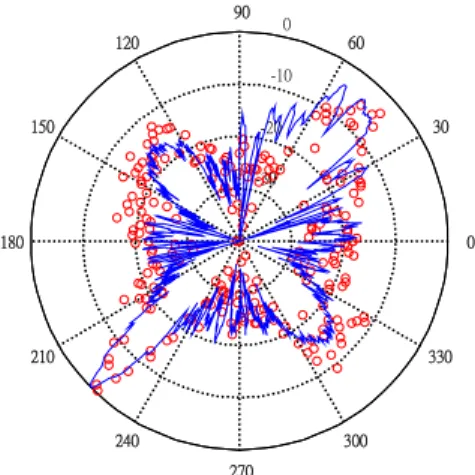
Two different placements of the scatterer are arranged to verify our model. First, the model is placed with its chassis facing the ground when the receiving antenna is pointing at the hood, and the transmitter is pointing at the left side of the vehicle body. In Fig.6, There are four peaks with roughly 90° interval between two adjacent peaks. These four peaks are contributed by the front panel of the hood, the back panel of the trunk, and the two side panels, respectively. Two of the peaks are about 8 dB above the others and about 180° apart. They are due to reflection from the left and right side panels, respectively. There is a difference of about 2 dB between the other two smaller peaks because the area of the front panel is about 1.24 times smaller than that of the back panel. 30 210 60 240 90 270 120 300 150 330 180 0 -30 -20 -10 0
Figure 6: Comparison of measured amplitude in the horizontal placement, - : measured, o :simulated.
Next, the vehicle model is turned over with the left side panel facing the ground. The receiving antenna is pointing at the hood when the transmitting antenna is pointing at the rooftop. The measured results are shown in Fig.7. There are four peaks with roughly 90 degree between two adjacent peaks. The four peaks are contributed by the front panel of the hood, the back panel of the trunk, the chassis, the roof top, the top of the hood and the top of the trunk, respectively. The highest peak is contributed by the scattering from the chassis and is 4 to 6 dB higher than the second group. The second highest group is larger than the other two but is also wider because it contains the scattering signals from more than one panel. The surface normal of the roof top and the top of the trunk are the same, and the surface normal of the top of the hood differs only slightly from those two. The
tops of the hood and the trunk are at the same horizontal level, and the roof top is about 5 cm higher. The scattering by these three panels appear closely but at slightly different rotation angles. The other two peaks are much wider than in the previous case. Because these two panels are of rectangular shapes having aspect ratio of 1:2.8 and 1:2.9, respectively, their shorter sides are rotated in the second case while the longer sides are rotated in the first case. Hence, the peaks are contributed by the same panels, but incurring different angular width.
-10 0 30 210 60 240 90 270 120 300 150 330 180 0 -30 -20
Figure 7: Comparison of measured amplitude in the vertical placement, - : measured, o :simulated.
Simulated and measured results of the two placements are shown in Figs.6 and 7, respectively. The four peaks match very well in both cases. The relative magnitudes of the peaks match well with the measurement, and their angular positions are only slightly different. From the simulation, it is discovered that the signal in the intervals between peaks is mainly contributed by the edge diffraction, and the magnitude deviation is on the order of 0.5 dB. In this part, the power level of the received signal shows fluctuation because of the scattering signal is contributed by more than one signal component. Again, the simulation and experiment results match reasonably well.
VI. CONCLUSION
In this work, we focus on the scattering analysis of vehicles. A process is developed with sophisticated combination to solve a complex problem. Since the closed form of the scattering field is used in the calculation, the total computation time is restricted to a tolerable level. The measurements and simulation results also match very well. Most features of the power distribution can be predicted in the program.
REFERENCES
[1] P. Blythe, "RFID for road tolling, road-use pricing and vehicle access control," IEE Colloq. RFID Technol., Oct. 1999.
[2] P. T. Blythe and P. J. Hills, "Road pricing in 5 cities: the ADEPT project," IEEE/IEE Conf . Veh. Navig. Info. Sys., pp.637-642, Oct. 1993.
[3] A. F. Dadds, "Microwave link for data communication between a moving vehicle and a roadside beacon." [4] Jakes, Microwave mobile communications, 1974
[5] J. B. Keller, ``Geometrical theory of diffraction,'' J. Opt.
Soc. Am., vol. 52, no. 2, pp. 116-130, 1962.
[6] R.G. Kouyoumjian, and P. H. Pathak, ``A uniform geometrical theory of diffraction for an edge in a perfectly conducting surface,'' IEEE Proc. vol. 62, no. 11, pp. 1448 - 1461, Nov. 1974.
[7] C. A. Balanis, Advanced Engineering Electromagetics, Wiley, 1989.
Dielectric-Resonator-Fed Active Horn
Antenna
Abstract — The main objective of this research is to
design and implement a DR-fed active rectangular horn antenna. A rectangular dielectric resonator of high permittivity with slot-coupling is used as the excitation of the waveguide to obtain broader impedance bandwidth, simple fabrication, and integration into planar circuit. A power amplifier with a gain of 10 dB is integrated into the horn antenna to enhance signal strength. Chokes are used to reduce the backward radiation level by about 8 dB.
Key Words — horn antenna, dielectric resonator,
active antenna.
I. INTRODUCTION
Horn antenna have been applied in satellite communications, radio links, direction-finding systems (DFS), cellular mobile communication, collision avoidance radar (CAR), and so on. Compared with other kinds of antennas like dipole, patch, spiral and slot antennas, horn antennas have the advantages including high gain, low VSWR and relatively wide bandwidth.
Recently, integration of active and passive components into to a planar circuit becomes more popular. Since the coaxial probe is a non-planar circuit and is difficult to integrate with other planar circuits. Several designs of transition from planar circuit to rectangular waveguide have been proposed, which can be categorized into microstrip-to-waveguide [1], stripline-to-waveguide [2], CPW-to-waveguide [3], [4], and so on. Typically, microstrip, stripline and CPW-to-waveguide transitions can be implemented with a transmission-line probe, aperture coupling, microstrip tapering, or a ridge waveguide. However, these feeding schemes may suffer from problems such as difficulty to integrate into planar circuit, difficulty to fabricate, high width-to-height ratio waveguide, and so on. In this work, a new coupling scheme of stripline-to-waveguide transition integrating dielectric resonator (DR) is proposed to improve the antenna characteristics.
To increase the antenna power, an amplifier circuit is integrated into the horn antenna. The design methodology, measured return losses, radiation patterns, and gain level of this DR-fed active horn antenna operating at 2.45 GHz are described.
Finally, chokes are added to reduce backward radiation. The field distribution of horn aperture in the E-plane does not vanish at the edge of the horn but diffuse around the edges to induce currents outside of the horn, which will increase the side-lobe level and backward radiation [5].
II. STRUCTURE OF DR-FED ACTIVE HORN ANTENNA
A. DR Design
Exact mathematical analysis on rectangular DR is quite difficult. However, approximate techniques have been proposed for analyzing rectangular DR. Dielectric waveguide model (DWM) is proposed to predict the
resonant frequency, impedance bandwidth, and radiation
Q, which have been verified by measurements [6]. The
equations are written as
2 2 2 tan 2 x x y z x k a k ⎛⎜ ⎞⎟= k +k −k ⎝ ⎠ (1) 2 2 2 0 x y z r
k
+
k
+
k
=
ε
k
2,
2
y zk
k
b
d
π
π
=
=
For a given resonant frequency f0 and DR parameters
r
ε
, a, and b as shown in Fig. 1, the wave number kx andthe value of a can be obtained from (1).
z
y x
a
d b
Figure 1 : An isolated rectangular DR.
If the dimensions of DR are chosen such that , the lowest three modes are TE
b
> >
d
a
111x, TE111zand TE111y, respectively. Fig. 2 shows the electric field
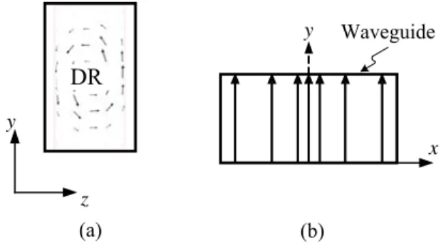
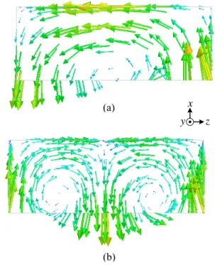
distributions on the y-z plane of the TEx mode of a rectangular DR. The field distribution looks like that generated by a magnetic dipole placed vertically at the center of DR. If the length b is relatively larger than the width d, the electric field distribution at
z
=
0, d
are nearly straight and parallel to the y-axis. The electric field distributions become similar to that of the TE10mode of a rectangular waveguide, rendering effective coupling to the TE10 waveguide mode.
z y y x (a) (b) Waveguide DR .
Figure 2 : E-field distributions: (a) TE111x mode of a
rectangular DR, (b) TE10 mode of waveguide.
B. Stripline-to-Waveguide Transition Design
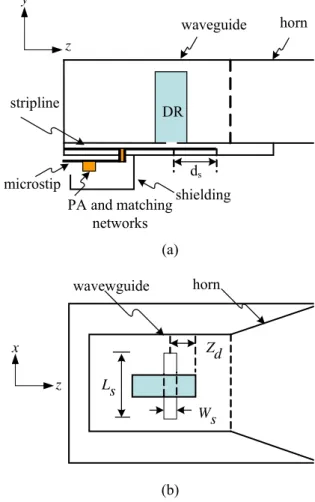
Fig. 3 shows the configuration of a DR-fed active horn antenna. An H-plane horn with an open bottom is fastened to the top ground plane of the stripline, and a rectangular DR is attached to the slot etching on the same ground plane to couple signals from the stripline to the waveguide efficiently.
The DR with relative permittivity of 18 is attached to the rectangular slot etched on the top ground plane of the stripline. The DR dimensions and relative permittivity of DR are chosen so that its lowest TE111x mode resonates at
2.45 GHz. The slot width should be narrow enough ( Ws<
λ/20) to prevent self resonance. Both the positions of DR and the length (Ls) of the slot can be adjusted to
obtain optimum coupling.
The side edges of the stripline substrate are enclosed by metal plates which are short-circuited to both ground planes to prevent fields from radiating into the air. The characteristic impedance of the stripline is 50 Ω. The open-stub of the stripline is about one-quarter of a guided wavelength at the operating frequency. In order to have the signal reflected from the waveguide back-wall to be in phase with the coupling field, the distance dw between
the wall and the DR is chosen to be about one-quarter guided wavelength of the waveguide. Under such conditions, the lowest TE111x mode of DR will be excited
and coupled to the TE10 waveguide mode. Note that by
the image theory, the equivalent height of the dielectric resonator is about twice the height of the physical resonator.
C. Active Element Design
The active element of the DR-fed active horn antenna is built by integrating a power amplifier (PA) into the antenna feedline of the passive horn antenna as shown in Fig. 3. The PA circuit with well input and output matching is placed on the bottom of the stripline to form a multilayered structure. A via is drilled from microstrip layer to stripline layer to connect the PA circuit and the horn antenna. The power matching scheme is applied in output matching to deliver maximum power.
D. Backward Radiation Reduction
Radiation pattern of horn antennas can be computed using presumed aperture distributions. In the H-plane, the field distribution of aperture is tapered to zero at the edges of horn. However, the field in the E-plane does not vanish at the edge of the horn, but diffuse around the edges to induce currents outside the horn to incur side lobes and back lobe. If currents on the outside edge can be reduced, the side-lobe level can be decreased, particularly in the backward direction of the horn.
To reduce the backward radiation of the horn antenna, chokes are placed at the edges of horn aperture with the opening of the chokes parallel to the horn aperture as shown in Fig. 4. While the depth of the chokes is adjusted to about one-quarter wavelength, the leakage currents are reduced and so is the backward radiation.
III.RESULTS
The H-plane horn is designed to have the maximum directivity of 6.2 dB at 2.45 GHz. The waveguide width and height are 40 and 80 mm, respectively. The width and the flaring angle of the horn are chosen to be 80 mm and 26.82°, respectively. The horn is fixed on the ground
plane with insulating screws, and the rectangular DR is
glued to the slot, which has a negligible effect on the operating frequency. The length and width of the slot are 23 and 2 mm, respectively, and the open stub is one-quarter guided wavelength, namely, d2=8 mm. The DR
has a relative permittivity of
ε
r=18, and dimensions of 36*24*9 mm3. The DR is placed on top of the center ofthe slot to achieve maximum coupling and can be moved waveguide stripline z y PA and matching networks microstip horn shielding DR Ls Ws Zd x z horn wavewguide (a) (b) ds
Figure 3: DR-fed active horn antenna: (a) side view, (b) top view.
(b) z y DR Horn Choke Choke 4 g λ (a) Choke x y
Figure 4: Configuration of DR-fed horn antenna with chokes: (a) side view, (b) front view.
along the y-direction for fine-tuning. It is observed that the measurement is insensitive to the precise positioning of the DR over the slot.
270 (a) 0 30 60 90 120 150 180 210 240 300 330 (b) 0 30 60 90 120 150 180 210 240 270 300 330
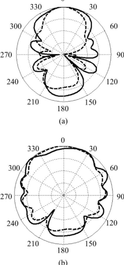
Figure 6 : Radiation patterns of DR-fed H-plane horn antenna at 2.45 GHz, 10 dB per division on radius, (Gmax=6.25 dBi), — : simulated co-polarized, --:
simulated cross-polarized, — × — : measured co-polarized, —o—: measured cross-co-polarized, (a) H-plane (b) E-H-plane.
If the dimensions of the slot are such that maxima coupling and the required resonant frequency are obtained, the positions of DR and the length of microstrip extending over the narrow slot can be regarded as coarse-
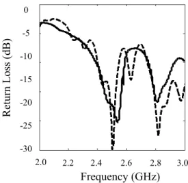
Fig. 5 shows that the simulated and measured return loss of the DR-fed horn antenna without amplifier. The small deviation is due to the tolerance of DR permittivity, the fabrication process and the connector used for the transition from coaxial to stripline. The calculated, simulated, and measured resonant frequencies of the DR are 2.45 GHz, 2.531 GHz and 2.51 GHz, respectively. The difference between simulated and measured results is 0.84 %. The beamwidth with a 10 dB return loss at 2.45 GHz is about 7.2 % by measurement and 8.0 % by simulation.
Fig. 6 shows the co-polarized and cross-polarized radiation patterns of the DR-fed horn antenna at 2.45 GHz in the E-plane (y-z plane) and H-plane (x-z plane), respectively. The simulated and measured co-polarized patterns agree well in both planes. In the H-plane, the co-polarized pattern shows a 10 dB beamwidth of 80° with the cross-polarized level lower than –20 dB in the main beam. The E-plane pattern is relatively broad due to the narrow horn aperture.
Fig. 7 shows the radiation patterns of horn antenna with or without chokes. Using the chokes reduces the antenna gain in the backward direction by about 7 dB. It is also found that the main-beam width is reduced.
Fig. 8 shows the radiation patterns of the DR-fed active horn antenna. The radiation patterns of the horn antenna with and without PA circuit are similar in both planes. However, the antenna gain with PA is increases by about 7.1 dB, which is the gain of the PA.
VI. CONCLUSION
DR-fed active horn antennas using DR for efficient coupling and integrating PA for gain enhancement are designed. This is the first demonstration of DR being used to excite a waveguide. A new feeding scheme is proposed which shows good characteristics, including better radiation pattern, wide impedance bandwidth and easy to integrate with planar circuit.
REFERENCES
[1] S.L. Romano and B. P. naranjo, “Ka-band waveguide-to-microstrip transition design and implementation,” IEEE AP-S Int. Symp., vol. 3, pp. 404, June 2002.
[2] B. N. Das and K. V. S. R. Prasad, “Excitation of waveguide by stripline- and microstrip-line-fed slots,” IEEE, Trans. Microwave Theory Tech., vol. 34, no. 3, Mar. 1986.
[3] Poly-grames research center, "Integrated transition of coplanar to rectangular waveguides,” IEEE
Microwave Symp. Dig., vol. 2, pp. 619-622, May
2001. 2.0 2.2 2.4 2.6 2.8 3.0 0 -5 -10 -15 -20 -25 -30 Frequency (GHz) Re turn L os s ( dB )
Figure 5 : Rreturn loss of DR-fed active horn antenna without amplifiers, — : simulation, -- : meaurement
[4] IMST, “A novel Coplanar transmission line to rectangular waveguide transition,” 1998.
[5] A. LaGrone and G. Roberts, “Minor lobe suppression in a rectangular horn antenna through the utilization of a high impedance choke flange,”IEEE Trans. Antennas Propagat., vol. 14, no. 1, pp. 102-104, Jan. 1966. 270 (a) 0 30 60 90 120 150 180 210 240 300 330 (b) 0 30 60 90 120 150 180 210 240 270 300 330
Figure 8 : Radiation patterns of the DR-fed H-plane horn antenna, —: with PA, --: without PA, (a) H-plane (Gmax =13.80 dBi) , (b) E-plane (Gmax =13.51
dBi). [6] R. K. Mongia and A. Ittipiboon, “Theoretical and
experimental investigations on rectangular dielectric resonator antennas,” IEEE Trans. Antennas
Propagat., vol. 45, no. 9, Sep. 1997.
90 (a) 0 330 300 270 240 210 180 150 120 60 30 (b) 0 330 300 270 240 210 180 150 120 90 60 30
Figure 7: Radiation patterns of DR-fed horn antenna at 2.45 GHz with or without chokes placed at the edges of horn, - -: with chokes, —: without chokes, (a) H-plane, (b) E-plane.
Dual-band Dielectric Resonator Antenna
Abstract — Dielectric resonator (DR) antennas haveattracted more attention due to its lack of conductor loss, and are very suitable for microwave and millimeter-wave applications. In this part, a dual-band dielectric resonator antenna is proposed. Probe feeding and aperture coupling mechanism are used to excite the
TE
101 and 102 modes of the DR antenna. With probe feeding, the resonant frequencies are 2.0 GHz and 2.8 GHz, and their 10 dB bandwidths are 5.8 % and 11.6 %, respectively. Measured and simulated results match reasonably well. With aperture coupling, additional resonant mode is introduced by the aperture. The bandwidth of theTE
101mode can be increased to 28 %. The characteristics of radiation patterns are also discussed.
y y
y
TE
Key Words —Dielectric resonator antenna, probe,
aperture coupling.
I. INTRODUCTION
Dielectric resonator made of low-loss and high-permittivity material has been widely used to implement microwave components. It is found that DR antennas are suitable for millimeter-wave applications because they are free of conductor loss. Unlike patch antenna, DR antennas can radiate from all surfaces, rendering high radiation efficiency and low Q-factor. Various radiation patterns can be obtained by exciting different modes of the dielectric resonator.
In [1], a DR attached on a circular slot and an eccentric ring slot is proposed to have dual-band operation. A grounded metal plate placed in a plane of symmetry of the electric field can reduce the sizes of DR antenna by half without perturbing the original field distribution.
In [2], a DR antenna with a coupling slot is proposed. The resonant frequencies of slot and DR can be merged to exhibit broadband characteristics. Both slot and DR antennas radiate as magnetic dipoles, rendering low cross polarization and similar radiation patterns.
Inverted-L and inverted-F antennas are compact with low profile and light weight. In [3], a rectangular DR with a grounded and inverted L-plate antenna is proposed. The DR serves both as a radiator and as a feed element to the L-plate.
III. RECTANGULAR DIELECTRIC RESONATOR ANTENNA
Analytical solution of electric field distribution in a dielectric resonator is complicated. A fast, simple and accurate approximation is required to predict the resonant frequency and field distribution of a dielectric resonator. In 1965, a simple approach that models the dielectric-air interface as a magnetic wall was proposed to predict the resonant frequencies of cylindrical resonators [4]. As the wave impinges from high-permittivity material upon low-permittivity material, the reflection coefficient approaches unity, which suggests that the interface can be modeled as a PMC wall.
Figs. 1 (a) and (b) show the simulated electric fields of and modes, respectively, in a rectangular dielectric resonator. The electric field is parallel to the
interface between the dielectric and the air. First, it is observed that the electric field is parallel to the interface, which complies with the approximation made in [4]. The electric fields spin around the walls of dielectric resonator, behaving as a transverse magnetic dipole. The
component of mode in the xy-plane is omni-directional, while that of the
TE
mode has a null in the y direction due to the antisymmetric pattern of electric fields. y 101TE
y 102TE
θE
TE
101y y 102 x y z (a) (b)Figure 1 : Electric field distribution in a rectangular dielectric resonator attached to the ground plane, (a) TE110 mode, (b) TE210 mode.
If a well is cut in a rectangular dielectric resonator to perturb the original electric field distribution of both modes, the electric field in the air will be enhanced as imposed by the boundary condition. The resonant frequencies are increased as well due to the lower effective dielectric constant. If the well is placed with an offset from the center of DR, the electric field of
TE
101mode is enhanced asymmetrically, as shown in Figure 2(b). Hence, the
E
θ component of theTE
102 mode on the xy-plane can be modified by tuning the geometry of the DR antenna.y y
II. ANTENNA CONFIGURATION
As shown in Fig.3, a rectangular dielectric resonator antenna with permittivity 20 and an offset well is mounted on a finite ground plane. The dimension of the dielectric resonator antenna is a × b × d, and that of the well is s1 × s2 × d. By observing the electric field
distribution in the DR antenna, a probe with length l1 is
attached on one side of the DR antenna to obtain good input impedance matching.
III. RESULTS AND DISCUSSIONS
Figure 3 shows the simulated and measured return loss, which agree reasonably well. The resonant frequencies of and modes are 2.0 GHz and 2.8 GHz, respectively. The associated 10 dB bandwidth of the mode is 5.8%, and that of the mode is 11.6%. y 101
TE
y 102TE
y 101TE
y 102TE
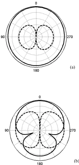
Figure 5 shows the simulated and measured radiation pattern of and mode on the H-plane. It is observed that the
E
θ component of both modes on theH-plane are nearly omnidirectional. However, the
cross-polarization of mode is higher than the co-polarization by 10 dB. Due to the image of electric field induced by the ground plane, the
E
θ component is significantly reduced in the x-direction. If the height of DR antenna is chosen to be quarter-wavelength of the mode, then the electric field in the well and itsimage due to the ground plane will interfere constructively in the x-direction.
y 101
TE
y 102TE
y 102TE
y 102TE
(a)Figure 3 : Return loss of probe-fed DR antenna as shown in Figure 4, εr = 20, a = 16 mm, b = 21 mm,
d = 40 mm, 2 rin = 1.3 mm, 2 rout = 4.5 mm, l = 16
mm, w1 =w2 = 4 mm, s1 = 10 mm, s2 = 13 mm, : simulation, - : measurement.
(b)
Figure 2 : Perturbed electric field distribution in a rectangular dielectric resonator attached on the ground plane, (a) TE110 mode, (b) TE210 mode.
Ly Lz a b d S1 S2 w2 w1 2rin 2rout z y (a)
Figure 4 : Configuration of probe-fed DR antenna with an offset well.
(b)
Figure 5 : Measured radiation pattern of probe-fed dielectric resonator antenna, (a)
TE
mode, (b) mode, all parameters are the same as in Fi y 101 y 102TE
gure 3. solid line:
E
θ , dashed line :E
φFigure 6 shows an aperture-coupled DR antenna. The power is coupled to the antenna through an aperture. By tuning the width wa of the aperture and the length of
can be achieved. A shorted metal plate is used to terminate the electric field to reduce the length of DR antenna. The aperture also introduces additional resonant mode. The resonant frequency of the aperture is determined by its length La. By properly designing the
length of aperture, its resonant frequency can be tuned toward that of mode and thus widen the bandwidth as shown in Fig.7. The height of DR is chosen close to quarter-wavelength of the mode. Hence, the θ component of mode on the xy-plane can be improved, as shown in Figure 8. The resonant frequencies of mode and the aperture are 1.529 GHz and 1.68 GHz, respectively, which are merged to form a wider bandwidth of 28%. The upper band is contributed by the mode with resonant frequency of 2.4625 GHz and 10 dB bandwidth of about 2%. The radiation patterns are shown in Figure 8.
y 101
TE
y 102TE
E
TE
102y y 101TE
y 102TE
t Wg z x y Lg b a d s2 s1 microstip line aperture ground plane metal plateBy using aperture coupling mechanism, the separation of feeding network and radiator can surpress supurious radiation, and the antenna module is easy to integrate with other planar circuits.
VI. CONCLUSION
In this work, a dual-band DR antenna is proposed. Probe and aperture coupling are used to feed the DR antenna, and good impedance matching can be obtained. With probe feed, the resonant frequencies are 2.0 GHz and 2.8 GHz, and their associated 10 dB bandwidths are 5.8 % and 11.6 %, respectively. Measured and simulated results match reasonably well. The length of DR antenna can be reduced by inserting a shorted metal plate. Aperture-coupling mechanism can be used to feed the antenna and introduce additional resonant mode. By proper design of the aperture size, the bandwidth of DR antenna can be increased. The radiation pattern can be improved by choosing the height of the DR antenna to be quarter-wavelength of the operating frequency.
REFERENCES
[1] T. A. Denidni and Q. Rao, “Hybrid dielectric resonator antennas with radiating slot for dual-frequency operation," IEEE Antennas Wireless
Propagat. Lett., vol. 3, pp. 321-323, 2004.
[2] A. Buerkle, K. Sarabandi, and H. Mosallaei, “Compact slot and dielectric resonator antenna with dual-resonance, broadband characteristics," IEEE
Trans. Antennas Propagat., vol. 53, no. 3, pp.
1020-1027, Mar. 2005.
[3] K. Lan, S. K. Chaudhuri, and S. S. Naeini “Desing and analysis of a combination antenna with rectangular dielectric resonator and inverted L-plate," IEEE Trans. Antennas Propagat., vol. 53, no. 1, pp. 495-501, Jan. 2005.
[4] H. Y. Yee, “Natural resonant frequencies of microwave dielectric resonators," IEEE Trans.
Microwave Theory Tech., vol. 13, pp. 256-258, Mar.
1965. wa La Ls wm aperture dielectric resonator s1 s2 a microstrip line metal plate b Lg Wg ds
Figure 6 : Configuration of aperture-coupled DR antenna.
Figure 7 : Simulated return loss of aperture-coupled DR antenna, a = 10 mm, b = 39 mm, d = 24 mm, s1 = 12 mm, s2 = 8 mm, La = 24 mm, wa=
5 mm, ds = 16 mm, wm = 1.15 mm, Ls=6.5 mm, t =
(a)
(b)
Figure 8 : Simulated radiation pattern on the
H-plane, (a) 1.529 GHz, (b) 2.4625 GHz, all
parameters are the same as in Figure 7, solid line: