Labeling Points on a Single Line
∗
Yu-Shin Chen, D.T. Lee
†, and Chung-Shou Liao
‡Institute of Information Science
Academia Sinica Nankang, Taipei, Taiwan
Email: [email protected]
[email protected]
[email protected]
November 30, 2004
Abstract
In this paper, we consider a map labeling problem where the points to be labeled are restricted on a line. It is known that the 1d-4P and the 1d-4S unit-square label placement problem and the Slope-4P unit-square label placement problem can both be solved in linear time and the Slope-4S unit-square label placement problem can be solved in quadratic time in [7]. We extend the result to the following label placement problem: Slope-4P unit-height (width) label placement problem and elastic labels and present a linear time algorithm for it provided that the input points are given sorted. We further show that if the points are not sorted, the label placement problems have a lower bound of Ω(n log n), where n is the input size, under the algebraic computation tree model. Optimization versions of these point labeling problems are also considered.
1
Introduction
When drawing a map, in order to let people know what is on the map, the main approach is attaching texts or labels to geographic features on the map. How to place labels so that they do not overlap, is a well-known important problem in cartography. Thus, there are
∗Supported in part by the National Science Council under Grants NSC-92-2213-E-001-024,
NSC-93-2213-E-001-013, NSC-93-2422-H-001-0001, and NSC-93-2752-E-002-005-PAE.
†Also with the Dept. of Computer Science and Information Engineering, National Taiwan University.
Email:[email protected]
many research results on this topic and many algorithms have been developed for labeling points that are on lines [7, 8, 9, 15] or in a region [5, 6, 10, 11, 12, 14, 17, 19]. In the ACM Computational Geometry Impact Task Force report [2] the map label placement is listed as an important research area.
Let S denote a set of points S = {p1, p2, . . . , pn} in the plane, called anchors.
Asso-ciated with each anchor there is an axis-parallel rectangle, called label. The point-feature
label placement problem or simply point labeling problem, is to determine a placement of
these labels such that the anchors coincide with one of the corners of their associated labels and no two labels overlap. The point labeling problem for labeling an arbitrary set of points has been shown to be NP-complete [6, 10, 11, 14], and some heuristic algorithms were presented in [4, 6, 19].
There are many variations of the point labeling problem, including shapes of the labels, locations of the anchors to be labeled and where the labels are placed. Three common shapes of the labels considered were circles, squares and rectangles. Sometimes, the rectangular labels may be given additional constraints, e.g., the width and height may satisfy a certain aspect ratio. The placement of the labels may be restricted. For instance, the anchors must be on the corners of the labels (i.e., fixed-position model), or on the boundary of the label (i.e., sliding model). One may also consider an optimization version of the problem, e.g., maximizing the size of labels.
Strijk and Wolff [17] showed that to decide if a set of points can be labeled with unit circles is NP-hard, and also that there is a constant 0 < δ < 1 such that it is NP-hard to label points with uniform circles of diameter greater than δ · dopt, where dopt denotes the
optimal diameter. They presented an approximation algorithm for labeling points with uniform circles whose diameter is about 1/19.59 times the optimal in O(n log n) time [17]. The elastic point labeling problem, is yet another variation, and is defined as follows: Given a set of n points on the plane, each of which is associated with an elastic rectangular label of a given area, we want to choose a valid height (or width) for each label and a corner to place at its associated anchor so that no two labels overlap. A label is said to be elastic if its width and height can vary but its area remains a constant.
which the anchors must be at the corners of the labels is NP-hard. They considered the elastic point labeling problem when n anchors lie on the x-axis and m anchors lie on the
y-axis, and the labels for the anchors on the x-axis (resp. y-axis) have an edge coincident
with the x-axis (resp. y-axis) lying in the same quadrant [8] and presented an O(nm) algorithm. They also considered the rectangle perimeter point labeling problem [9], in which the given elastic labels are to be placed on anchors that lie on the boundary of a given rectangular map. They combined the solution of the axis case and the two-parallel-line case to solve the rectangle perimeter point labeling problem in O(n4) time,
where n is the number of anchors. The two-parallel-line case is similar to the two-axis case except that the points to be labeled lie on two parallel lines.
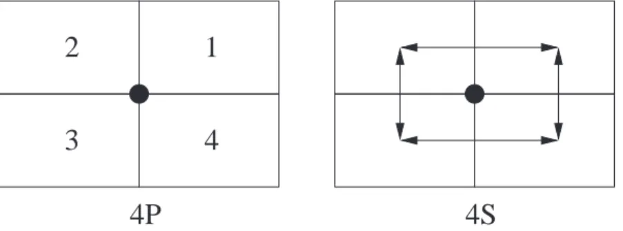
In this paper we consider the case when the anchors lie on a line and are to be labeled with rectangular labels. We consider two main models. One is fixed-position model, denoted 4P model, in which a label must be placed so that the anchor coincides with one of its four corners, and the other is sliding model, denoted 4S model, in which a label can be placed so that the anchor lies on one of the four boundary edges of the label. Figure 1 shows these two point labeling models, among others, that have been studied previously [12, 15]. The positions {1, 2, 3, 4} in 4P model shown in Figure 1 denote the corner positions of labels coincident with the anchor, and the arrows in 4S model indicate the directions along which the label can slide, maintaining contact with the anchor.
4S
1
4
4P
2
3
Figure 1: Illustration of 4P and 4S models.
Extending the result of [7], we consider the problem of labeling points on a sloping line with rectangular labels of unit-height (or unit-width) in 4P model, referred to as
Slope-4P unit-height label placement problem and the problem of maximizing the size of
bottom edge coincide with the line in 4S model, referred to as 1d-4S equal-width label
maximization problem. We also address the elastic point labeling problem, where points
to be labeled lie on a sloping line.
This paper is organized as follows. In Section 2, we give some definitions and notation about our point labeling problems. In Section 3, we consider the Slope-4P unit-height label placement problem for points lying on a sloping line. In Section 4, we extend the result of Section 3 to the case where the labels are elastic. In Section 5, we consider the 1d-4S equal-width label maximization problem, and give a lower bound of the time complexity of the 1d-4S equal-width label placement (decision) problem.
2
Preliminaries
In this section, we introduce some terminology and notation. Consider a set P =
{p1, . . . , pn} of n anchors on a line L such that they are sorted in ascending x-coordinate,
i.e., pi.x < pi+1.x, i = 1, 2, . . . , n − 1, and for each pi, there is an axis-parallel rectangular
label li.
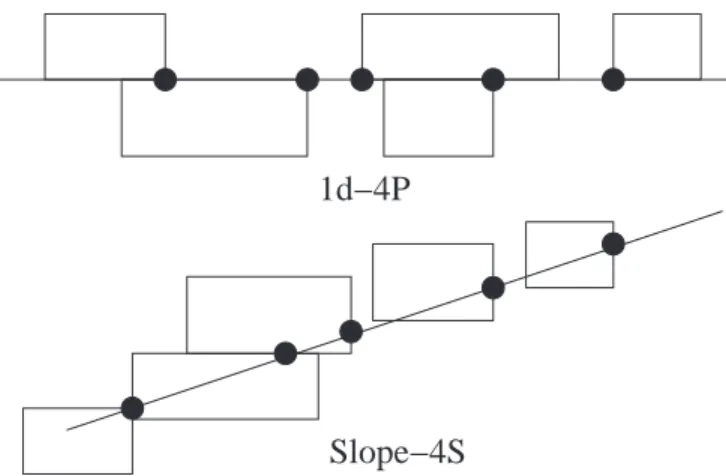
We shall use prefixes, 1d- or Slope- to refer to the problems in which the anchors lie on a horizontal or a sloping line, respectively. Combined with 4P and 4S model as described previously, we have, for example, 1d-4P denotes that the anchors lie on a horizontal line and each label has four possible placement positions, and Slope-4S denotes that the anchors lie on a sloping line and each anchor can lie on any of the four boundary edges of a label.
1d−4P
Slope−4S
A k-tuple Rk = (r1, · · · , rk) is a k-realization of labels l1, l2, . . . , lk for P such that each
ri encodes a position of li. If no two labels in Rk intersect each other, Rk is said to be
a good k-realization. Our goal is to find a good n-realization Rn, or good realization for
short, for a given P . See, for example, Figure 2 for a good 5-realization in 1d-4P and Slope-4S models.
A point u is said to be above another point v, or v is said to be below u if the y-coordinate of v, v.y, is smaller than that of u, u.y, i.e., v.y < u.y . A point u is said to be below, on and above a line L, if the y-coordinate of u is smaller than, equal to, and greater than, respectively, the y-coordinate of the vertical projection point uL of u on L.
Let δ denote the length of the unit for the unit-height label placement problem discussed in this paper such that each anchor has a rectangular label of the same height δ > 0.
3
Labeling Points on a Sloping Line with Unit-Height
Labels
Garrido et al. solved the Slope-4P unit-square label placement problem in O(n) time, and the Slope-4S unit-square label placement problem in O(n2) time [7]. They made use
of a concept, called shadow, which is determined by the last two labels. For our Slope-4P unit-height label placement problem this concept unfortunately does not work. Figure 3 shows that the shadow of the realization R = {r1, r2, r3, r4} defined by the last two labels
as stated in Lemma 4 in [7] will produce an incorrect labeling for the next label at p5. We
therefore propose a new idea, called top and bottom domination labels, for the Slope-4P unit-height label placement problem. It is obvious that the case for unit-width labels is similar, so we consider only the case for unit-height labels. We assume that the slope of the line is positive without loss of generality.
Definition 3.1 In a realization R, a label li is called a top label, if its upper-right corner
qi is above the sloping line, and a bottom label, if qi is below or on the sloping line.
Definition 3.2 In a good realization R, the feasible region, denoted F (li), of each label li
with respect to label lj, for all j > i, or simply the feasible region of each label li, is defined
r
1p
5r
3r
4r
2Figure 3: An illustration of how the notion of shadow of the realization R = {r1, r2, r3, r4}
as stated in [7] is not adequate to determine the placement of the fifth label.
if li is a bottom label, F (li) is the intersection of NDqi and Abi, where NDqi is the locus of
points not dominated 1 by the upper-right corner q
i of li and Abi is the region containing
points whose y-coordinates are no less than the y-coordinate of the bottom boundary edge of li; if li is a top label, F (li) is the intersection of NDqi and Ati , where NDqi is defined
as above, and Ati is the region containing points whose y-coordinates are no less than the
y-coordinate minus δ of the bottom boundary edge of li.
Definition 3.3 In a good realization R, label lj is said to cover label li or label li is covered
by label lj, for j > i, if F (lj) ⊆ F (li). That is, whenever label lk can be placed in F (lj) it
can be placed in F (li) for i < j < k (see Figure 4).
li
lj
Figure 4: Label lj covers li
Definition 3.4 In a good realization R, the last top label, is called the top domination label, denoted dt, and the last bottom label, the bottom domination label, denoted db.
Lemma 3.5 The pair of labels dt and db covers all other labels in any good realization.
1A point u is said to dominate another point v, or v is said to be dominated by u, if both x- and y-coordinates of v are no greater than those of u.
Proof: For an arbitrary good realization R, the feasible region F (li) of each top label li
contains the feasible region F (dt) of dtobviously. So dtcovers all the top labels. Similarly,
since F (db) ⊆ F (lj) for each bottom label lj, db covers all the bottom labels. The lemma
follows. 2
Let the top and bottom domination labels associated with a good k-realization Rk be
denoted dtk and dbk respectively.
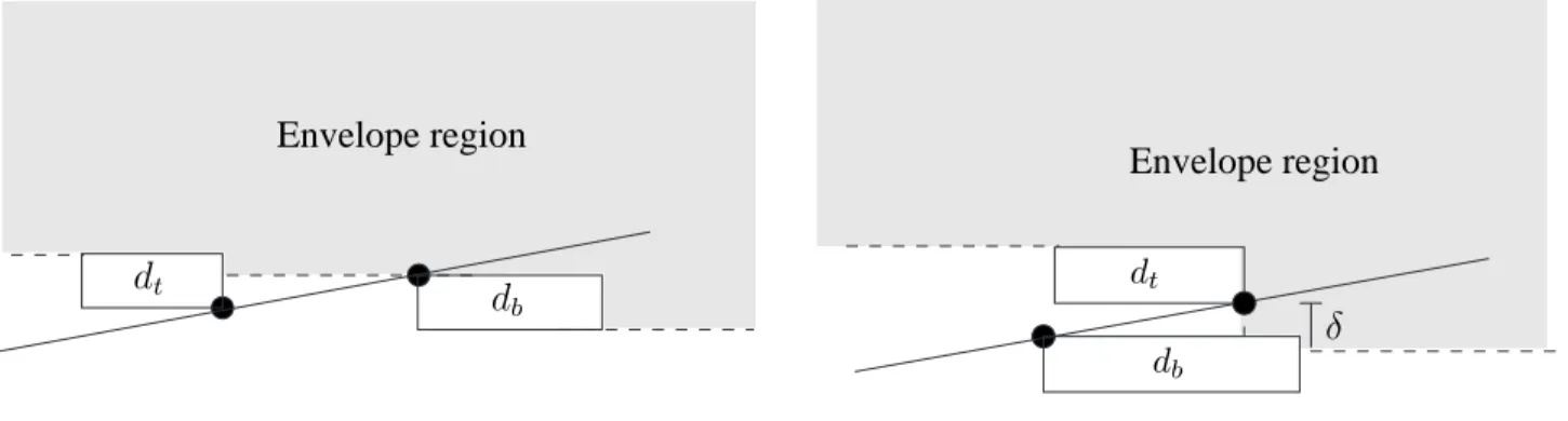
Definition 3.6 For a good k-realization Rk, we define its associated envelope region
Ek as the intersection of F (dbk) and F (dtk) (see Figure 5). Given two k-realizations,
R1
k, and R2k, we say that the domination pair d1bk and d
1
tk associated with R
1
k, covers
the domination pair d2
bk and d
2
tk associated with R
2
k, if the envelope region Ek2 contains
the envelope region E1
k, i.e., Ek1 ⊆ Ek2. Two k-realizations Rk1, and R2k are said to be
comparable if E1
k ⊆ Ek2 or if Ek2 ⊆ Ek1. Otherwise, they are said to be incomparable.
Envelope region Envelope region dt d b dt db δ
Figure 5: The envelope region.
Lemma 3.5 plays an important role for Slope-4P model and it implies that if a new label lk+1 is added to a k-realization Rk, we only need to check if label lk+1 can be placed
to lie totally in the envelope region associated with Rk, and if so, which positions lk+1 can
be placed so as to obtain a good (k + 1)-realization Rk+1.
Therefore, we will simply use the ordered pair (dbk, dtk) of bottom and top domination labels of Rk to represent the k-realization, as it defines the envelope region Ek associated
with Rk.
For convenience, we shall encode the label positions in a k-realization, using elements in {1, 2, 3, 4}, as described in Figure 1. That is, Rk = {r1, r2, . . . , rk} is a k-realization,
It turns out that given a k-realization Rk, there are six cases of possible positions that
lk+1 can be placed as follows.
1. rk+1∈ {1, 2, 3, 4}. 2. rk+1∈ {1, 2, 4}. 3. rk+1∈ {1, 4}. 4. rk+1∈ {1, 2}. 5. rk+1∈ {1}. 6. rk+1= ∅.
And the notion of envelope given in Definition 3.6 simplifies our algorithm. We shall adopt an incremental algorithm by placing labels one at a time in ascending order of the
x-coordinates of the anchors on the sloping line. The algorithm is greedy in nature. That
is, when we consider adding the next label, lk+1 to a k-realization Rk, if we have more
than one choice to put the label, we shall place it so that the resulting envelope associated with the new (k + 1)-realization is as maximal as possible, as will be shown below. Thus, we adopt the following maximal placement strategy.
1. If rk+1 ∈ {1, 2, 3, 4}, we let rk+1 = 3.
2. If rk+1 ∈ {1, 2, 4}, we let rk+1 = 2 or rk+1 = 4, as the resulting realizations may be
incomparable.
3. If rk+1 ∈ {1, 4}, we let rk+1 = 4.
4. If rk+1 ∈ {1, 2}, we let rk+1 = 2.
5. rk+1∈ {1}.
6. rk+1= ∅.
Lemma 3.7 For anchors {p1, p2, . . . , pi}, there are at most two incomparable i-realizations.
Proof. We prove it by induction on label index i. For i = 1 and i = 2, this lemma holds trivially. Suppose that the induction hypothesis holds for i = k. Consider i = k + 1. By induction hypothesis, there are at most two k-realizations R1
k and R2k. Let (djbk, d
j tk) represent the bottom and top domination labels associated with Rkj respectively, j = 1, 2. For each of the two k-realization Rk, there are at most two feasible position choices for
rk+1 at the same time according to the maximal placement strategy mentioned above.
Note that rk+1 can be either dbk+1 or dtk+1 in Rk+1. Thus, the following are the four (k + 1)-realizations: (rk+1, d1tk) represents R 1b k+1, (d1bk, rk+1) represents R 1t k+1, (rk+1, d2tk) represents R2b k+1 and (d2bk, rk+1) represents R 2t
k+1. We distinguish the following cases to
show that there are actually at most two incomparable (k + 1)-realizations.
Case 1: Assume rk+1 = 3 (when rk+1 ∈ {1, 2, 3, 4}) for one of R1kand R2k, say R1k without
loss of generality. In this case, we have at most three possible realizations: R1b k+1,
R2b
k+1, and R2tk+1. Since Ek+12t ⊆ Ek+11b , we have at most two (k + 1)-realizations R1bk+1
and R2b k+1.
Case 2: Assume rk+1 = 4 (when rk+1 ∈ {1, 4}) for one of R1k and R2k, say R1k without
loss of generality. There are three realizations: R1b
k+1, R2bk+1, and R2tk+1.
Subcase 2-1: If rk+1 = 2 or 4, that is, rk+1 ∈ {1, 2, 4} for R2k, then obviously R1bk+1
and R2b
k+1 are comparable, and one can be eliminated.
Subcase 2-2: If rk+1 ∈ {1, 4} for R2k, no R2tk+1 exists. (The subcase rk+1 ∈ {1, 2}
is similar.)
Subcase 2-3: If rk+1 = 1 for Rk2, then either Ek+12b ⊆ Ek+11b (as rk+1 = db) or
E2t
k+1 ⊆ Ek+11b (as rk+1 = dt) and hence one can be eliminated.
Case 3: Assume rk+1 = 2 (when rk+1 ∈ {1, 2}) for one of R1k and R2k, say R1k without
loss of generality. There are three realizations: R1t
k+1, R2bk+1, and R2tk+1.
Subcase 3-1: If rk+1 = 2 or rk+1 = 4, that is, rk+1 ∈ {1, 2, 4} for R2k, then since
rk+1 = 4 is feasible for R2k, Ek+11t ⊆ Ek+12t .
Subcase 3-2: If rk+1 ∈ {1, 2} for R2k, no R2bk+1 exists. (The subcase rk+1 = 1 is
Case 4: Assume rk+1 = 1 for one of R1k and R2k, say R1k without loss of generality. There
are three realizations: R1b
k+1, R2bk+1, and R2tk+1, if rk+1 = db, and R1tk+1, R2bk+1, and
R2t
k+1, if rk+1 = dt.
Subcase 4-1: If rk+1 = 2 or rk+1 = 4, that is, rk+1 ∈ {1, 2, 4} for R2k, then Ek+11b ⊆
E2b
k+1, Ek+12t if rk+1 = db. (As rk+1 = dt, it’s similar.)
Subcase 4-2: If rk+1 = 1 for Rk2, no R2tk+1 exists as rk+1 = db. (As rk+1 = dt, it’s
similar.)
Case 5: Assume rk+1 ∈ {1, 2, 4} for R1k and rk+1 ∈ {1, 2, 4} for R2k, there are four
real-izations: R1b
k+1, R1tk+1, R2bk+1, and Rk+12t . Since rk+1 = 4 is feasible for both Rk1 and
R2
k, so R1tk+1 = R2tk+1. For both R1bk+1 and R2bk+1, rk+1 = 4. So they are comparable
and one can be eliminated.
Case 6: Assume rk+1 = ∅ for one of R1k and R2k, it’s trivial.
For every case, there are at most two incomparable (k + 1)-realizations. 2
We thus have immediately the following algorithm, Algorithm Slope-4P, for finding a good realization for the Slope-4P unit-height label placement problem, using an iterative method by considering the labels one at a time in order.
Algorithm Slope-4P.
Input: A sloping line L with positive slope, a set of anchors P = {p1, p2, . . . , pn} on
L sorted in ascending x-coordinate, and the corresponding label width l1, l2, . . . , ln (the
heights of all the labels are identical, denoted δ ).
Output: A good realization R of P if it exists, and nil otherwise. Method.
1. Assume that we maintain at most two realizations R1, R2 for the set P of anchors
and let their associated bottom and top domination labels be (d1
b, d1t), (d2b, d2t)
re-spectively.
2. Let P1, P2 denote the set (⊆ {1, 2, 3, 4}) of positions the next (new) label can be
3. We consider the anchors in ascending order of their x-coordinates one at a time;
4. R1, R2, P1, P2 ← ∅ and d1
b, d1t, d2b, d2t ← nil;
5. For each realization Rj, j = 1, 2, we keep two temporary realizations, Rj b, and Rj t;
6. For i = 1 to n
Determine Pj with respect to (dj
b, djt), for ri, j = 1, 2;
If (P1 = ∅ and P2 = ∅) then return nil and break;
Temporarily store possible realizations in Rj b, Rj t for Pj, j = 1, 2,
according to the maximal placement strategy;
Compare R1 b, R1 t, R2 b, R2 t to get at most two maximal realizations;
Update Rj from the previous step, and also update (dj
b, djt), for j = 1, 2;
END;
Theorem 3.8 The Slope-4P unit-height (width) label placement problem can be solved in linear time when the input anchors are given sorted.
Proof. By Lemma 3.7 there are at most two incomparable realizations that need to be maintained at each step, and the envelope regions of these two realizations are maximal. Thus, the algorithm Slope-4P is able to find at least one good realization for the input anchor set P , if there exist feasible solutions.
As we determine the possible label positions of the next label, only two realizations (d1 b,
d1
t), (d2b, d2t) of bottom and top domination labels have to be checked according to previous
lemma. It takes constant time in each iteration. Therefore the total time complexity of
Algorithm Slope-4P is O(n). 2
4
Labeling Points on a Sloping Line with Elastic
La-bels
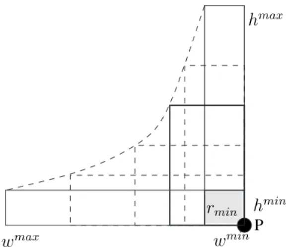
We now consider the case when the labels are elastic. An elastic rectangle E is a family of rectangles specified by a triplet (α, H, W ), where α is the area of any rectangle in
the range of the width. Given an anchor p, the placement of an elastic label E will be specified by (p, Q)(E), where Q ⊆ {1, 2, 3, 4} is a set of possible label position indexes and the anchor p is to coincide with a corner of a rectangle in E. The position index is the same as in the 4P model defined previously. Note that given a label position p(E), the family E of rectangles is described by a hyperbolic segment tracing out the locus of the corner of the elastic rectangle opposite to p. In our model, we assume hmin and wmin
are both set to be unity. Figure 6 shows an elastic rectangle with Q(E) = {2}, and the hyperbola shown as a dashed curve. The notation rmin denotes the unit rectangle of
height hmin and width wmin.
P hmin wmin hmax rmin wmax
Figure 6: An instance of an elastic rectangle
Theorem 4.1 For a set of anchors, the Slope-4P elastic label model has a good realiza-tion if and only if Slope-4P unit-width label model (slope is less than or equal to hmin
wmin
or Slope-4P unit-height label model (slope is greater than or equal to hmin
wmin ) has a good
realization.
Proof. If there exists a good realization for Slope-4P unit-width (respectively height) label placement problem instance, then this solution is a solution to the Slope-4P elastic label placement problem in which width w = δ (respectively height h = δ), and height
h = α/δ (respectively width w = α/δ). Conversely, suppose there exists a good realization Re for Slope-4P elastic label placement problem instance. Let us consider the case when
the slope of the sloping line is less than or equal to hmin
is greater than or equal to hmin
wmin is similar. We claim that we can let all elastic labels be unit-width labels, where the unit width δ is set to be wmin and obtain a good realization.
First, it is obvious that there exists a good realization R0 for Slope-4P unit-rectangle r min
label model for the input instance by reducing each label in Re to rmin. Next, we let each
top label in R0 grow upwards to be of height h = α/wmin. Similarly, we let each bottom
label in R0 grow downward to be of height h = α/wmin. Since the slope of the sloping line
is less than or equal to hmin
wmin, there is no intersection for every label of width w = wmin and height h = α/wmin. Then we have a good realization for Slope-4P unit-width label
placement problem, where δ = wmin. 2
5
Maximizing Label Sizes and the Lower Bound
5.1
Maximizing Label Size for Slope-4P Unit-height Model
The maximization version of Slope-4P unit-height label model (Slope-4P unit-width la-bel model, similarly) is defined as follows: Given a set of n anchors P = {p1(x1, y1),
p2(x2, y2), . . . , pn(xn, yn)} on a sloping line with positive slope, where (xi, yi) are the
x-and y-coordinates of anchor pi, i = 1, 2, . . . , n, and each anchor pi is associated with a
rectangular label of unit height h = δ and width li, find the maximum stretch factor λmax
such that the width and height of each label are multiplied by λmax for which there exists
a good realization. For this maximization problem, we can use an idea similar to that used in [7] to solve this problem and the following result immediately follows.
Theorem 5.1 The maximization version of Slope-4P unit-height (width) label placement problem can be solved in time O(n2log n).
5.2
Maximizing Label Size for 1d-4S Equal-width Model
The maximization version of 1d-4S equal-width label placement problem is defined as follows: given a set P = {p1, p2, . . . , pn} of n anchors on a horizontal line, find the
maximum label width wmax such that there is a good realization of P . We show below
that this problem can be solved in O(n2) time instead. We use an iterative approach to
method and obtain an alternating good realization in a greedy manner [3] for the 1d-4S equal-width label placement problem in linear time, assuming the input anchors are given sorted. That is, we place labels as left as possible for each anchor, and alternately place labels above and below the line in sorted order. 2 Therefore, we can separate the point
set P into two parts, Po= {pi | i is odd } and Pe = {pi | i is even }. The labels of Po are
placed above the line and the labels of Pe are placed below the line. The solutions wmaxo
and wmax
e of Po and Pe, respectively can be computed independently and the smaller of
wmax
o and wemax is the solution. We shall consider only the problem of Po and the other
problem is similar. This problem is equivalent to finding an interval of maximum length for each anchor in Po such that each interval is of equal length, and there is exactly one
anchor in each interval. In other words, we would like to place cuts on the horizontal line to form a collection of equal-length cut intervals, each containing exactly one anchor.
We would proceed by processing these anchors in Po one at a time from left to right
and placing cuts in an appropriate manner. Assume that these anchors are ordered from left to right as pi, i = 1, 2, . . . , m. Let xi denote the x-coordinate of the ith anchor and ci
denote the x-coordinate of ith cut. We use (xm − xj)/(m − j − 1) to be the (weighted)
cut interval length, denoted X. Initially j = 1, clearly the first cut can be placed at the leftmost point, thus c1 = x1. Note that X is an upper bound on the optimal label
width. We then proceed to place cut ci which is at distance X to the right of cut ci−1 for
i ≥ 2, until either there is more than one anchor in the cut interval or there is no anchor
in the cut interval. When either case occurs, we need to adjust the cut interval length
X. For each anchor pi, we maintain a safety clearance sci = |ci− xi|, weighted clearance
wcj = scj/(j − 1), j ≥ 2, and an invariant condition that there is exactly one anchor in
each cut interval.
Case 1: Suppose there is no anchor in the cut interval or cut i happens to be placed at the ith anchor, i.e. ci = xi.
In this case we can separate the rest of anchors from what we have processed, and treat the remaining set of anchors as a new subproblem. In the former case we will search for the next anchor pj, rename it p1, place a cut c1 at it and update X = (xm−xj)/(m−j −1).
2It is shown in [3] that one can always obtain an alternate label placement, if there is a feasible solution
While in the latter case, anchor pi would play the role of p1 and cut ci would play the
role of c1, and this process continues.
Case 2: Suppose there is more than one anchor in the cut interval.
Assume that this happens for cut ck+1and that the distance between cut ckand the second
anchor pk+2 to its right is Y , Y < X. This means that the label width X is too large and
we need to re-adjust the length of cut interval. We first calculate the new cut interval length X0 = [(k −1)X +Y ]/k which is strictly less than X. Let D = X −X0. Let U be the
minimum weighted clearance, i.e., U = min{wcj | 2 ≤ j ≤ k}. If D < U , then we have
a new arrangement of cuts and the invariant condition that each cut interval has exactly one point is maintained. We then update the weighted clearances for all the anchors by decrementing each wcj by D, place cut ck+1 at anchor pk+2, let sck+1 = |ck+1 − pk+1|,
wck+1 = sck+1/k and continue the processing using X0 as the new cut interval length with
pk+2 being the next anchor to be considered when placing next cut ck+2. Otherwise, i.e.,
D ≥ U, assume that the minimum weighted clearance wcj0(= U) occurs at pj0. We know that if we select the cut interval length as Xwc = X − wcj0, then cut cj0 will be placed at
pj0, and there is exactly one anchor in each cut interval among p1 to pj0. The invariant condition (there is exactly one anchor in each cut interval) is maintained among p1 to pj0 if we use Xwc to be the cut interval length. We can then separate the rest of anchors from
pj0 on to be a new subproblem such that the anchor pj0 and cut cj0 would play the role of p1 and c1 respectively, and the process repeats by using the cut interval length Xwc.
Note that if there exists more than one weighted clearance wcj0 which equals U, we pick the rightmost anchor pj with the largest index j.
In Case 2 we need at most O(n) time to proceed to a cut interval containing more than one anchor, and recompute a new cut interval width, resulting in a new subproblem. Since there are at most O(n) subproblems, the total time complexity is O(n2). We need
O(n) space to maintain the information of anchors, cuts and weighted clearances. We
therefore conclude with the following theorem.
Theorem 5.2 The maximization version of 1d-4S equal-width label placement problem can be solved in O(n2) time and O(n) space.
5.3
The Lower Bound
Now we consider the lower bound for the 1d-4S equal-width label placement problem. It is known that when the points are given sorted, the problem can be solved in linear time [3, 7]. We show that the problem requires Ω(n log n) time, if the points are arbitrary. We adopt the algebraic computation model of Ben-Or [1] in which we have a random access machine with real arithmetic, and each arithmetic operation takes constant time. Consider the following decision version of the 1d-4S equal-width label placement problem.
1d-4S equal-width label placement decision problem
Instance: Given a set P = {p1, p2, . . . , pn} of n points on the real line and a width w.
Output: Yes, if there exists a disjoint set of n intervals, each of width w such that each interval contains exactly one point, and these intervals may have their endpoints common to each other, and no, otherwise.
We shall prove the lower bound of the above 1d-4S equal-width label decision problem by problem reduction [16]. Specifically we shall reduce to it the uniform gap problem, a well-known problem with an Ω(n log n) lower bound, where n is the input size [13]. The uniform gap problem is described in the following:
Instance: Given a set of n real numbers X = {x1, x2, ..., xn} and a real number ² ≥ 0.
Output: Yes, if the gaps between consecutive numbers are uniformly equal to ² (Two numbers xi and xj are said to be consecutive if xi ≤ xj and there exists no other number
xk such that xi < xk< xj.); No, otherwise.
The problem reduction is as follows. Consider an instance X = {x1, x2, ..., xn}. Assume
x1 is the minimum of X and xn is the maximum. We must have xn− x1 = (n − 1)²; else,
return No obviously. Let w = ² and assign p1 = x1, pn = xn − ². We shall construct
two equal-width label placement problem instances I and I0. Let the instance I with
pi = xi− ², for each pi, 1 < i < n, and the instance I0 with pi = xi, for each pi, 1 < i < n.
We claim that the gaps between consecutive numbers of X are uniformly equal to ² if and only if 1d-4S equal-width label placement decision problem has feasible solutions for both instances I and I0. If the gaps between consecutive numbers of X are uniformly equal to
excluding p1 and pn are located in uniform distribution of length (n − 2)² by interleaving
²-intervals between p1 and pn, in the instance I. Therefore, except that the label of p1
is placed to the left of p1, the labels of all the rest of points are placed to the right of
their anchors. On the other hand, for instance I0, the second largest point is located in
pn and the other points excluding p1 and pn are located in uniform distribution of length
(n − 2)² by interleaving ²-intervals between p1 and pn. Similarly, except that the label
of pn is placed to the right of pn, the labels of the rest of points are placed to the left of
their anchors. It is obvious that there exist feasible solutions for both instances I and
I0. Conversely, suppose there exist consecutive numbers x
i and xj with |xi − xj| 6= ² in
X. Assume xj > xi without loss of generality. It divides into two cases. If xj − xi < ²,
then pj = xj− ² < xi = (xi− ²) + ² = pi+ w for instance I. Since the only feasible label
placement in instance I is that each label is placed to the right of its anchor, there is no feasible solution for instance I. The other case is xj− xi > ². It implies that pj− w > pi
for instance I0. Since the only feasible label placement in instance I0 is that each label is
placed to the left of its anchor, there exists pk between pj and pn such that its label does
not have sufficient space ². Therefore there is no feasible solution for instance I0. This
completes the proof.
Thus from the above we obtain the following theorem.
Theorem 5.3 The 1d-4S equal-width label placement problem for n points on a line requires Ω(n log n) time, under the algebraic computation tree model.
Corollary 5.4 The 1d-4S equal-width label placement problem for n points on a line can be solved in O(n log n) time, which is asymptotically optimal.
Proof. This follows from the above theorem and the results of [3], [7] that the 1d-4S equal-width label placement problem can be solved in linear time when the anchors are
sorted. 2
6
Conclusion
In this paper we have presented a linear time algorithm for solving Slope-4P unit-height (width) label placement problem provided that the input points are given sorted. We
have also proved that the Slope-4P elastic label placement problem and the Slope-4P unit-height (width) label placement problem are equivalent. We have considered an op-timization (maximization) version of 1d-4S equal-width label placement problem and provided a new method to solve it in O(n2) time. In addition, we have presented
a lower bound proof for 1d-4S equwidth label placement problem. The above al-gorithms have been implemented using GeoBuilder and the details can be found at http://www.sharetone.org/Members/jhh/GeoBuilder/system demo.htm.
Although Slope-4P elastic label and Slope-4P unit-height (width) label are equivalent, how to choose an appropriate height and width for each label to make these labels look aesthetically nice remains an open problem. We also feel that the complexity results of optimization (maximization) version could be improved. Whether there exist solutions for the Slope-4P arbitrary rectangle label model remains to be seen.
Acknowledgements. We would like to thank the anonymous referees for their com-ments on an earlier version that have helped improve the presentation. The earlier version was based on the Master thesis of Yu-Shin Chen [3], Dept. of Computer Science and In-formation Engineering, National Taiwan Univ., June 2003.
References
[1] M. Ben-Or, Lower bounds for algebraic computation trees, In Proc. 15th Annu. ACM
Sympos. Theory Comput., 1983, pp. 80-86.
[2] B. Chazelle and 36 co-authors. The computational geometry impact task force re-port. In B. Chazelle, J. E. Goodman, and R. Pollack, editors, Advances in Discrete
and Computational Geometry, volume 223, pages 407-463. American Mathematical
Society, Providence, 1999.
[3] Yu-Shin Chen, Labeling points on a single line, Master Thesis, Dept. Computer Science and Information Engineering, National Taiwan Univ., June 2003.
[4] J. Christensen, J. Marks, and S. Shieber. An empirical study of algorithms for point feature label placement. ACM Transactions on Graphics, 14(3), pp. 203-232, 1995.
[5] R. Duncan, J. Qian, A. Vigneron, and B. Zhu, Polynomial time algorithms for three-label point three-labeling, Theoretical Computer Science, 296(1), pp. 75-87, 2003.
[6] M. Formann and F. Wagner. A packing problem with applications in lettering of maps. Proceedings of the 7th ACM Symposium on Computational Geometry. (1991) 281-288.
[7] M. ´A Garrido, C. Iturriaga, A. M´arquez, J. R. Portillo, P. Reyes, and A. Wolff.
Labeling Subway Lines. Proc. 12th Annual International Symposium on Algorithms
and Computation (ISAAC’01), volume 2223 of Lecture Notes in Computer Science,
pp. 649-659.
[8] C. Iturriaga and A. Lubiw. Elastic labels: The two-axis case. Proceedings of the
Symposium on Graph Drawing (GD’97), volume 1353 of Lecture Notes in Computer
Science, pp. 181-192, 1997.
[9] Claudia Iturriaga and Anna Lubiw. Elastic labels around the perimeter of a map.
Journal of Algorithms, 47(1), pp. 14-39, 2003.
[10] T. Kato and H.Imai. The NP-completeness of the character placement problem of 2 or 3 degrees of freedom. In Record of Joint Conference of Electrical and Electronic
engineers in Kyushu. page 1138, 1988. In Japanese.
[11] D. Knuth and A. Raghunathan. The problem of compatible representatives. SIAM
Disc. Math. 5(3), pp. 422-427, 1992.
[12] M. van Kreveld, T. Strijk, and A. Wolff. Point labeling with sliding labels.
Compu-tational Geometry: Theory and Applications, 13:21-47, 1999.
[13] D. T. Lee and Y. F. Wu, Geometric complexity of some location problems,
Algorith-mica, 1(1986), pp. 193-211.
[14] J. Marks and S. Shieber. The computational complexity of cartographic label place-ment. Technical Report TR-05-91. Harvard University CS (1991).
[15] S.-H. Poon, C.-S. Shin, T. Strijk, T. Uno, and A. Wolff. Labeling points with weights.
Algorithmica, 38(2):341-362, 2003.
[16] F. P. Preparata and M. I. Shamos, Computational Geometry : An Introduction, Springer-Verlag, 1993.
[17] T. Strijk and A. Wolff . Labeling points with circles. International Journal of
Com-putational Geometry and Applications (IJCGA) 11(2):181–195, April 2001.
[18] A. Wolff and T. Strijk. The Map-Labeling Bibliography. http://i11www.ira.uka.de/ map-labeling/bibliography/, 1996.
[19] F. Wagner and A. Wolff. A practical map labeling algorithm. Computational
![Figure 3: An illustration of how the notion of shadow of the realization R = {r 1 , r 2 , r 3 , r 4 } as stated in [7] is not adequate to determine the placement of the fifth label.](https://thumb-ap.123doks.com/thumbv2/9libinfo/8780602.215615/6.918.268.619.121.246/figure-illustration-notion-shadow-realization-adequate-determine-placement.webp)