交通大學]
On: 28 April 2014, At: 05:28 Publisher: Taylor & Francis
Informa Ltd Registered in England and Wales Registered Number: 1072954 Registered office: Mortimer House, 37-41 Mortimer Street, London W1T 3JH, UK
International Journal of
Production Research
Publication details, including instructions for authors and subscription information: http://www.tandfonline.com/loi/tprs20
Integrating order release
control with due-date
assignment rules
C.-H. Tsai , G.-T. Chang & R.-K. Li Published online: 15 Nov 2010.
To cite this article: C.-H. Tsai , G.-T. Chang & R.-K. Li (1997) Integrating order release control with due-date assignment rules, International Journal of Production Research, 35:12, 3379-3392, DOI: 10.1080/002075497194138 To link to this article: http://dx.doi.org/10.1080/002075497194138
PLEASE SCROLL DOWN FOR ARTICLE
Taylor & Francis makes every effort to ensure the accuracy of all the information (the “Content”) contained in the publications on our platform. However, Taylor & Francis, our agents, and our licensors make no representations or warranties whatsoever as to the accuracy, completeness, or suitability for any purpose of the Content. Any opinions and views expressed in this publication are the opinions and views of the authors, and are not the views of or endorsed by Taylor & Francis. The accuracy of the Content should not be relied upon and should be independently verified with primary sources of information. Taylor and Francis shall not be liable for any losses, actions, claims, proceedings, demands, costs, expenses, damages, and other liabilities whatsoever or howsoever caused arising directly or indirectly in connection with, in relation to or arising out of the use of the Content.
reselling, loan, sub-licensing, systematic supply, or distribution in any form to anyone is expressly forbidden. Terms & Conditions of access and use can be found at http://www.tandfonline.com/page/terms-and-conditions
Integrating order release control with due-date assignment rules
C.-H. TSAI² , G.-T. CHANG² and R.-K. LI² ³This study integrates order release control methods with due-date assignment rules and assesses its impact on the accuracy of inter-operation time estimation and performance of due-date assignment. The assessment is made by using an experimental design with three due-date assignment rules, three scheduling rules and three order release models. The three order release models are: (1) Basic model, in which three due-date assignment rules consider the order arrival time as the order release time; (2)Control model, in which three due-date assignment rules integrate with the order release control method developed here; and (3) Adjustment model, in which the control model integrates with the order release control adjustment developed here. Simulation results in this study indicate that integrating the order release control method with due-date assignment rules will signi® cantly enhance not only the accuracy of interoperation time estimation, but also the performance of due-date assignment rules.
1. Introduction
Due date assignment is a critical element in production control, a ecting both timely delivery and reduced ® nished goods inventory. Due dates are typically assigned either by customers or by the manufacturer. In the former situation, cus-tomers determine the due dates and the manufacturer evaluates the feasibility of meeting the due dates. Negotiation before consent by both parties is usually deemed necessary. In the latter situation, the customer due date is open and the manufacturer establishes the due dates and informs the customer. Regardless of the situation the manufacturer must determine the date to release the order and estimate the expected ¯ owtime to either con® rm the customer-assigned due date or establish a due date for the customer. The due date assignment procedure entails initially determining the order release time and then estimating the ¯ owtime allowance of the releasing order. The order due-date is then equal to the sum of the order ¯ owtime allowance and order release time. The calculation of this ¯ owtime allowance is not straightforward because of the dynamic nature of many manufacturing environments in which new jobs are constantly arriving and job priorities changing. Although it would therefore be impossible to develop a system which always predicts due-dates precisely, the development of simple yet more accurate methods remains a research challenge.
Earlier research involving the due-date assignment focused on primarily compar-ing the due-date performance for di erent due-date assignment rules interactcompar-ing with various dispatching rules (Conway et al. 1967, Elion and Chowdhury 1976, Ragatz 1989
)
. Among the speci® c due-date performance measures include job lateness, job tardiness, and average ¯ owtime. Those investigations analysed six due-date0020± 7543/97 $12.00Ñ 1997 Taylor & Francis Ltd. Revision received October 1996.
² Department of Industrial Engineering and Management, National Chiao Tung University, 1001 Ta Hsueh Rd., Hsinchu, Taiwan 30050, ROC.
³ To whom correspondence should be addressed.
assignment rules: (1
)
The total work content due date rule (TWK)
estimates ¯ ow-times as a proportion of the job’s expected total processing time; (2)
The number of operations due date rule (NOP)
assigns ¯ owtimes in proportion to the number of operations required for the job; (3)
The constant allowance due date rule (CON)
assigns a ® xed ¯ owtime allowance to all jobs; (4)
The random allowance due date rule (RDM)
randomly assigns ¯ owtimes within a designed range; (5)
The delay in queue due date rule (DIQ)
uses the average job delay (waiting time)
, based on historical data and total work as the job characteristics and; (6)
the jobs in queue due date rule (JIQ)
assign ¯ owtimes allowance on the basis of the total number of jobs in the system waiting to be processed on machines encountered on the job’s route.The due-date assignment rules assume the order’s release time is equal to the order’s arrival time. The fundamental di erence among the due-date assignment rules is how to estimate the order ¯ owtime allowance. The order ¯ owtime allowance is based on the processing time of operations and the order inter-operation time. The order interoperation time consists of queue times, move time and waiting time. The queuing delays are caused by resource contention due to factors such as machine status, variability in processing times, variability in arrival times, and variability in batch sizes. The CON, RDM, TWK and NOP estimate the ¯ owtime allowance without considering the machine’s status information. Although JIQ and DIQ con-sider the shop congestion status, their ¯ owtime allowance estimate is static, i.e. the due-date assignment rules should react to dynamically changing systems which have not yet been studied. Vig and Dooley (1991, 1993
)
proposed two dynamic due-date assignment rules, operation ¯ owtime sampling (OFS)
and congestion and operation ¯ owtime sampling (COFS)
. Both of those investigations estimated ¯ owtime on the basis of a sampling of recently completed orders. Their results clearly indicated that ¯ owtime from recently completed orders provide valuable information for establish-ing e ective due-dates in a job shop environment.The above mentioned due-date assignment rules assume that the orders are released to the shop as they are received, thereby e ectively bypassing the order release decision ( Ragatz and Mabert 1988
)
. However, as generally known, the release function controls the level of WIP inventory, and the level of WIP determines the ¯ owtime of the orders. The higher WIP implies the longer ¯ owtime and less delivery performance. Therefore, neglecting the order release control may bias the results of the due date assignment. Previous studies (Irastorza and Deane 1974, Lockett and Muhlemann 1978, Onur and Fabrycky 1987, Ragatz and Mabert 1988, Melnyk and Ragatz 1989, Bobrowski 1989, Philipoom and Fry 1992, Roderick et al. 1992, Zapfel and Missbauer 1993, Hendry and Wong 1994, Lingayat et al. 1995)
focused on order review and release, conferring that order release function is primarily a shop ¯ oor control function. Those order release investigations aimed to provide a controlled comparison (on several dimensions of shop performance)
with respect to a broad range of order release mechanisms in combination with both simple and complex dispatching rules. Order release mechanisms studied by previous researches can be classi® ed into three groups: (1)
naive rules which exercise little if any control over job release; (2)
rules based on information about a particular job (such as due date, number of job operations)
and possibly information about current shop congestion (such as number of jobs released)
; (3)
rules which load jobs into the limited machine capacity available over time. Although considering the due-date assignment concept, those investigations assumed either ® xed ¯ owtime allowance or given ¯ owtime to bea variable which depends on the shop ¯ oor loadings status (e.g. tight, medium, loose
)
. However, ¯ owtime estimation has received limited attention.Order release control and ¯ owtime estimation are the primary concern of accu-rately estimating the due date. Since ¯ owtime is the sum of the order processing time and inter-operation time and the processing time can be assumed to be constant, therefore ¯ owtime estimation entails estimating the total interoperation time. The order release should be controlled according to the system’s congestion and/or other key (or constraint
)
resources. It is implied that the more the system and/or key resources become congested, the fewer orders should be released (i.e. delay in the order release time)
. However, accurately estimating the interoperation time is in¯ u-enced by the system’s congestion. Both are highly interactive and their interactive e ects cannot be neglected in due-date assignment study.Therefore, this study evaluates the feasibiity of accurately estimating the inter-operation time if the order release control is integrated with the due-date assignment rules. An evaluation is also made as to whether the performance of due-date assign-ment rules can be improved if the order release control is integrated with the due-date assignment rules. Moreover, the feasibility of whether the delivery performance would be enhanced if an order release control adjustment function is added into the order release control is assessed. By assuming that the order release control method controls the system loading, this study attempts to reduce the complexity and increase the stability of the system. It is shown that ¯ owtime can be controlled by controlling planned and released shop ¯ oor loadings. Consequently, the interopera-tion time can be more accurately estimated and manufacturing lead times can be reduced.
2. Order release control method
Order release control aims to control the order being released to the shop ¯ oor in time, and can be controlled by two general principles: (1
)
Control the workcentre queue’s length and do not overload the workcentre; (2)
Control the shop’s total loading and do not overload the shop. According the general principles, three load-ing rules are de® ned:Rule 1. The loading of the workcentres, before the newly released order is added,
that processes the new releasing order should be below their pre-de® ned upper limit.
Rule 2. The current shop loading, in addition to the added loading of the new
releasing order, should be below the pre-de® ned upper limit shop loading.
Rule 3. The current workcentre (processing the ® rst operation of the new releasing
order
)
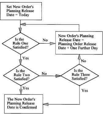
± the loading, in addition to the added ® rst operation loading of the new releasing order, should be below the pre-de® ned upper limit.Figure 1 illustrates a heuristic order release control method developed on the basis of the three loading rules. The new order’s planning release date is con® rmed only when rule 1 and either rule 2 or 3 are satis® ed. If neither one is satis® ed, the new order’s planning release date is forwarded to the next day and the logic is re-exam-ined.
The orders considered for the loading computation include the released orders and planned released orders. Loading computation for those orders whose planning order release date is today is simple: merely check the current loading status. However, loading computation for those orders that cannot be released today
(owing to the fact that none of the loading rules is satis® ed
)
will be released at a future date. Under this circumstance, what the loading status will be at that future date is unknown. Knowing the loading status at that future date requires knowledge of the released and planned release orders’ status at that future date. If the released orders at a future date have completed several operations, the loadings for those workstations having processed those completed operations should then be released as available loading at that future date. Otherwise, either partial loadings or no loading of those workcentres should be released. In this study, a heuristic algorithm, similar to the block scheduling concept (Narasimhan et al. 1995)
, is developed to accurately predict the workcentre’s loading status when an order is to be released at a future date.Step 1. Give the due-date of the order to be evaluated and determine the Quoted
Flow Time (QFT
)
. The QFT is set equal to the due date minus today. For instance, if today is day 1 and the due date of an order is on day 6, then the QFT is equal to 5 days. If it is 8 hours per day then the QFT is equal to 40 hours.Step 2. Determine the proportional operation time rate. For instance, if an order
has three operations and each operation requires processing time of 2, 3 and 5 hours respectively, the proportional operation time rate for each operation is 0.2, 0.3 and 0.5, respectively.
Step 3. Allocate the QFT to each operation on the basis of its proportional
opera-tion time rate. For instance, if the QFT is 40 hours and the proporopera-tional time rate for each operation is 0.2, 0.3 and 0.5, then the allocated QFT for each operation is 8 hours, 12 hours and 20 hours.
Figure 1. Logic of order release control.
Step 4. Determine the ending time of each operation at each workcentre. Each
operation’s ending time is the cumulative time of QFT. For instance, the ending time of operation 1 is 8 hours, ending time of operation 2 is 20 hours and ending time of operation 3 is 40 hours.
Step 5. Predict the workcentre loading at the future date. Since each operation’s
ending time at each workcentre at a future time is determined in step 4, each workcentre’s loading status for each released or planned release (future planning release is con® rmed
)
orders at any future date can be derived by checking the ending time of each operation with the future date. Three situations occur: (1)
A situation in which the ending time of the checking order’s operation is before the future date suggests that the operation was completed and its allocated loading should be deducted from the work-centre. (2)
A situation in which the starting time of the checking order’s operation is after the future date suggests that no allocated loading is deducted from the workcentre. (3)
If neither of the above two situations occurs, a linear loading deduction from the workcentre is executed. For instance, if predicting the workcentre loading after two days is desired, for the released order mentioned in the above steps, operation one’s ending time is at hour 8, it is situation one. Therefore, 2 hours of allocated loading should be deducted from the workcentre and released for other planning release orders. The operation three’s ending time is at hour 40, it is situation two; no allocated loading should be deducted from the workcentre. The operation two’s ending time is after day two, buts its starting time can be before day two, it is situation three. Moreover, a linear loading computation 3´
[
(16-
8) /12]
suggests that 2 hours of allocated loading should be deducted from the workcentre and released for other planning release orders.Step 6. Repeat steps 1 to 5 for each released and planned release orders, the
work-centre and system loading can be predicted for each order to be planned at a future date.
3. Due-date assignment rules
Three di erent due-date assignment rules (OITS, LIQ and TWK & NOP
)
are evaluated in this study. The due-date assignment procedure entails initially estimat-ing the ¯ owtime of the arrivestimat-ing order and then addestimat-ing the ¯ owtime allowance to the order’s release time (or the order’s arrival time)
.The OITS (Operation Interoperation Time Sampling
)
is modi® ed from the OFS (Operation Flowtime Sampling)
as developed by Vig and Dooley (1991)
. They con-tended that each order’s ¯ owtime is autocorrelated. The ¯ owtime length of the new completed order denoted the congestion of the system status. In this study, OITS uses the average interoperation time, total number of operations and total processing time of the three recently completed orders. The mathematical expression is as follows:Ii=K1
´
Hi+K2´
Ni+K3´
PiQ=(Q1/N1+Q2/N2+Q3/N3) /3
Hi=Q
´
NiWhere
Ii Estimated interoperation time of order i.
Ni Number of operations of order i.
Pi Total processing time of order i.
Q1
,
Q2,
Q3 Waiting time obtained from the three most recently completed orders.Ki Average waiting time of a single operation.
Hi Average waiting time of order i.
The NOP & TWK use the number of operations and total processing time of order to estimate the interoperation time. The expression equation is:
Ii= K1
´
Ni+K2´
PiThe LIQ modi® ed from the JIQ includes loading of those workcentres that the order must go through into the NOP & TWK equations. The expression equation is:
Ii= K1
´
Ni+K2´
Pi+K3´
QLiWhere QLi is the workload of the workcentres that the order goes through. In much of the previous research, the de® nition of I has been total ¯ owtime, with a variety of alternative K values studied to determine the e ect of due-date tightness. However, in this model, I is used as total interoperation time because processing time is assumed constant and becomes one of the factors in¯ uencing the interopera-tion time estimainteropera-tion. With the interoperainteropera-tion time I, the due date can then be determined by the following expression:
Fi= Pi+Ii
Di= Ri+ Fi
Where,
Fi Total ¯ owtime of order i.
Di Due-date of order i.
Ri Release date of order i.
4. Order release control adjustment
Since the interoperation time is estimated using some historical data and control parameters, some of the values will be under-estimates, which will lead to some orders being delivered late unless appropriate remedial action is taken. The simplest approach is to release those orders early. However, how do we know which order’s interoperation time is under-estimated? Since the due-date for each released order and planned releasing order in this stage is known, a backward scheduling-like checking algorithm can be applied to identify which are potential late orders.
Step 1. Give O as a set of released orders and planned releasing orders.
Step 2. Select an order Oifrom the set O which has the earliest due date. Given Oijis
a set of operations of order Oi. Assign RDi(order Oi’s planning release date
)
equal to the due date of Oi.Step 3. Schedule the last operation Oij of the order Oito its processing workcentre.
Eliminate the schedule operation from the Oij set and reset RDi as RDi minus the processing time of Oij.
Step 4. Repeat step 3 until the selected order Oihas no more operation in operation set Oij. Eliminate the selected order Oi from the order set O.
Step 5. Repeat the steps 2 to 4 until the order set O is a null set, then stop.
According to this work commitment algorithm, a schedule for the released order and the latest order release date for the releasing order can be derived. The fact that those released orders behind the schedule or those releasing orders’ planning release date lag behind the latest order release date implies that they are potential late orders. Two actions can be taken. A high priority should be given for those potential late released orders. For those potential late releasing orders, shift the release date early.
5. Scheduling rules
Three schedules are used in this study to assess the performance of integration order release control with due-date assignment rules. There are FIFS (First in ® rst service
)
, EDD (Earliest due date)
and T-SPT (Truncated shortest processing time)
. The T-SPT rule sequences jobs according to the SPT rule, except for those jobs having waited longer than a speci® ed truncation time.6. Experimental design
The experimental design consists of a three-phase investigation. First, a simula-tion model of the shop is developed and coded. Second, estimasimula-tion accuracy of the interoperation time is evaluated when the order release control is integrated with the due-date assignment rules. Finally, a factorial design is used to study whether (1
)
the proposed integration of order release control with due-date assignment rules will improve the performance of due-date assignment, and (2)
further integrating order release adjustment with order release control would increase the due-date perfor-mance. A three-factor full factorial design is used to achieve the latter task. The design includes three due-date assignment rules (NOP & TWK, LIQ and OITS)
, three scheduling rules (FIFS, EDD and T-SPT)
and three order release models. The three order release models are: (1)
Basic model, in which three due-date assignment rules consider the order arrival time as the order release time; (2)
Control model, in which three due-date assignment rules integrate with the order release control method developed in§2. This implies that the order release time is either equal to or greater than, the order arrival time. Orders are released to the shop ¯ oor based on the order release control method; and (3)
Adjustment model, in which the control model integrates with the order release control adjustment developed in§4. 6.1. Shop modelThe shop model developed by Vig and Dooley (1991
)
is adopted here. The shop has ® ve unique workcentres. Each workcentre contains one machine. The arrival of orders to the shop is random with interarrival times that are exponentially distrib-uted with a mean of 1.2 hours. Arriving orders are assigned from one to ten opera-tions with uniform distribution. No successive operaopera-tions performed at the same workcentre are permitted. The operation time is also random variables from a 2-Erlang distribution with a mean of 1.0 hour. Further assumptions regarding the shop model are described below:(1
)
A speci® c work centre has constant availability over time. For simplicity in modelling machine breakdowns and maintenance are not considered.(2
)
The model does not include assembly operations. All orders consist of sequential operations which are independent of other orders.(3
)
Each work centre is unique in the job shop.(4
)
Each operation must be performed at the designated work centre. Alternative routeings are not considered.(5
)
Preemption of an operation is not allowed. An order cannot be removed from a queue until the current operation at the work centre is completed. (6)
Only a single operation can be processed at a time for a particular order. (7)
Work centres can process only one operation at a time.The computer simulation model was programmed in SLAMSYSTEM (Pritsker 1991
)
, a simulation analysis language for modelling general systems.6.2. Estimation accuracy of interoperation time
Steady-state simulation runs of 120 000 hours (i.e. 100 000 jobs completed
)
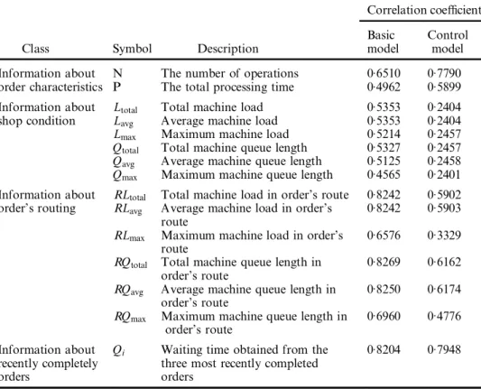
are generated. Of the completed orders, 5% are randomly selected as samples to ensure that the observations are approximately independent. With correlation analysis, those relative variables (shop ¯ oor and order information)
that a ect the quality of interoperation time estimation for basic model and control model can be found. Table 1 summarizes the analysis results. Based on those results, we can conclude the following:Correlation coe cient Class Symbol Description Basicmodel Controlmodel Information about
order characteristics NP The number of operationsThe total processing time 0 .6510 0.4962 0
.7790 0.5899 Information about Ltotal Total machine load 0.5353 0.2404
shop condition Lavg Average machine load 0.5353 0.2404
Lmax Maximum machine load 0.5214 0.2457
Qtotal Total machine queue length 0.5327 0.2457
Qavg Average machine queue length 0.5125 0.2458
Qmax Maximum machine queue length 0.4565 0.2401
Information about RLtotal Total machine load in order’s route 0.8242 0.5902
order’s routing RLavg Average machine load in order’s
route 0
.8242 0.5903 RLmax Maximum machine load in order’s
route 0
.6576 0.3329
RQtotal Total machine queue length in
order’s route 0
.8269 0.6162 RQavg Average machine queue length in
order’s route 0
.8250 0.6174 RQmax Maximum machine queue length in 0.6960 0.4776
order’s route Information about
recently completely orders
Qi Waiting time obtained from the
three most recently completed orders
0.8204 0.7948
Table 1. Correlation coe cients of information items and interoperation time.
(1
)
The number of information items that are signi® cant to the interoperation time estimation for the control model are less than for the basic model. Therefore, fewer information items are required in estimating the interopera-tion time in a control model.(2
)
Information about shop’s condition is less signi® cant in estimating the inter-operation time for the control model. This ® nding veri® es that order release control is critical in stabilizing the shop ¯ oor.(3
)
Information regarding the order characteristics is critical in interoperation time for both models, particularly the number of operations.(4
)
Regardless of the model, information regarding the order’s route is more useful than the other information items when estimating interoperation time.6.3. Due-date assignment rules’ parameters estimation
Since three di erent scheduling rules and di erent order sequences will be generated, the parameter values for each interoperation time estimation equation should be estimated individually. In this paper, a regression model is used to derive the parameters’ value for each interoperation time estimation equation with the input of the simulation results from the initial simulation run described in §6.2. Tables 2 and 3 summarize the regression analysis results.
Scheduling rule Due-date rules Parameter value
FIFS NOP & TWK Ii= 0.172+ 9.543Ni
-
0.160PiLIQ Ii=
-
17.446+4.742Ni-
0.195Pi+0.324RLi,totalOITS Ii= 0.212+ 0.730Hi+2.817Ni
-
0.197PiEDD NOP & TWK Ii=
-
7.450+1.840Ni+8.505PiLIQ Ii=
-
25.344-
2.508Ni+ 8.433Pi+0.202RLi,totalOITS Ii=
-
8.126+0.548Hi-
2.614Ni+ 8.576PiT-SPT NOP & TWK Ii= 0.595+ 1.726Ni+ 5.018Pi
LIQ Ii=
-
13.588-
2.050Ni+ 4.686Pi+0.389RLi,totalOITS Ii= 1.411+ 0.636Hi
-
2.590Ni+4.916PiTable 2. Parameters estimation for basic model.
Scheduling rule Due-date rules Parameter value FIFS NOP & TWK Ii= 0.493+ 8.269Ni
-
0.322PiLIQ Ii=
-
4.795+6.886Ni-
0.289Pi+0.056RLi,totalOITS Ii= 0.307+ 0.503Hi+4.284Ni
-
0.314PiEDD NOP & TWK Ii=
-
14.424+1.351Ni+7.572PiLIQ Ii=
-
16.185+0.848Ni+7.600Pi+0.009RLi,totalOITS Ii=
-
14.432+0.068Hi+ 1.003Ni+7.566PiT-SPT NOP & TWK Ii= 0.753+ 0.693Ni+ 4.546Pi
LIQ Ii=
-
3.442-
0.474Ni+4.536Pi+0.070RLi,totalOITS Ii= 0.828+ 0.287Hi
-
0.900Ni+4.589PiTable 3. Parameters estimation for control model.
6.4. Experimental procedure
Two three-factor full factorial experimental designs are used to evaluate whether the control model and adjustment model will enhance the performance of the due-date assignment rule. Experiment One compares the control model with the basic model. Experiment Two compares the control model with the adjustment model. Both designs require eighteen experiments to investigate all factor level combina-tions.
6.4.1. Experiment One
The simulation was run 150 000 hours with a warm-up period of 3000 hours to reach steady-state conditions. The data was then collected to evaluate the perfor-mance of the three due-date assignment rules. The perforperfor-mance measures are aver-age ¯ owtime, averaver-age lateness, standard deviation of lateness, averaver-age tardiness and % of tardy jobs.
The experiments were performed using 30 replications of each treatment. Tables 4 and 5 summarize the results of the eighteen experiments. The analysis of variance (ANOVA
)
(Tables 6 and 7)
indicates that at a 0.05 signi® cance level, all three sources of variation (release, scheduling rule and due-date assignment)
and all two wayScheduling
rule Due-date rules ¯ ow timeAverage Averagelateness Std. dev.lateness tardinessAverage % tardyjobs FIFS NOP & TWK 64.40 7.29 35.81 32.56 49.73
LIQ 61.95 2.33 22.16 17.26 50.79 OITS 64.41 2.36 26.34 21.88 47.66 EDD NOP & TWK 55.84 0.90 24.70 21.03 45.61 LIQ 55.15 0.38 13.89 10.83 50.70 OITS 50.93
-
0.48 16.07 12.24 46.96 T-SPT NOP & TWK 43.71 0.42 33.76 30.53 38.27 LIQ 43.61-
0.12 25.13 17.39 46.45 OITS 43.61 0.23 28.26 22.61 40.59Table 4. Experimental results of basic model.
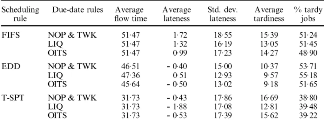
Scheduling
rule Due-date rules ¯ ow timeAverage Averagelateness Std. dev.lateness tardinessAverage % tardyjobs FIFS NOP & TWK 51.47 1.72 18.55 15.39 51.24
LIQ 51.47 1.32 16.19 13.05 51.45 OITS 51.47 0.99 17.23 14.27 48.90 EDD NOP & TWK 46.51
-
0.40 15.00 10.37 53.71 LIQ 47.36 0.51 12.93 9.57 55.18 OITS 45.64-
0.50 13.02 9.18 51.65 T-SPT NOP & TWK 31.73-
0.43 17.86 16.69 38.80 LIQ 31.73-
1.88 17.08 12.81 39.48 OITS 31.73-
0.53 17.39 15.62 39.22Table 5. Experimental results of control model.
interactions (except A
´
C)
are signi® cant. This concludes that the performance of due-date assignment can be improved in a stable system which can be achieved by an appropriate order releasing method. Although A´
C is not signi® cant at a 0.05 signi® cance level, its standard deviation of lateness is still quite signi® cant.The performance comparison for basic and control model was analysed by paired
t tests, with those results listed in Table 8. This table reveals that for the standard
deviation of lateness, the control model is markedly better than the basic model. This ® nding suggests that the control model increases the accuracy of the due-date assign-ment (or ¯ owtime estimation
)
. However, for the average lateness, except for the combination of T-SPT and LIQ, the control model is either better than the basic model or both are not signi® cantly di erent. In contrast, for the % of tardy orders, except the combination of T-SPT and LIQ, the basic model is either better than the control model or both are not signi® cantly di erent. However, if the control model uses the basic model’s due-date rules’ parameter value to estimate the interoperation time, the percentage of tardy orders will then be reduced signi® cantly. This is because the interoperation time of the basic model is greater than that of the control model. For average tardiness and average ¯ owtime, the control model is signi® cantly better than the basic model.Source of variation Degrees offreedom squaresSum of squareMean F Pr>F Release model (A) 1 260.31 260.31 15.30 0.0001 Scheduling rules (B) 2 978.92 489.46 28.77 0.0001 Due-date assignment 2 173.28 86.64 5.09 0.0064 rules (C) A´ B 2 118.83 59.42 3.49 0.0311 A´ C 2 94.87 47.44 2.79 0.0624 B´ C 4 195.60 48.90 2.87 0.0225 A´ B´ C 4 125.49 31.37 1.84 0.1190 Error 522 8879.28 17.01
Table 6. ANOVA for average lateness.
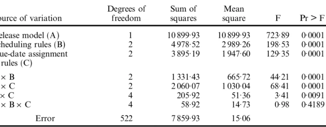
Source of variation Degrees offreedom squaresSum of squareMean F Pr>F Release model (A) 1 10 899.93 10 899.93 723.89 0.0001 Scheduling rules (B) 2 4 978.52 2 989.26 198.53 0.0001 Due-date assignment 2 3 895.19 1 947.60 129.35 0.0001 rules (C) A´ B 2 1 331.43 665.72 44.21 0.0001 A´ C 2 2 060.07 1 030.04 68.41 0.0001 B´ C 4 205.92 51.36 3.41 0.0091 A´ B´ C 4 58.92 14.73 0.98 0.4189 Error 522 7 859.93 15.06
Table 7. ANOVA for standard deviation of lateness.
6.4.2. Experiment Two
Experiment Two is the same as experiment one except that the basic model changes to the adjustment model in which the order release date is adjustable. Table 9 summarizes the results. Since the adjustment model only addresses the average tardiness and % of tardy orders, Table 10 provides only the performance comparison results for the control model and the adjustment model. Table 10 indi-cates that except for the combination of EDD and OITS, with respect to the per-formance of the average tardiness, the control model is signi® cantly better than the adjustment model or both are not signi® cantly di erent. However, for the percentage of tardy orders, the performance depends on scheduling rules. For FIFS and EDD, the adjustment model is better than the control model, since the adjustment model concentrates on due-date performance. However, combining with the T-SPT, the adjustment policy is disrupted, thereby making the control model better than the adjustment model.
Scheduling
rule Due-daterules ¯ ow timeAverage Averagelateness Std. dev.lateness tardinessAverage % tardyjobs FIFS NOP & TWK*(CONTROL) *(CONT ROL) *(CONTROL) *(CONTROL) /
LIQ *(CONTROL) **(CONTROL)*(CONTROL) *(CONTROL) / OITS *(CONTROL) *(CONT ROL) *(CONTROL) *(CONTROL) / EDD NOP & TWK*(CONTROL) / *(CONTROL) *(CONTROL) **(BASIC)
LIQ *(CONTROL) / *(CONTROL) *(CONTROL) *(BASIC)
OITS *(CONTROL) / *(CONTROL) *(CONTROL) **(BASIC)
T-SPT NOP & TWK*(CONTROL) / *(CONTROL) *(CONTROL) /
LIQ *(CONTROL) **(BASIC) *(CONTROL) *(CONTROL) *(CONTROL)
OITS *(CONTROL) / *(CONTROL) *(CONTROL) / / Not statistically di erent.
* Statistically di erent at signi® cance level of 0.01 ** Statistically di erent at signi® cance level of 0.1. ()Model in parentheses is a better model.
Table 8. Performance comparisons for basic and control models.
Scheduling
rule Due-daterules ¯ ow timeAverage Averagelateness Std. dev.lateness tardinessAverage % tardyjobs FIFS NOP & TWK 58.22 0.43 25.43 21.12 44.63
LIQ 54.09 1.87 20.89 17.42 50.30 OITS 60.62
-
3.63 24.28 17.81 40.38 EDD NOP & TWK 49.48-
3.36 15.50 9.72 44.50 LIQ 51.04 0.10 13.98 9.58 52.97 OITS 50.72-
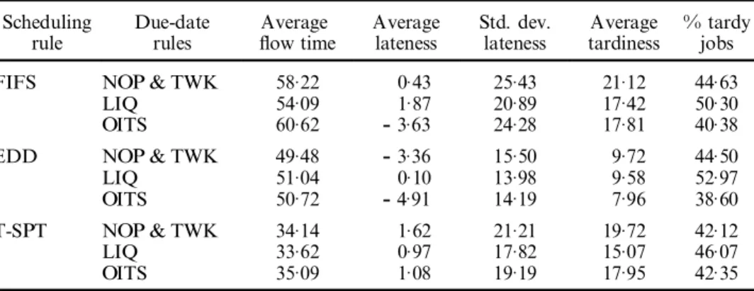
4.91 14.19 7.96 38.60 T-SPT NOP & TWK 34.14 1.62 21.21 19.72 42.12 LIQ 33.62 0.97 17.82 15.07 46.07 OITS 35.09 1.08 19.19 17.95 42.35Table 9. Experimental results of adjustment models.
7. Conclusions
This study integrates the order releasing control method with due-date assign-ment rules. An order release control mechanism has been presented which aims to control manufacturing lead times. Several experimental designs are also performed to evaluate the e ectiveness of integrating the due-date assignment. Based on the results in this study, we can conclude the following:
(1
)
Integrating of order release control with duedate assignment rules signi® -cantly improve the average ¯ owtime estimation, due-date performance in average lateness and standard deviation of lateness.(2
)
The integrated due-date assignment model, combined with the order release adjustment method, decreases the percentage of tardy orders when FIFS and EDD scheduling rules are used.(3
)
Integrating order release control with due-date assignment rules reduces the number of shop ¯ oor information items in estimating the interoperation time. This subsequently increases the estimation accuracy of the interopera-tion time. However, the estimainteropera-tion accuracy of the interoperainteropera-tion time will increase the accuracy of the due-date assignment model.Results in this study con® rm the notion that integrating the order release control method with due-date assignment rules will signi® cantly enhance the estimation accuracy of interoperation time and due-date performance of due-date assignment rules.
References
Bobrow ski, P. M., 1989, Implementing a loading heuristic in a discrete release job shop. International Journal of Production Research,27, 1935± 1948.
Conw ay, R. W., Ma xw ell, W. L., and Miller, L. W., 1967, Theory of Scheduling ( Reading, MA: Addison-Wesley).
Eilon, S., and Chow dhury, I. G., 1976, Due dates in job shop scheduling. International Journal of Production Research,14, 223± 237.
Hendry, L. C., and Wong, S. K., 1994, Alternative order release mechanisms: a comparison by simulation. International Journal of Production Research,32, 2827± 2842.
Scheduling rule Due-date rules Average tardiness Percent tardy jobs FIFS NOP & TWK *(CONTROL) *(ADJUST)
LIQ *(CONTROL) /
OITS *(CONTROL) *(ADJUST)
EDD NOP & TWK / *(ADJUST)
LIQ / /
OITS *(ADJUST) *(ADJUST)
T-SPT NOP & TWK *(CONTROL) **(CONTROL)
LIQ *(CONTROL) *(CONT ROL)
OITS *(CONTROL) *(CONT ROL)
/ Not statistically di erent.
* Statistically di erent at signi® cance level of 0.01. ** Statistically di erent at signi® cance level of 0.1 ()Model in parentheses is a better model.
Table 10. Performance comparisons for control and adjustment models.
Irastorz a, J. C., and Dea ne, R. H., 1974, A loading and balancing methodology for job shop control. AIIE Transactions,6, 302± 307.
Ling aya t, S., Mittenthal, J., and O’Keefe, R. M., 1995, An order release mechanism for a ¯ exible ¯ ow system. International Journal of Production Research,33, 1241± 1256.
Loc kett, A. G., and Muhlemann, A. P., 1978, A problem of aggregate scheduling: an application for goal programming. International Journal of Production Research, 16, 127± 135.
Melnyk, S. A., and Ra gatz, G. L., 1989, Order review/release: research issues and perspec-tives. International Journal of Production Research,27, 1081± 1096.
Narasimhan, S. L., Mclea vey, D. W., and Billing ton, P. J., 1995, Production Planning and Inventory Control (Englewood Cli s, NJ: Prentice Hall).
Onu r, L., and Fa bryc ky, W. J., 1987, An input/output control system for the dynamic job shop. IIE Transactions, 19, 88± 97.
Philipoom, P.R., and Fry, T. D., 1992, Capacity-based order review/release strategies to improve manufacturing performance. International Journal of Production Research,
30, 2559± 2572.
Pritsker, A. B., 1991, Introduction to Simulation and S L AM II, 3rd edn (W. Lafayette, IN: Systems Publishing).
Rag atz, G. L., and Mabert, V. A., 1988, An evaluation of order release mechanisms in a job-shop environment. Decision Sciences,19, 167± 189.
Rag atz, G. L., 1989, A note of workload-dependent due date assignment rules. Journal of Operations Management,8, 377± 384.
Rod erick, L. M., Phillips, D. T., and Hog g, G. L., 1992, A comparison of order release strategies in production control systems. International Journal of Production Research,
30, 611± 626.
Vig, M. M., and Dooley, K. J., 1991, Dynamic rules for due-date assignment. International Journal of Production Research,29, 1361± 1377.
Vig, M. M., and Dooley, K. J., 1993, Mixed static and dynamic ¯ owtime estimates for due-date assignment. Journal of Operations Management,2, 67± 79.
Zapfel, G., and Missbau er, H., 1993, New concepts for production planning and control. European Journal of Operational Research,67, 297± 320.