具自動建構特性之模糊與類神經網路控制架構於非線性動態系統之應用

國

立

交

通

大

學

電機與控制工程系

博 士 論 文

具自動建構特性之模糊與類神經網路控制架構於

非線性動態系統之應用

Fuzzy and Neural Network Control Schemes with

Automatic Structuring Process for Nonlinear Dynamic

Systems

研 究 生：陳品程

指導教授：李祖添 教授

王啟旭 教授

具自動建構特性之模糊與類神經網路控制架構於非線性動態

系統之應用

Fuzzy and Neural Network Control Schemes with Automatic

Structuring Process for Nonlinear Dynamic Systems

研 究 生：陳品程 Student : Pin-Cheng Chen

指導教授：李祖添 Advisor(s) : Tsu-Tian Lee

王啟旭

Chi-Hsu Wang

國 立 交 通 大 學

電機與控制工程系

博 士 論 文

A Dissertation

Submitted to Department of Electrical and Control Engineering College of Electrical Engineering

National Chiao Tung University in partial Fulfillment of the Requirements

for the Degree of Doctor of Philosophy

in

Electrical and Control Engineering

October 2008

Hsinchu, Taiwan, Republic of China

具自動建構特性之模糊與類神經網路控制架構於非

線性動態系統之應用

研究生：陳品程

指導教授：李祖添 博士

王啟旭 博士

國立交通大學電機與控制工程系博士班

摘

要

為解決非線性系統控制問題，本論文發展兩個嶄新的控制架構。首先針

對非仿射的非線性動態系統，提出具自我建構特性的強健適應性模糊控制

架構。此架構中的控制器包含一個自我建構的模糊控制器和一個強建控制

器。自我建構的模糊控制器用來近似未知的系統非線性，並可以自動刪除

及產生模糊規則以建立簡潔的模糊規則庫;強健控制器用來達成 L

2

追蹤表

現，並抑制誤差至要求的範圍以使系統穩定。我們舉出四個例子顯示此控

制架構不但能有良好的控制表現，也可大量減少運算量。其次針對仿射的

非線性動態系統，提出使用以霍普菲爾為基礎的動態類神經網路的直接適

應性控制架構。在此架構中，以霍普菲爾為基礎的動態類神經網路用來近

似一個理想控制器；監督控制器則用來抑制近似誤差和外界干擾的影響。

藉由 Lypunov 方法可堆導出適應法則，用以調整網路的權重值使得系統穩

定。經由適當地選取參數，可將追蹤物差抑制到要求的範圍內。經由模擬

證實了此架構的可行性及良好效果。僅含一個神經元的以霍普菲爾為基礎

的動態類神經網路使得此架構易於以硬體實現，另外，我們亦探討由無自

我回授神經元建構而成的以霍普菲爾為基礎的動態類神經網路。經比較發

現，採用具有自我回授神經元的以霍普菲爾為基礎的動態類神經網路之控

制架構，其控制表現較佳。值得注意的是，本論文中所提出的自我建構模

糊系統和固定架構的以霍普菲爾為基礎的動態類神經網路皆不需要專家的

知識或是試誤過程來決定其架構，因此解決了模糊系統和類神經網路的架

構問題。

Fuzzy and Neural Network Control Schemes with Automatic

Structuring Process for Nonlinear Dynamic Systems

Student：Pin-Cheng Chen

Advisor(s): Dr. Tsu-Tian Lee

Dr. Chi-Hsu Wang

Department of Electrical and Control Engineering

National Chiao Tung University

ABSTRACT

In this dissertation, two novel control schemes are proposed to solve the control problems of nonlinear systems. The first is a robust adaptive self-structuring fuzzy control (RASFC) scheme for nonaffine nonlinear systems, and the second is a direct adaptive control scheme using Hopfield-based dynamic neural network (DACHDNN) for affine nonlinear systems. The RASFC scheme is composed of a robust adaptive controller and a self-structuring fuzzy controller. The design of the self-structuring fuzzy controller design utilizes a novel self-structuring fuzzy system (SFS) to approximate the unknown plant nonlinearity, and the SFS can automatically grow and prune fuzzy rules to realize a compact fuzzy rule base. The robust adaptive controller is designed to achieve a L2 tracking performance with a desired attenuation level to stabilize the closed-loop system. Four examples are presented to show that the proposed RASFC scheme can achieve favorable tracking performance and relieve heavy computational burden. In the DACHDNN, a Hopfield-based dynamic neural network is used to approximate the ideal controller, and a compensation controller is used to suppress the effect of approximation error and disturbance. The weightings of the Hopfield-based dynamic neural network are on-line tuned by the adaptive laws derived in the Lyapunov sense, so that the stability of the closed-loop system can be guaranteed. The tracking error can be attenuated to a desired level by adequately selecting some parameters. The case of Hopfield-based neural network without the self-feedback loop is also studied and shown to have inferior results than those of Hopfield neural network with the self-feedback loop. Simulation results illustrate the applicability of the proposed control scheme. The Hopfield-based dynamic neural network with a parsimonious structure has the best potential be realized in hardware. It should be emphasized

that the self-structuring property of the SFS and the fixed parsimonious structure of the DACHDNN eliminate the need for expert’s knowledge or error-trial process and thus provide perfect solutions to the structuring problems of fuzzy systems and neural networks, respectively.

Acknowledgement

經過了五年多的日子，終於能順利取得博士學位，心中百感交集，除了喜悅之外， 更充滿了感謝。謝謝我的指導教授李祖添老師。除了在研究上的指導，老師自律嚴謹的 為人處世、治學態度是我最好的典範。幾次在老師所承辦的大型國際學術會議中參與準 備工作，讓我學習到做事的方法以及開闊的國際視野。雖然老師非常繁忙，對於我們的 生活、畢業、未來出路方面，老師仍然相當關心並盡力給予我們幫助。謝謝我的另外一 位指導教授王啟旭老師。王啟旭老師深具創意的思考為我的研究提供了莫大的啟發，與 學生相處時親切爽朗的態度令人如沐春風，對於我的生活及身體健康的關懷，更使人備 感溫暖。對於兩位老師的栽培之恩，我永生難忘。 感謝我的口試委員：徐保羅教授、蘇順豐教授、王偉彥教授、以及呂藝光教授，對 於我的畢業論文提供了許多寶貴的意見及不同的思考方向，使得論文內容能更加完整與 正確。其中尤其要感謝王偉彥老師，自從我從輔大碩士班畢業以後，您仍然不吝給予我 許多指導及幫助，身為您的學生我深感幸運。 此外，還要感謝許駿飛學長，在您的指導下經過長時間的相互討論與分享，才能慢 慢建立起我的研究理論基礎，沒有您的熱忱幫助，我不會這麼順利地取得博士學位。謝 謝炳榮，七年來無論在研究或生活上，都合作無間，互相幫忙、彼此關懷；謝謝偉竹， 總計八年的室友，後四年有炳榮的加入，三個人一起瘋癲笑鬧、一起快樂傷心過的青春， 永難忘懷。謝謝我所深愛過的，那些快樂和悲傷都是我珍貴的寶物。謝謝彭昭暐學長、 溫裕弘學長、保村學長、李宜勳學長、欣翰、文真、雅齡、逸幗、詠健、東璋、得裕、 堃能、其他的學弟妹們，有你們在，研究生活更充實愉快。謝謝助理天鳳、鳳儀、佳明， 謝謝在這段期間所有關心我的朋友和直接或間接給予我幫助的人們。 最後要謝謝我最愛的父母與家人，你們給予我無條件的愛，永遠支持我、給予我鼓 勵，是我最安全的避風港。我願能以同樣深切的愛回報你們，並與你們分享今日我小小 的成就。

Table of Contents

Abstract in Chinese i

Abstract in English iii Acknowledgement v Table of Content ………. vi

List of Figures ………. viii

List of Tables ………. x

1. Introduction 1.1 Background and Motivation……….. 1

1.2 Major Works……….. 4

1.3 Dissertation Overview……… 6

2. Robust Adaptive Self-structuring Fuzzy Control Design for Nonaffine Nonlinear Systems……… 7

2.1 Problem Formulation………. 7

2.2 Self-structuring Fuzzy System………... 9

2.2.1 Description of Fuzzy System………. 9

2.2.2 Structure Learning Algorithm……… 10

2.3 Design of RASFC……….. 16

2.3.1 Fuzzy Approximation………. 16

2.3.2 Parameter Learning Algorithm………... 20

2.4 Simulation Results……….. 25

3. Direct Adaptive Control Design Using Hopfield-Based Dynamic Neural Network for Affine Nonlinear Systems……….. 40 3.1 Hopfield-Dynamic Neural Network………... 40

3.1.1 Description of DNN Model……… 40

3.1.2 Hopfield-based DNN Approximator……….. 42

References 62

Vita 67

Publication List 68

3.3 Design of DACHDNN………... 44

3.4 Simulation Results………. 50

3.5 Performance analysis of Hopfield-based DNNs with and without the

self-feedback loop……….. 55

List of Figures

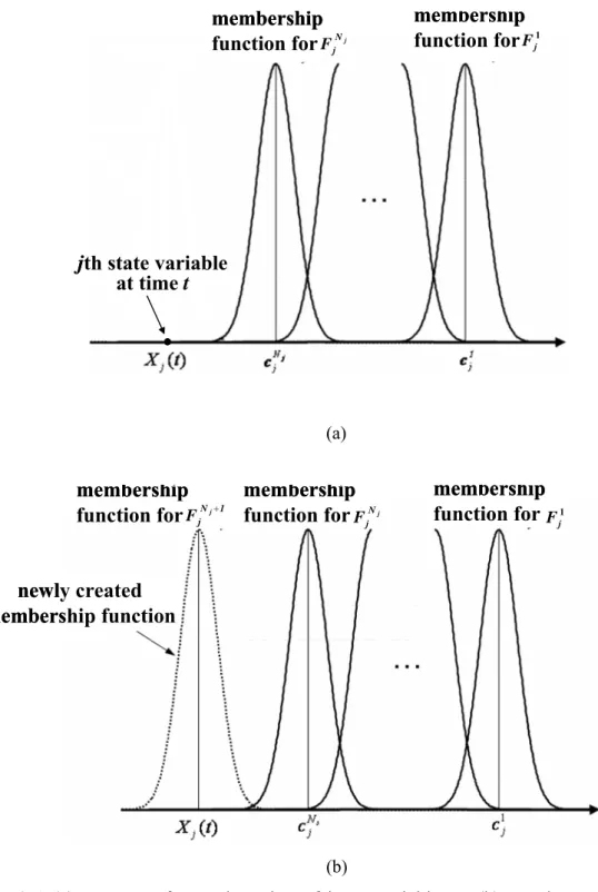
Fig. 2-1(a) Improper fuzzy clustering of input variable Xj………... 11

Fig. 2-1(b) Newly created membership function………..………. 11

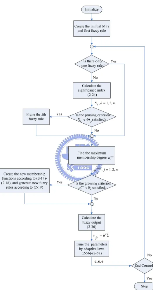
Fig. 2-2 The flowchart of the self-structuring algorithm for the SFS…………... 15

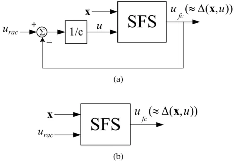
Fig. 2-3(a) The recurrent fuzzy system………. 17

Fig. 2-3(b) The static fuzzy system………... 17

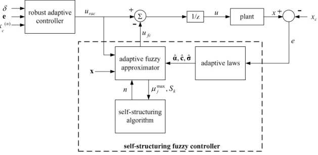
Fig. 2-4 The block diagram of RASFC for nonaffine nonlinear systems……… 24

Fig. 2-5 Approximation results in Example 2-1. (a) is approximation results of Condition 1a; (b) is approximation results of Condition 1b; (c) is approximation results of Condition 1c; (d) is the approximation error;

(e) is the number of fuzzy rules……….. 26-27

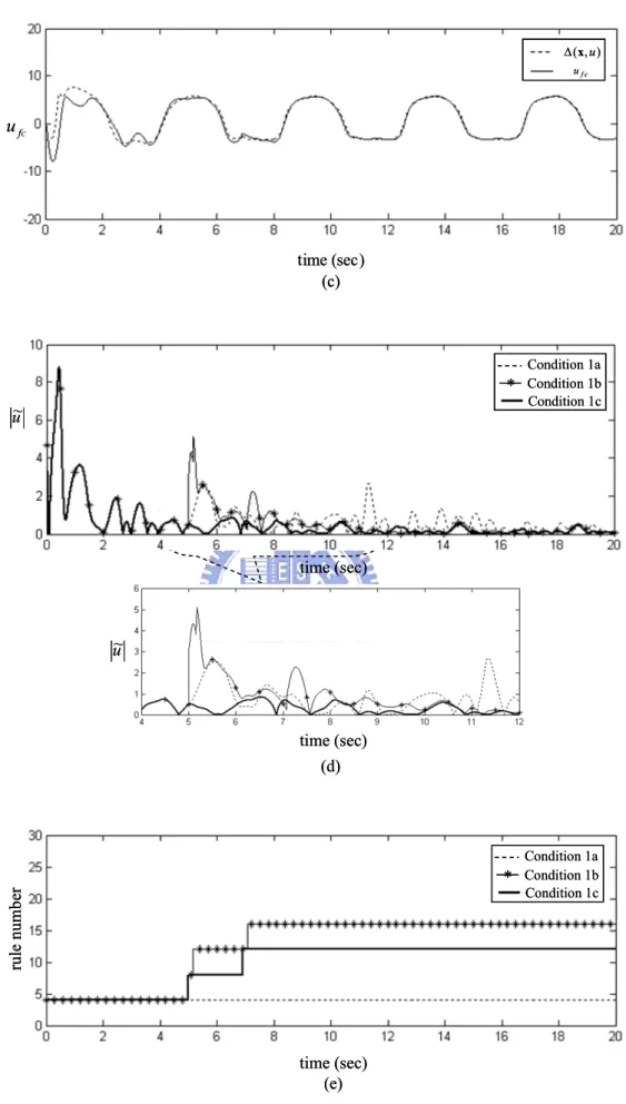
Fig. 2-6 Approximation results in Example 2-2. (a) is approximation results of Condition 1a; (b) is approximation results of Condition 1b (c) is the approximation error; (d) is the number of fuzzy rules; (e) is the contribution and significance index of a certain rule……….. 29-31 Fig. 2-7 Simulation results of Case 3a in Example 2-3. (a) is the response of

state x1; (b) is the response of state x2; (c) is the control input; (d) is the

number of fuzzy rules……….. 32-33

Fig. 2-8 Simulation results of Case 3b in Example 2-4. (a) is the response of state x1; (b) is the response of state x2; (c) is the control input; (d) is the

number of fuzzy rules……….. 33-34

Fig. 2-9 Simulation results of Case 4a in Example 2-4. (a) is the response of state x1; (b) is the response of state x2; (c) is the control input; (d) is the

number of fuzzy rules……….. 36-37

Fig. 2-10 Simulation results of Case 4b in Example 2-4. (a) is the response of state x1; (b) is the response of state x2; (c) is the control input; (d) is the

number of fuzzy rules…………...………... 37-38

Fig. 3-1 The structure of the dynamic neural network………. 41

Fig. 3-2 The Block diagram of the DACHDNN……… 45

Fig. 3-3 The Electric circuit of Hopfield-based DNN containing only a single

Fig. 3-4 The Phase plane of uncontrolled chaotic system……… 51 Fig. 3-5 Simulation results of Example 3-1. (a) is the response of state x1; (b) is

the response of state x2; (c) is the control input; (d) show the trained

w e i g h t i n g s … … … . . . 52-53 Fig. 3-6 Simulation results of Example 3-2. (a) is the response of state x1; (b) is

the response of state x2; (c) is the response of state x3; (d) is the control

input; (e) show the trained weightings………... 54-55

Fig. 3-7 Simulation results of Example 3-1 using Hopfield-based DNN without the feedback loop. (a) is the response of state x1; (b) is the response of

state x2; (c) is the norm of tracking error……….. 57

Fig. 3-8 Simulation results of Example 3-3 using Hopfield-based DNN without feedback. (a) is the response of state x1; (b) is the response of state x2;

List of Tables

Table 2-1. Three conditions in Example 2-1……….... 25

Table 2-2 Two conditions in Example 2-2………... 28

Table 2-3 Comparison between two cases in Example 2-3………. 31

Chapter 1

Introduction

1.1 Background and Motivation

Recently, control system design for nonlinear systems has attracted a lot of research interests. Many remarkable results have been obtained, including feedback linearization [1], adaptive backstepping design [2], fuzzy logic control [3], neural network control [4], and fuzzy-neural control [5]. In general, nonlinear systems can be classified into two categories, affine nonlinear systems, i.e., systems characterized by inputs appearing linearly in the system state equation, and nonaffine nonlinear systems, where the control input appears in a nonlinear fashion [6]. Many systems encountered in engineering, by nature or by design, are affine systems, such as inverted pendulum systems [3], mass-spring-damper system [7-8], chua’s circuit [9-10], straight-arm robot [11], DC-to-DC converter [12], etc. On the other hand, nonaffine systems are quite common in the real world, such as Van de Pol oscillator [13-15], magnetic servo levitation systems [16], aircraft flight control systems [17], biochemical process [18], etc.

Fuzzy system (FS) which adopts human experience and human decision-making behavior has been widely recognized as a powerful tool in industrial control, commercial prediction, image processing applications, etc. [19-21]. To build a FS, there are two different phases to be carried out. The first is the structuring phase, which is used to construct the structure of FS, and the second is the parameter phase, which is used to determine the parameters of FS. Constructing the structure of FS is mainly to determine the optimal partition of fuzzy sets and the minimum number of fuzzy rules to achieve favorable performance. The adjustments of the parameters involve the tuning of the consequences of the fuzzy rules, the centers, widths, slopes of membership functions, etc. Traditionally, these two phases are performed by human experts or experienced operators. However, consulting experts may be difficult and expert knowledge is either unavailable or not helpful enough to achieve favorable performance. Having achieved many practical successes, fuzzy control (FC) using FS has still not been viewed as rigorous because it lacks a systematic design procedure to determine proper membership functions with fuzzy rules, and the way to guarantee the

global stability. Adaptive fuzzy control (AFC) has been extensively studied to tackle this problem [21-26]. Adaptive fuzzy system can approximate the unknown system dynamics or ideal controller through learning in the Lyapunov sense, and thus the global stability can be guaranteed.

Although the control performances in [21-26] are acceptable, the structures of the FSs need to be predefined by a time-consuming trial-and-error process. Generally speaking, a more favorable performance requires more fuzzy rules, but this may lead to heavy computational burden. On the contrary, a FS with small fuzzy rule base may result in a poor approximation.

To solve the problem of structure determination, many researchers have focused their efforts on the self-structuring fuzzy system (SFS) and obtained some valuable results [27-31]. In [27], the structure learning phase aims at minimizing the number of rules generated and the number of fuzzy sets in the universe of discourse. A structure learning algorithm is proposed based on fuzzy similarity measure, and fuzzy rules can be created from the training data. In [28], the structure identification is accomplished automatically based only on Q-learning, which is the most important category of reinforcement learning algorithm. The basic fuzzy rules are used as starting points to reduce the number of iterations used to find an optimal fuzzy controller. In [29], the firing strength of a rule is used as the degree measure to judge whether or not to simultaneously generate a new membership function for every input variable (or equivalently, to generate a new rule.) Then, if the newly generated membership of the first input variable fails to pass the similarity checking, all new membership functions are abandoned. In [30], parameter and structure learning are performed sequentially for the proposed fuzzy neural network. That is, the fuzzy neural network is initially constructed to contain all possible fuzzy rules, and then the parameter training is performed. After the parameter training is completed, a pruning process is performed to delete redundant rules and thus leads to a concise fuzzy rule base. Note that the initially constructed rule base contains incompatible rules, i.e., the rules with the same antecedent but different consequents. The rule pruning strategy is that if the centroid of a set of incompatible rules is in the support of a consequent (an output fuzzy set), the corresponding fuzzy rule is remained and all other incompatible rules are pruned. In [31], the authors modified the fuzzy neural network proposed in [30] and proposed rule pruning scheme that always produces a rule set without incompatible rules.

However, although some achievements have been made in these works, there are still some problems need to be solved. In [27], the performance of the proposed neural fuzzy

system is acceptable, but the back propagation learning algorithm cannot guarantee the global stability. In [28], during the training process, prior knowledge of fuzzy rules is needed to keep safe operation of the controlled system with fast convergence speed of parameters. In [29], the simplified similarity checking to reduce the complexity of the algorithm may weaken the power of the checking itself. In [30], because the connection weights of the network are unrestricted in sign, incompatible rules may be retained even rule pruning process is performed. This is contradictory to the basic design philosophy of fuzzy systems. Besides, the proposed sequential learning scheme is suitable for offline instead of online operation. In [31], although the fuzzy neural network in [30] is modified to guarantee a compatible rule base, the searching space for the connection weights is restricted to R+. This may harm the capability of the proposed network to lower the value of residual square error. The common drawback in [27-31] is that the structuring learning phase conducts either rule generation or rule reduction, instead of both.

Recently, research interest has been increasing towards the usage of neural network (NN) for controlling a wide class of complex nonlinear systems under the restriction that complete model information is not available [32-36]. Due to their massive parallelism, fast adaptability, and inherent approximation capabilities, NN seems to be a feasible solution to the control problem of nonlinear systems.However, the structuring problem of NNs, which mainly refers to determining the number of the neurons, is an annoying problem. This choice faces a similar dilemma as the choice of fuzzy rule number in the FS design. Generally speaking, more favorable performance requires more neurons, but this may lead to a complicated network structure and heavy computational burden. On the contrary, an NN with too few neurons in the hidden layer(s) will make it hard for the network to recognize the relationships between the output and input parameters, and thus result in a poor approximation. In general, the number of neurons is chosen empirically and apparently not optimized.

Two major classes of NNs, static and dynamic NNs, have become enormously important in recent years. In static NNs, which are also called feedforward NNs, signals flows from the input units to the output units in a forward direction. In dynamic NNs, dynamic elements are involved in the structure of the NN, for example, in the form of feedback connections. Some static neural networks (SNNs), such as feedforward fuzzy neural network (FNN) or feedforward radius basis function networks (RBFN), are frequently used as powerful tools for modeling the ideal control input or nonlinear functions of systems. Some results are shown in [39-42]. Although feedforward FNNs and RBFNs have achieved much theoretical success, they leave some space for improvement. The complex structures of feedforward FNNs and

RBFNs make the practical implementation of the control schemes infeasible, and usually a large number of neurons are needed in the hidden layers of SNNs (in general more than the dimension of the controlled system). The other well-known disadvantage is that SNNs are quite sensitive to the major change that never learned in the training phase.

Despite the immense popularity of the usage of SNNs, some researchers adopt dynamic neural networks (DNNs) to solve the control problem of nonlinear systems. An important motivation is that a smaller DNN is possible to provide the functionality of a much larger SNN [43]. In addition, SNNs are unable to represent dynamic system mapping without the aid of tapped delay, which results in long computation time, high sensitivity to external noise, and a large number of neurons when high dimensional systems are considered [44]. This drawback severely affects the applicability of SNNs to system identification, which is the central part in some control techniques for nonlinear systems. On the other hand, since DNNs have dynamic memory, they have good performance on identification, state estimation, trajectory tracking, etc., even with the unmodeled dynamics. In [45-49], researchers first identify the nonlinear system according to the measured input and output, and then calculate the control low based on the NN model. The output of the nonlinear system is forced by the control law to track either a given trajectory or the output of a reference model. However, there are still some drawbacks. In [45], painful off-line identification is needed for the proposed approach, and the proposed control scheme deals with only singular perturbed systems. In [46], some strong assumptions are made, such as those ones related to the magnitude of the synaptic weightings and the stability of the closed-loop dynamics of the neural model. In [47], although both identification and tracking errors are bounded, it seems that the control performance is not satisfactory in the simulations. In [48], two DNNs are utilized in the iterative learning control system to approximation the nonlinear system and mimic the desired system output, respectively, thus increasing the complexity of the control scheme and computation loading. The work in [49] requires a prior knowledge of the strong relative degree of the controlled nonlinear system. Besides, an additional filter is needed to obtain the higher derivatives of the system output. These drawbacks impose the restriction on the applicability of the above works to practical implementation.

1.2 Major Works

which is used to approximate the unknown plant nonlinearity. The SFS considers both the growing and pruning of fuzzy rules. In fact, it is possible that some rules are less or never fired throughout the operation of FS. These redundant rules, which make no meaningful contributions to the system output, are insignificant and thus should be removed to ease computational load. Secondly, a robust adaptive self-structuring fuzzy control (RASFC) scheme is proposed for a SISO nonaffine nonlinear system. A robust adaptive controller is merged into the control law to achieve L2 tracking performance with a desired attenuation level of tracking error. This L2 tracking performance can provide a clear expression of tracking error in terms of the sum of lumped uncertainty and external disturbances, which has not been shown in previous works [50-51]. Moreover, all control parameters of the RASFC system are tuned on-line according to the adaptive laws derived in the Lyapunov sense to achieve favorable fuzzy approximation. Then, four examples are presented. For the purpose of interpreting the novel self-structuring algorithm, approximations of unknown nonlinear functions are performed in Examples 2-1 and 2-2 to illustrate the rule generation and pruning capabilities of the SFS. In Examples 2-3 and 2-4, tracking control for two nonaffine nonlinear systems is provided to verify the effectiveness of the proposed RASFC scheme. To highlight the power of the proposed SFS, an adaptive FS with fixed number of rules and an SFS which can only automatically grow rules are also adopted in the last two examples for comparison purpose. Simulation results show that the proposed RASFC can achieve favorable tracking performance with a compact fuzzy rule base profited from the self-structuring algorithm. Comparing with adaptive fuzzy system with fixed number of rules and SFS which can only grow rules, the proposed SFS with both rule growing and pruning capabilities can relieve computational load, yet still maintain the desired tracking accuracy.

To fix the drawbacks of the NN control designs mentioned in the preceding paragraphs, and at the same time, solve the inherent structuring problem of NNs, we then propose a direct adaptive control scheme using Hopfield-based dynamic neural networks (DACHDNN) for SISO nonlinear systems. Direct adaptive control is one of the important categories of adaptive control. In direct adaptive control, the parameters of the controller are directly adjusted to reduce some norm of the output error between the plant and the reference model. The Hopfield model was first proposed by Hopfield J.J. in 1982 and 1984 [52-53]. Because a Hopfiled circuit is quite easy to be realized and has the property of decreasing in energy by finite number of node-updating steps, it has many applications in different fields. The Hopfield-based DNN can be viewed as a special kind of DNNs. The control object is to force the system output to follow a given reference signal. The ideal controller is approximated by

the internal state of a Hopfield-based DNN, and a compensation controller is used to compensate the effect caused by approximation error and the bounded external disturbance. The synaptic weightings of the Hopfiled-based DNN are on-line tuned by adaptive laws derived in the Lyapunov sense. The control law and adaptive laws provide semi-global stability for the closed-loop system with external disturbance. Furthermore, the tracking error can be attenuated to a desired level by adequately choosing parameters of the control law. The cases of Hopfield-based DNN without the self-feedback loop are also studied. We show that these cases have inferior results than those of Hopfield-based DNN with the self-feedback loop. The main contributions of the DACHDNN are summarized as follows. 1) The structure of the used Hopfield-based DNN is quite parsimonious. It contains only a single neuron, which is much less than those contained in SNNs or other DNNs for nonlinear system control. It is shown in the simulation that such a parsimonious structure of Hopfield-based DNN does not destroy the system performance. 2) The simple Hopfield circuit greatly improves the applicability of the whole control scheme for practical implementation. 3) No strong assumptions or prior knowledge of the controlled plant are needed in the development of DACHDNN.

1.3 Dissertation Overview

The rest of this dissertation is organized as follows. Chapter 2 describes the design procedure of the RASFC scheme for nonaffine nonlinear systems. The structure learning phase performed by the SFS is introduced. The adaptive laws to tune the parameters, including the means and variances of membership functions and the single consequents of the fuzzy rules and, are derived. The stability analysis and example are also provided in this chapter. The DACHDNN is developed in Chapter 3. The adaptive laws to tune the synaptic weightings are derived. The stability analysis and examples are also provided in this chapter. Finally, conclusions and future works are stated in Chapter 4.

Chapter 2

Robust Adaptive Self-structuring Fuzzy

Control Design for Nonaffine Nonlinear

Systems

Reviewing some literatures on nonaffine nonlinear system control, we find some problems left to be addressed. In [50], although the system stability is guaranteed in the Lyapunov sense, the un-measurable term in the adaptive law needs to be approximated. This will make the system stability questionable. Even the system stability can be guaranteed, the tracking error is only ultimately uniformly bounded. In [51], the tracking error is uniformly asymptotically stable, but the robust controller to compensate the external disturbance causes the chattering of control input. Although the authors in [50] suggested some remedies to reduce the chattering, the tracking error may not be UAS due to these remedies.

In this chapter, we aim at solving the control problem of SISO nonaffine nonlinear systems. An adaptive fuzzy control scheme is developed to achieve this goal, and the resulting structuring problem of fuzzy systems is also solved by a proposed self-structuring fuzzy system (SFS). The automatic rule pruning and growing functions of the SFS are discussed and separately illustrated in the Examples 2-1 and 2-2 to give more insights. Using the proposed SFS, we will show how a novel robust adaptive self-structuring fuzzy control (RASFC) scheme can remarkably reduce the computational burden without sacrificing the favorable control performance for SISO nonaffine nonlinear systems.

2.1 Problem Formulation

Consider a single-input and single-output (SISO) nonaffine nonlinear system d u f x(n) _{= (x, )+ (2-1)} where _{=[xx x}(n−1)_]T K &

x is the measurable state vector of the system on a domain _⊂Rn

x

( )

u R R

f x, :Ω_x× → is the smooth unknown nonlinear function, u is the control input, and d is the bounded external disturbance. Here the single output is x. It should be noted that f(x, u) is an implicit function with respect to u. Feedback linearization is performed by rewriting (2-1) as

d u zu

x(n) _{= +∆(x, )+ (2-2)}

where z is a constant to be designed and ∆(x,u)= f(x,u)−zu. Here we assume that

u u f

∂

∂ (x, )_{is nonzero for all}

R

u ∈Ω_x×

x ),

( with a known sign. Without losing generality, we

further assume that [51, 54-55]

0 ) , ( > ∂ ∂ u u f x _(2-3)

for all f(x ),u ∈Ω_x ×R. Note that for the nonaffine systems with property ( , ) <0 ∂

∂

u u

f x _,

the control scheme can be easily defined with minor modifications discussed in section 4. The control objective is to develop a control scheme for the nonaffine nonlinear system (2-1) so that the output trajectory x can track a given trajectory xc closely. The tracking error is defined

as

x x

e= _c − (2-4) If the system dynamics and the external disturbance are well known, the ideal feedback controller can be determined as

1[u d ( ,u)] z u_id = _lc − −∆ x (2-5) where e kT n c lc x u = ( ) + _(2-6) with _{=[ee e}(n−1)_]T K & e and T n n k k k ] [ _{−1K 1} =

k . Applying (2-5) to (2-2) and using (2-4)

yield the following error dynamics

( 1) 0 1 ) ( _{+k e} − _{+ +k e=} e n n _n L (2-7) If ki, i=1, 2, …, n are chosen so that all roots of the polynomial H(s)∆sn +k₁sn−1+L+k_n

lie strictly in the open left half of the complex plane, then lim ( )=0

∞ → e t

t can be implied for any

initial conditions. However, since ∆( ux, )and the external disturbance d may be unknown or perturbed, the ideal feedback controller uid in (2-5) cannot be implemented. Thus, to achieve

the control objective, an SFS is designed to estimate the system uncertainty ∆( ux, ) in (2-2).

2.2 Self-structuring Fuzzy System

2.2.1 Description of Fuzzy System

FSs are attractive candidates for the systems that are structurally difficult to model due to inherent non-linearity and model complexities. Typically, a FS includes four well-known stages: a fuzzifier, a rule base, an inference engine, and a defuzzifier. The rule base is the collection of fuzzy rules which characterize the simple input-output relation of the system. Note that the self-structuring algorithm introduced in this section is applicable to multi-input and multi-output (MIMO) FS. However, without losing generality and to simplify the notation, a multi-input and single-output (MISO) FS is adopted to describe the algorithm. A MISO FS can be are expressed as [19]:

m i i i1,2, , Rule _K : IF X1 is 11 i F and X2 is 2 2 i F and … and Xm is im m F THEN y is m i i i1,2,K, α (2-8)

where Xj, j=1, 2, …, m are input variables; y is output variable; αi1,i2,L,i_m is the crisp singleton consequent; ij

j

F is the fuzzy sets characterized by the fuzzy membership function )

( _j i

j X

F j

, with i_j∈

{

1 ,2,_K ,N_j

}

being the ordinal number of membership functions of Xj.

Define a set Ω which collects all possible fuzzy rules

{

Rulei1,i2,K,im |i1 =1 ,2,K ,N1; i2 =1 ,2,K ,N2 ;K ,im =1 ,2,K ,Nm

}

=

Ω . (2-9)

The output of the FS can be expressed as [19]:

∑

∏

∑

∏

∈ = ∈ = ⎥ ⎦ ⎤ ⎢ ⎣ ⎡ ⎥ ⎦ ⎤ ⎢ ⎣ ⎡ = sub m i i i j i j sub m i i i j i j m m j j F m j j F i i i X X y Ω Ω , , 2 , 1 , , 2 , 1 2 1 Rule 1 Rule 1 , , , ) ( ) ( K K K µ µ α (2-10)

where Ω_sub ⊆Ω is the rule base. From (2-10), the output of the FS can be represented as a linear combination of fuzzy basis functions defined as

∑

Π

Π

∈ = = ⎥ ⎦ ⎤ ⎢ ⎣ ⎡ = sub m i i i j i j j i j m j F m j j F m j i i i X X Ω , , 2 , 1 2 1 Rule 1 1 , , , ) ( ) ( K L µ µ ξ , i_j∈

{

1 ,2,_K ,N_j

}

, j=1, 2, …, m. (2-11)

That is, (2-10) can be rewritten as

ξ αT

y= (2-12) where _α∈Rn×1 _{collects singleton consequents}

m i i

i1,2,K,

α of all rules in Ω_sub, _ξ∈Rn×1

collects ξ_i1,i2,K,im described in (2-11), and n is the number of the existing fuzzy rules. In this chapter, a Gaussian membership function is defined as

⎪⎭ ⎪ ⎬ ⎫ ⎪⎩ ⎪ ⎨ ⎧ ₋ − = ₂ 2 ] [ exp ) , , ( j j j j j i j i j i j j i j i j j F c X c X σ σ µ _(2-13) where ij j c and ij j

σ are the mean and standard deviation of the Gaussian function, respectively.

2.2.2 Structure Learning Algorithm

The developed self-structuring algorithm consists of two parts: growing and pruning of fuzzy rules. Effective membership functions in the input spaces can be generated and ineffective fuzzy rules can be pruned automatically by the self-structuring algorithm, and thus a concise rule base can be obtained. In order to construct the fuzzy rule base, every input space S(Xj) is partitioned into several overlapping clusters to construct the fuzzy sets of Xj. It

can happen that for some incoming Xj, the degree of belongings to all its fuzzy sets are quite

small, i.e., F_jij(X_j)_,

j

j N

i =_{1 L},2, , are quite small, as depicted in Fig. 2-1(a). This means that the input space S(Xj) is not properly clustered. Hence, the fundamental concept of the

growing of fuzz rules is developed to adjust the inappropriate clustering. Initially, create one initial fuzzy rule with the given initial state as

,1 1,1,

Rule _L : IF X1 is F and X2₁1 is F and… and X₂1 m is Fm1 THEN y is α1 K,1, ,1 (2-14)

where the membership functions for 1

j

F , j=1, 2, …, m, are defined with the initial input Xj (0)

as . ] (0) [ exp ) ( ₂ 1 2 1 ⎪⎭ ⎪ ⎬ ⎫ ⎪⎩ ⎪ ⎨ ⎧ ₋ − = j j j j F X X X j σ µ _(2-15)

The SFS will start operating from this single rule. Define the growing criterion as g

j < Θ

max

jth state variable at time t j N j F Fj1 membership function for membership function for jth state variable at time t j N j F Fj1 membership function for membership function for (a) membership function for membership function for membership function for j N j F Fj1 1 N j j F + newly created membership function membership function for membership function for membership function for j N j F Fj1 1 N j j F + newly created membership function (b)

Fig. 2-1 (a) Improper fuzzy clustering of input variable Xj; (b) Newly created membership

function where max ( ) , , 2 , 1 max j F N i j ij X j j j µ µ K =

= is the maximum membership function degree of Xj and

) 1 , 0 ( ∈

Θ_g is a given threshold. If at some time tg, the growing criterion (2-16) is satisfied for a new incoming datum, Xj(tg), 1≤ j≤m, a new membership function is created, whose initial mean and standard deviation are

) ( 1 g j N j X t c j+ = (2-17)

q j N j = +1 σ _(2-18) where q>0 can be arbitrarily chosen, and it will be tuned by the adaptive law introduced in later section. The created membership function is shown in Fig. 2-1(b). For the case that one new membership function is created at some time, N1×K×Nj−1×Nj+1×K×Nm new fuzzy rules will be generated according to the new membership function as:

1 , , 1 , 1, Rule _{K + K} j N : IF X1 is 1 1 F …Xj is F_jNj+1… and Xm is F , THEN y is m1 α1,K,Nj+1,K,1 1 , , 1 , 2, Rule _{K + K} j N : IF X1 is 2 1 F …Xj is FjNj+1… and Xm is 1 m F , THEN y is _{2,K, +1,K,1} j N α m j N N N1, , 1, , Rule _{K + K} : IF X1 is 1 1 N F …Xj is FjNj+1… and Xm is m N m F , THEN y is α_{N1,K,Nj+1,K,Nm} (2-19) For example, consider a fuzzy system (m=2, N1=1, and N2=2) with the rule base:

1 , 1

Rule : IF X1 is F and X211 is F THEN y is 21 α1,1

2 1, Rule : IF X1 is F and X211 is 2 2 F THEN y is α_1,2

Assume that the growing criterion for X1 is satisfied at time t. Then, a new membership function ⎭ ⎬ ⎫ ⎩ ⎨ ⎧ − − = _{2 2} 1 2 1 1 ) ( )] ( [ exp 2 1 σ µ_F X X t _(2-20) is created, and two rules are grown according to the new membership function as

1 2, Rule : IF X1 is F and X212 is 1 2 F THEN y is α_2,1 Rule : IF X1 is _2,2 2 1 F and X2 is 2 2 F THEN y is α_2,2 (2-21) A self-structuring FS with only rule generation algorithm may suffer from the computational load or learning failure caused by an overly large rule base which includes both effective and redundant fuzzy rules. In the following, the strategy to prune redundant rules is developed to solve this problem. Recall that there are n existing fuzzy rules, and then express (2-12) as _⎥ ⎦ ⎤ ⎢ ⎣ ⎡ = = rm k rm k T y ξ α ξ α [α ] ξ (2-22) where α_k ∈R and _∈ (n−1)×1 rm R

α represent the singleton consequent and the fuzzy basis

function of the kth fuzzy rule, respectively; _∈ (n−1)×1

rm R

α and _∈ (n−1)×1

rm R

ξ represent the

collections of the singleton consequents and the fuzzy basis functions of the rest of fuzzy rules, respectively. Thus, the contribution made by kth rule on the output y can be defined as

follows:

∑

= = _n k k k k y y C 1 , k=1, 2, …, n (2-23)

where y_k =α_kξ_k. Now, we are ready to introduce the significance index which can help us to decide whether or not to prune a fuzzy rule. Significance index is a measurement of the importance of every fuzzy rule. Sk, which represents the significance index of the kth fuzzy

rule, is updated as follows:

⎩ ⎨ ⎧ ≥ < = if , if , β β τ k rc k k rc k k C S C S S , k=1, 2, …, n (2-24) where rc k

S is the most recent Sk, 1)τ∈(0 , is a decay constant, and β∈(0 ,1) is a given

constant. All Sk, k=1, 2, …, n, are initialized from ones. According to (2-18), if the

contribution Ck is equal or larger than β, Sk keeps invariant; if Ck is smaller than β, Sk will be

attenuated. An invariant significance implies that the associated rule is still important and should be remained; a decaying significance index implies that the associated rule is becoming less and less important and thus should be pruned. The selection of τ will affect the rate of pruning the fuzzy rules. The smaller the τ is (or the larger the β is), the faster the significance index Sk decays, and thus the faster the ineffective fuzzy rules will be pruned.

The pruning criterion of the kth fuzzy rule is defined as follows based on this knowledge S_k <Θ_p, k=1, 2, …, n (2-25) where )Θ_p ∈(0 ,1 is a selected threshold. If the pruning criterion is satisfied for Sk, the

associated kth rule is pruned.

Remark 2-1: It is a difficult task to determine the initial values of the singleton consequents of the newly generated fuzzy rules. Because an SFS is in general equipped with a parameter learning algorithm to automatically tune the parameters of the fuzzy rules, the initial values of the singleton consequents can simply set as zeros. However, from (2-10), we can see that this will cause abrupt variation of the fuzzy output y and may deteriorate the performance of the SFS for a short period. This phenomenon can be observed in Fig. 2-5(b). To fix this drawback, we maintain the approximation property of the SFS at the instant that new rules are generated. Assume that at some time tg, an SFS has n fuzzy rules and the last h rules are just newly

generated. Define yp as the “pseudo fuzzy output” of the original n-h rules if h new rules were

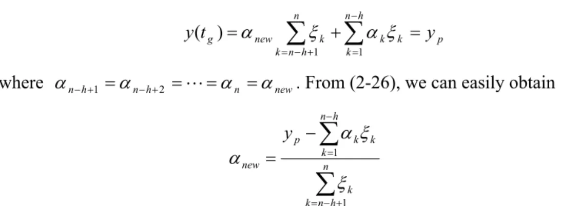
Thus, we have p h n k k k n h n k k new g y t y =

∑

+

∑

− = = + − = 1 1 ) ( α ξ α ξ (2-26) where α_n−h+1 =α_n−h+2 =_L=α_n =α_new. From (2-26), we can easily obtain

∑

∑

+ − = − = − = _n h n k k h n k k k p new y 1 1 ξ ξ α α (2-27)

In this way, not only the bad effect caused by the abrupt variation can be mitigated, but also the future performance of the SFS can be improved by the h new rules.

Remark 2-2: While controlling, a membership function is possible to be pruned if all fuzzy rules associated with this membership function are pruned sequentially.

Remark 2-3: In the implementations of practical systems, if computational burden is the issue having highest priority, the threshold Θ can be chosen large enough so that more fuzzy _p rules are pruned. Hence, the computational burden will be substantially reduced at the expense of less favorable system performance.

Fig. 2-2 shows the flowchart to summarize the self-structuring algorithm for the SFS. The growing and pruning effects during the control period will be illustrated in later sections with excellent result.

p k S <Θ mzx j µ ξ α ˆˆT fc u = σ c αˆ ,ˆ ,ˆ n k S_k , =1 ,2, m j j , 1 ,2, max = µ

2.3 Design of RASFC

Now, we are ready for developing a robust adaptive self-structuring fuzzy controller (RASFC) for the unknown nonaffine nonlinear systems. In the RASFC, an SFS is used to estimate the system uncertainty ∆(x,u) in (2-2). The control law u in the RASFC system is designed as

(

urac ufc

)

z

u= 1 − (2-28) where urac is the robust adaptive controller to achieve a L2 tracking performance with a desired attenuation level and ufc is the self-structuring fuzzy controller to approximate

unknown system dynamics ∆( ux, ). Substituting (2-28) into (2-2) and using (2-4) yield

[

u u u d

]

x e(n) _{= c}(n) _{− rac − fc +∆(x, )+}

[

]

{

u u u u d

}

u x n _{lc fc rac lc} c − − ∆ − + − + = ( ) (_x, ) ( )

[

]

{

u u u u d

}

e _{fc rac lc} T _{− ∆ − + − +} − = k (x, ) ( ) (2-29) or

[

∆ u −u_fc+ u_rac −u_lc +d

]

− =Ae b (x, ) ( ) e& (2-30) where ⎥ ⎥ ⎥ ⎥ ⎦ ⎤ ⎢ ⎢ ⎢ ⎢ ⎣ ⎡ − − − = −1 1 1 0 0 0 0 0 1 0 k k k_{n n L L} L L O O O M L A and _{[00 1]}T K = b 2.3.1 Fuzzy Approximation

The unknown nonlinear function ∆( ux, ) is approximated by an SFS with inputs x and u. In this way, the output of the SFS ufc should be directly fed back to produce u, which is one

of the input of the SFS. This kind of fuzzy system is called a recurrent fuzzy system, as depicted in Fig. 2-3(a). However, a recurrent fuzzy system will lead to a fixed-point problem which must be solved at every time instant and thus imposes computational burden [51, 54-55]. Thus, the following Lemma 2-1 is stated to avoid this problem [51, 54-55].

x

u

Σ

))

,

(

(

u

u

fc

≈

∆

x

rac

u

(a)

x

u

_fc

(

≈

∆

(

x

,

u

))

rac

u

(b)

Fig. 2-3 (a) The recurrent fuzzy system; (b) The static fuzzy system

Lemma 2-1: Let the constant c satisfies the condition ⎟⎟ ⎠ ⎞ ⎜⎜ ⎝ ⎛ ∂ ∂ > u f z 2 1 (2-31) Then, there exist a unique *

fc

u which is a function of x and u so that _rac * ( , )

rac fc u u x satisfies 0 ) , ( ) , , ( ) , , ( * ₌∆_∆ * ₋ * ₌ rac fc fc rac fc rac u u u u u u x x x ψ (2-32)

for all (x,u_rac)∈Ω_x×R.

The Proof of Lemma 1 can be found in [51].

According to Lemma 2-1, the feedback path in Fig. 2-3(a) can be removed. Consequently, a static FS in Fig. 2-3(b) can be used to approximate ∆( ux, ), and thus we do not need to solve the fixed-point problem at every time instant. For the nonaffine systems with the property ∂f x(_∂u,u) <0, Lemma 2-1 can be satisfied as well by simply modifying

(2-31) as _⎟⎟ ⎠ ⎞ ⎜⎜ ⎝ ⎛ ∂ ∂ < u f z 2 1 . Define the vectors c and σ as

T m] [c₁ c₂ c c= _L (2-33) T m] [σ₁σ₂ σ σ= _L (2-34) where [ 1 Nj] j j j= c Lc c and [ 1 Nj] j j j = σ Lσ

Gaussian membership functions of Xj, j=1, 2, …, m, respectively. Rewrite (2-12) in the vector form as ⎥ ⎥ ⎥ ⎥ ⎦ ⎤ ⎢ ⎢ ⎢ ⎢ ⎣ ⎡ = = n n T y ξ ξ ξ α α α M 2 1 2 1 ... ] [ ) , , σc X ( ξ α (2-35) where [ ]T rac u x

X= is the input vector. The output of the SFS used to approximate ∆(x,u) is defined as ξ α σ , c (X ξ αˆT ,ˆ ˆ) ˆTˆ fc u = = (2-36) where αˆ , cˆ , and σˆ are the estimation vectors of α, c, and σ, and ξˆ =ξ(X,cˆ,σˆ). Define the optimal vectors _{α ,} * _{c , and} * _{σ as [3]:} *

⎥⎦ ⎤ ⎢⎣ ⎡ ₋ = × ∈ ∈ ∈ ∈ ) ˆ , ˆ , ˆ , ( ) ( sup min arg ) , , ( ˆ , ˆ , ˆ * * * σ c α X X σ c α x σ c α c Ω σ Ω XΩ Ω α R fc fc u u (2-37) where

{

α

}

α α α Ω = ˆ: ˆ ≤M (2-38) Ω_c =

{

cˆ: cˆ ≤M_c

}

(2-39)

{

σ

}

σ σ σ Ω = ˆ: ˆ ≤M (2-40) andM , _α M , and _c M are positive constants specified by designers. The unknown _σ nonlinear function ∆(x,u) can be described as

∆=_α*T_ξ(X,c*_,σ*₎+ω=_α*T_ξ*+ω (2-41) where _ξ* =_ξ(_X,_c*_,σ*) and ω denotes the approximation error bounded by ω ≤ω , in which ω is a finite positive constant. Then, modeling error u~ can be expressed as

ω + + + = − ∆ = α~ ξˆ αˆ ~ξ α~ ~ξ ~ T T T fc u u (2-42) where α~₌α* ₋αˆ _and ~_{ξ =ξ}* _-ξˆ

. In the following, some preliminaries will be made for adaptive online-tuning of the parameters of fuzzy rules, and thus favorable approximation performance can be achieved in the presence of unexpected disturbances. To achieve this goal, the Taylor linearization technique is employed to transform the nonlinear fuzzy basis function into partially linear form as follows [25, 56]:

o + − ⎥ ⎥ ⎥ ⎥ ⎥ ⎥ ⎥ ⎥ ⎦ ⎤ ⎢ ⎢ ⎢ ⎢ ⎢ ⎢ ⎢ ⎢ ⎣ ⎡ ∂ ∂ ∂ + − ⎥ ⎥ ⎥ ⎥ ⎥ ⎥ ⎥ ⎥ ⎦ ⎤ ⎢ ⎢ ⎢ ⎢ ⎢ ⎢ ⎢ ⎢ ⎣ ⎡ ∂ ∂ ∂ = ⎥ ⎥ ⎥ ⎥ ⎥ ⎦ ⎤ ⎢ ⎢ ⎢ ⎢ ⎢ ⎣ ⎡ = = = ) ˆ ( ) ˆ ( ~ ~ ~ ~ * ˆ 2 1 ˆ 2 1 2 1 σ σ σ σ σ c c c c c ξ σ σ * c c n n n ξ ξ ξ ξ ξ ξ ξ ξ ξ M M M (2-43) or ~ξ =ξT_c~c+ξT_σσ~+o (2-44)

where o represents the higher order term, ~c₌c* ₋cˆ_, ~ =_{σ σ}* _{-σˆ, and}

c c c _{c c c} ξ ˆ 2 1 = ⎥ ⎦ ⎤ ⎢ ⎣ ⎡ ∂ ∂ ∂ ∂ ∂ ∂ = ξ ξ ξn L (2-45) σ σ σ σ σ σ ξ ˆ 2 1 = ⎥ ⎦ ⎤ ⎢ ⎣ ⎡ ∂ ∂ ∂ ∂ ∂ ∂ = ξ ξ ξn L (2-46) Substituting (2-44) into (2-42) yields

ε + + + =α~ ξˆ αˆ ξ_cc~ αˆ ξ_σσ~ ~ T T T T T u ε + + + =α~Tξˆ ~cTξ_cαˆ ~σTξ_σαˆ _(2-47) where αˆTξ_cT~c ₌~cTξ_cαˆand _{ξ σ σ ξ α} σ σ

αˆT T~=~T ˆ since they are scalars, and ε =~αT~ξ+αˆTo+ω is the lumped uncertainty. The higher order term o satisfies

σ ξ c ξ ξ _c~ _σ~ ~ T T o = − + ξ ξc c~ ξσ σ~ ~ ₊ T ₊ T ≤ σ c ~ ~ 2 1 0 b b b + + ≤ (2-48)

where b0, b1, and b2 are bounded positive constants satisfying 0

~ b ≤ ξ , T _≤b₁ c ξ , and 2 b T _≤ σ

ξ . It is reasonable that b0, b1, and b2 exist because Gaussian function and its derivative are always bounded by constants. Moreover, α~, c~, and σ~ satisfy

α α α α α α ˆ ˆ _α ˆ ~ ₌ *_{− ≤} * _{+ ≤M + (2-49)} c c c c c c ˆ ˆ _c ˆ ~ ₌ *_{− ≤} * _{+ ≤M + (2-50)} σ σ σ σ σ σ ˆ ˆ _σ ˆ ~ ₌ * _{− ≤} * _{+ ≤M + (2-51)}

Thus, the lumped uncertainty ε satisfies

ω ε = α~T(ξ_cT~c+ξ_σT~σ+o)+αˆTo+

ω + + + = ~αTξT_c~c α~TξT_σσ~ α*To ) ˆ )( ˆ ( ) ˆ )( ˆ ( ₂ 1 α + α c+ c + α + α σ + σ ≤b M M b M M ω + + + + + +M_α[b₀ b₁(M_c cˆ ) b₂(M_σ σˆ )] T ] ˆ ˆ ˆ ˆ ˆ ˆ ˆ 1 ][ [Λ₁ Λ₂ Λ₃ Λ₄ Λ₅ Λ₆ α c σ α c α σ = Γ ΛT = (2-52) where _{[ ]}T 6 5 4 3 2 1 Λ Λ Λ Λ Λ Λ = Λ , Λ₁ =(b₀ +2b₁M_c+2b₂M_σ)M_α +ω , σ c b M M b_{1 2} 2 = + Λ , Λ₃ =2b₁M_α , Λ₄ =2b₂M_α , Λ₅ =b₁ , Λ₆ =b₂ , and T ] ˆ ˆ ˆ ˆ ˆ ˆ ˆ 1 [ α c σ α c α σ

Γ= . Since Λ is a bounded vector, if Γ is guaranteed to be

bounded, the lumped uncertainty term ε is thus bounded. We can guarantee the boundness of Γ by Lemma 2-2 given in the next subsection.

2.3.2 Parameter Learning Algorithm

Substituting (2-47) into (2-30) yields

)] ( ˆ ~ ˆ ~ ˆ ~ [ T ₊ T ₊ T _{+ +d+ urac −ulc} − =Ae bα ξ c ξ α σ ξ α ε e& _{c σ} . (2-53)

Lemma 2-2 [3]: Suppose that the adaptive laws are chosen as (2-56)-(2-58), where Pr(⋅) is the projection operator, and the symmetric positive P satisfies the following Riccati-like equation 0 1 1 = − + + +PA Q Pb( )b P P A T δ ρ2 T _(2-54)

where Q is a positive definite symmetric matrix and ρ is an attenuation level which satisfies 0

1 1

2 −_δ ≤

ρ . If αˆ(0)∈Ωα, cˆ(0)∈Ωc, and σˆ(0)∈Ωσ, then αˆ t( )∈Ωα, cˆ t( )∈Ωc, and σ

Ω

σˆ t( )∈ for all t≥0 can be guaranteed.

According to Lemma 2-2, Γ in (2-52) is bounded, and hence the lumped uncertainty ε

is bounded. The following theorem shows the properties of the developed control system.

Theorem 2-1: Suppose the assumption (2-3) holds. Consider a SISO nonaffine nonlinear

system (2-1) with the control law (2-28), where the self-structuring fuzzy controller is given as ) ˆ , ˆ , ( ˆ ξ X c σ αT fc u = (2-55)

The adaptive laws are chosen as (2-56)-(2-58): , ) ˆ ( , ˆ ~ ˆ ⎪⎩ ⎪ ⎨ ⎧− = − = ξ Pb e Pr ξ Pb e α α α T T α η η & & ) 0 ˆ ˆ and ˆ ( if ) 0 ˆ ˆ and ˆ ( or ˆ if < = ≥ = < ξ α Pb e α ξ α Pb e α α α α α T T T T M M M (2-56)

where η_α is the positive learning rate and α

α ξ α Pb e ξ Pb e ξ Pb e Pr ˆ ˆ ˆ ˆ ˆ ) ˆ ( ₂ T T T T α α α η η η =− + . ⎪⎩ ⎪ ⎨ ⎧− = − = , ) ˆ ˆ ( , ˆ ˆ ~ ˆ α ξ Pb e Pr α ξ Pb e c c c c T c T c η η & & ) 0 ˆ ˆ and ˆ ( if ) 0 ˆ ˆ and ˆ ( or ˆ if < = ≥ = < α ξ c Pb e c α ξ c Pb e c c c c c c c T T T T M M M (2-57)

where η_c is positive learning rate and c

c α ξ c Pb e α ξ Pb e α ξ Pb e Pr c c c c c c ˆ ˆ ˆ ˆ ˆ ˆ ) ˆ ˆ ( ₂ T T T T _{η η} η =− + . ⎪⎩ ⎪ ⎨ ⎧ − = − = , ) ˆ ˆ ( , ˆ ˆ ~ ˆ α ξ Pb e Pr α ξ Pb e σ σ σ σ σ σ T T η η & & ) 0 ˆ ˆ and ˆ ( if ) 0 ˆ ˆ and ˆ ( or ˆ if < = ≥ = < α ξ σ Pb e σ α ξ σ Pb e σ σ σ σ σ σ σ T T T T M M M (2-58)

where η_σ is positive learning rate and σ

σ α ξ σ Pb e α ξ Pb e α ξ Pb e Pr σ σ σ σ σ σ ˆ ˆ ˆ ˆ ˆ ) ˆ ˆ ( ₂ T T T T _{η η} η =− +

The robust adaptive controller is given as

Pe bT lc rac u u δ 2 1 + = (2-59) Note that since A is designed to be stable in (2-30) and Q in (2-54) is a positive definite symmetric matrix, therefore P must be a positive definite symmetric matrix. Then, the RASFC system can guarantee the global stability and robustness of the closed-loop system and achieve the following L2 criterion [57-58]:

α η 2 ) 0 ( ~ ) 0 ( ~ ) 0 ( ) 0 ( 2 1 2 1 0 α α Pe e Qe e T T T _T dt ≤ +

∫

σ η η 2 ) 0 ( ~ ) 0 ( ~ 2 ) 0 ( ~ ) 0 ( ~_{c c σ} T_σ c T + + +

∫

T +d dt 0 2 2 ) ( 2 ε ρ (2-60) for 0≤ T <∞, where e(0), ~α(0), ~c(0), and σ~(0) are the initial values of e, α~, ,~c and σ~, respectively.

Proof: Define the Lyapunov function candidate as

σ σ c c α α Pe e ~ ~ 2 1 ~ ~ 2 1 ~ ~ 2 1 2 1 T T c T T V σ α η η η + + + = . (2-61)

Differentiating (2-61) with respect to time and using (2-53) yield

σ σ c c α α Pe e e P

e _{& &} & & &

& 1 ~ ~ 1 ~ ~ 1 ~ ~ 2 1 2 1 T T c T T T V σ α η η η + + + + =