國
立
交
通
大
學
資訊科學與工程研究所
碩
士
論
文
可動態重組之材質處理單元
A Run-Time Reconfigurable Texture Unit
研 究 生:汪 威 定
指導教授:鍾 崇 斌 博士
可動態重組之材質處理單元
A Run-Time Reconfigurable Texture Unit
研 究 生:汪 威 定 Student:Wei-Ting Wang
指導教授:鍾 崇 斌 博士 Advisor:Dr. Chung-Ping Chung
國 立 交 通 大 學
資 訊 科 學 與 工 程 研 究 所
碩 士 論 文
A Thesis
Submitted to Institute of Computer Science and Engineering
College of Computer Science
National Chiao Tung University
in Partial Fulfillment of the Requirements
for the Degree of
Master
In
Computer Science
September 2005
Hsinchu, Taiwan, Republic of China
可動態重組之材質處理單元
學生:汪威定 指導教授:鍾崇斌 博士
國立交通大學資訊科學與工程研究所 碩士班
摘 要
材質過濾單元在 3-D 繪圖處理器中佔有相當比重的成本,而且其所佔比例因為以下 兩個原因持續增加中。從 Shader Model 3.0 及 High Dynamic Range 的規格開始支援浮點 格式的材質過濾運算,且 3-D 繪圖處理器架構中的材質過濾單元數量(即材質處理單元 數量,一個材質處理單元包含了一個材質過濾單元和其他元件)也持續增加。故在擬真 畫面的即時顯像下的低成本之材質過濾單元是迫切需要的。材質過濾類別的需求在執行 期間會有所改變,且各種材質過濾類別彼此間具有大量共用的運算,故一個可以彈性地 在各種材質過濾類別做功能切換的材質過濾單元可以大量節省其面積。動態可重組式運 算和 ASIC 相比,提供了一個在較低成本下能得到較高運算速度的機會。此外,需要相 同材質過濾類別需求的連續次數很長也意味著重組代價相對也少。在本篇論文中,我們 提出了一個具低面積速度乘積的可動態重組之材質過濾單元設計。首先,我們針對在單 一材質處理單元內的材質過濾單元提出一個類似 divide-and-conquer 的低面積速度乘積 設計。接著,我們整合多個材質處理單元內的上述材質過濾單元,以組成一個較大並且 跨多個材質處理單元的材質過濾單元,並且設計一套類以 round-robin 的方法提升整合過 後的材質處理單元之使用率。實驗結果顯示此較大並且跨多個材質處理單元的材質過濾 單元相較於多個單一材質處理單元內的材質過濾單元,在僅增加了 2.5%的執行時間下, 節省了 14.2%的面積以及 12.1%的面積速度乘積。
A Run-Time Reconfigurable Texture Unit
Student:Wei-Ting Wang Advisor:Dr, Chung-Ping Chung
Institute of Computer Science and Engineering National Chiao-Tung University
Abstract
Texture filters are one of cost intensive parts in 3-D Graphics Processing Unit architecture and cost of them is increasing due to revealed floating point filtering techniques in Microsoft Shader Model 3.0 with High Dynamic Range feature and increasing number of texture filters (i.e. # of texture unit, a texture unit is composed of a texture filter and other components) required in GPU architecture. Therefore, a low-cost texture filter design in realistic and real-time rendering is required. The usage of filter types varies over run time. Furthermore, there are a large number of shared operations between each filter type. An all-purpose texture filter which can switch flexibly for all filter type can save significant area. Run-time reconfigurable computing offers an opportunity of obtaining high computing speed at lower hardware costs, compared to ASIC. Long run-length of data requiring the same filter type implies small reconfigurable overhead. In this thesis, a run-time reconfigurable texture filter design with low area-time product is proposed. First, a divide-and-conquer-like design for a low area-time product texture filter within a texture unit is proposed. We form a larger texture filter cross multiple texture units to improve its area-time product by integrating the texture filters within multiple texture units, which is the second design. A round-robin-like design to increase the utilization of a reconfigurable texture unit is proposed. The experimental result shows the texture filter cross multiple texture units design achieve 14.2% area saving with 2.5% longer execution time and 12.1% area-time product reduction compared to texture filters within multiple texture units design.
誌 謝
首先感謝我的指導老師 鍾崇斌教授,在老師的諄諄教誨、辛勤指導與勉勵下,我 得以順利完成此論文,並且順利通過畢業口試。同時感謝我的另一位參與計劃老師兼口 試委員 單智君教授以及口試委員 蕭勝夫教授以及 周賜福教授,由於他們的指導與建 議,讓這篇論文更加完整和確實。 此外,感謝實驗室所有同學,尤其是徐日明學長、楊惠親學姊、李元化學長、吳奕 緯學長、蔣昆成學長、喬偉豪學長、林聖勳學長、田濱華學長、黃士嘉學長、葉文涵學 長、鄭式勳學長,以及長期以來合作愉快的陳逸麒,和 GPU 其他組員康哲瑋、張辰瑋、 林慧榛、鍾立傑,給我很多意見和鼓勵。 最後感謝我的家人和朋友,謝謝你們在背後全心全意地支持我,讓我在這研究的路 上走得更順利,進而能無後顧之憂的學習,讓我追求自己的理想。 謹向所有支持我、勉勵我的師長與親友,奉上最誠摯的祝福,謝謝你們。 汪威定 2006. 9. 7Contents
摘 要 ...I ABSTRACT ... II 誌 謝 ... III CONTENTS ...IV LIST OF FIGURES...VI LIST OF TABLES ...VIIICHAPTER 1 INTRODUCTION... 1
CHAPTER 2 BACKGROUND ... 3
-2.1TEXTURE MAPPING...-3-
2.2TEXTURE FILTERING...-4-
2.2.1 Filtering Algorithm ... 4
2.2.2 Weight Generation Algorithm ... 6
-2.3TEXTURE UNIT IN A GPUARCHITECTURE...-8-
2.4TEXTURE FILTER IN A TEXTURE UNIT...-9-
2.5RECONFIGURABLE ARCHITECTURE...-9-
2.6MOTIVATION...-10-
2.7OBJECTIVE... -11-
CHAPTER 3 DESIGN ... 12
-3.1DESIGN ASSUMPTION AND CHALLENGE...-12-
3.2DESIGN OVERVIEW...-12-
3.3SINGLE-BILINEAR ALL-PURPOSE TEXTURE FILTER DESIGN...-13-
3.3.1 Filter Design ... 13
3.3.1.1 Weight Generator and Filter for Linear and Bilinear Filtering Defined in DX9 ... 14
3.3.1.2 Linear Filter Design... 15
3.3.1.3 Bilinear Filter Design ... 16
3.3.1.4 Trilinear and Anisotropic Filter Design ... 17
3.3.2 Additional Filter Logic... 19
3.3.2.1 Additional Filter Datapath ... 19
3.3.2.2 Additional Filter Control ... 21
-3.4MULTI-BILINEAR ALL-PURPOSE TEXTURE FILTER DESIGN...-21-
3.4.2 Fair Fetching and Dispatching Logic Design... 25
3.4.2.1 Priority Sequence Generator Design ... 26
3.4.2.2 Priority Pixel Fetcher Design ... 27
3.4.2.3 Pixel Dispatcher Design ... 28
3.4.3 Choosing the Number of Bilinears as Fundamental Element ... 29
CHAPTER 4 EXPERIMENTAL RESULTS... 33
-4.1GOAL AND METRICS OF THE EXPERIMENTS...-33-
4.2SIMULATION ENVIRONMENTS...-33-
4.3COMPARISONS OF AREA AND CYCLE TIME...-35-
4.4FILTER TYPE STATISTICS OF ALL FILTERING CONFIGURATIONS...-39-
4.5UTILIZATION STATISTICS OF ALL FILTERING CONFIGURATIONS...-41-
4.6COMPARISON OF AVERAGED TOTAL EXECUTION CYCLES AND AREA-TIME PRODUCT...-43-
CHAPTER 5 CONCLUSION AND FUTURE WORK ... 46
-5.1CONCLUSION...-46-
5.2FUTURE WORK...-47-
-List of Figures
Fig. 2-1 Texture Mapping 4
Fig. 2-2 Mipmapping and Filtering Concept 5
Fig. 2-3 Anisotropic Filtering Concept 6
Fig. 2-4 Bilinear Weight Generation Concept 7
Fig. 2-5 Texture Unit in a GPU Architecture 8
Fig. 2-6 Single-Bilinear All-purpose Texture Filter 9 Fig. 3-1 Design Overview of a Two-Bilinear All-Purpose Texture Unit 13 Fig. 3-2 Weight Generation and Filtering for Linear Algorithm 14 Fig. 3-3 Weight Generation and Filtering for Bilinear Algorithm 14
Fig. 3-4 Datapath for Linear Filter 16
Fig. 3-5 Datapath for Bilinear Filter 17
Fig. 3-6 Datapath for Trilinear Filter 18
Fig. 3-7 Datapath for Anisotropic Filter 18
Fig. 3-8 One Bilinear as Fundamental Element 20
Fig. 3-9 Circuit of Additional Filter Control for One Bilinear as Fundamental Element
21
Fig. 3-10 Two Single-Bilinear All-Purpose Texture Units for Two Bi Outputs per Cycle
22
Fig. 3-11 A Multi-Bilinear All-Purpose Texture Unit for One Tri Output or Two Bi Outputs per Cycle
22
Fig. 3-12 Two Bilinears as Fundamental Element 24
Fig. 3-13 Circuit of Additional Filter Control for Two Bilinears as Fundamental Element
Fig. 3-14 Priority Sequence Generator 26
Fig. 3-15 Priority Pixel Fetcher 27
Fig. 3-16 Circuit for Priority Pixel Fetcher 27
Fig. 3-17 Pixel Dispatcher 29
Fig. 3-18 Two Instances of Two Bilinears as Fundamental Element 30 Fig. 3-19 An Instance of Four Bilinears as Fundamental Element 30 Fig. 3-20 Circuit of Priority Pixel Fetcher for Integrating Four Bilinear Filters 31
Fig. 4-1 A frame of DOOM 3 35
Fig. 4-2 Comparisons of Area 36
Fig. 4-3 Comparisons of Cycle Time 38
Fig. 4-4 Filter Type Usages of All Filtering Configurations 39 Fig. 4-5 Numbers of Filter Type Usages of All Filtering Configurations 41 Fig. 4-6 Utilization Statistics for All Filtering Configuration 42 Fig. 4-7 Total Execution Cycles for All Filtering Configurations 43 Fig. 4-8 Comparisons of Averaged Total Execution Cycles 44
List of Tables
Table 2-1 Comparison of bilinear, trilinear, anisotropic filtering algorithms 6 Table 3-1 Comparison of four linear filter designs in terms of area, time and
area-time product
15
Table 3-2 Comparison of two bilinear filter designs in terms of area, time and area-time product
17
Table 3-3 Data flow analysis of all filter type requirements using one bilinear as fundamental element
20
Table 3-4 Data flow analysis of all filter type requirements using two bilinears as fundamental element
23
Table 3-5 Number of required iterations to be iterated for filter type requirement in different fundamental elements
24
Table 3-6 Input-Output mapping for integrating two bilinears 27 Table 3-7 All combinations of two filter type requirements and PF signals for
integrating two bilinears
28
Table 3-8 All combinations of PF signals and pixel dispatch for integrating two bilinears
29
Table 3-9 Comparison for Area of AFL control and Pixel Dispatcher 32 Table 4-1 Area for a single-bilinear all-purpose texture filter 36 Table 4-2 Area for fair fetching and dispatching logic 37 Table 4-3 Area for a multi-bilinear all-purpose texture filter 37 Table 4-4 Filter type usages of all filtering configurations 39 Table 4-5 Numbers of filter type usages of all filtering configurations 40 Table 4-6 Utilization statistics for all filtering configuration 42
Table 4-7 Summary of Comparison for single-bilinear all-purpose design and multi-bilinear all-purpose design
Chapter 1 Introduction
Three-Dimensional (3-D) computer graphics rendering techniques become more complex due to users’ increasing demands for 3-D scene realism improvement [1]. Complex rendering techniques is a computationally intensive task. Computationally intensive task needs high hardware cost. It is challenge to design a low-cost GPU (graphics processing unit) architecture in real-time rendering.
Texture mapping is a technique used to reduce the overall complexity of graphics rendering [2, 3]. It is a technique in which a bit-map called a texture is applied onto an object in the 3D world.
Texture filtering is often necessary for high quality texture mapping. Texture filters are one of cost and computation intensive parts within a texture unit in Graphics Processing Unit (GPU) architecture [4, 5] and cost of them is increasing due to following two reasons:
(1)Floating point filtering techniques revealed in Microsoft SM (Shader Model) 3.0 with HDR (High Dynamic Range) feature increase the cost of texture filter [4];
(2)Increasing # of texture filter (i.e. # of texture unit) [7, 8] is required in conventional GPU architecture [8];
To reduce cost of texture filters is an important issue.
Filter type requirement varies in run-time. Single-purpose texture filter may be idle in run-time. Furthermore, there are a large number of shared operations between each filter type. We can use an all-purpose reconfigurable texture filter to flexibly switch among all filter types.
Reconfigurable computing offers an opportunity for obtaining high computing speed at lower hardware costs, compared to ASIC [9]. The principal difference when compared to
ASIC is the ability to make substantial changes to the data path itself in addition to the control flow.
We propose a run-time reconfigurable texture unit, which can be divided into inside-texture filter and outside-texture filter since a texture unit is composed of a texture filter, an address generator, and a texture cache. The reconfiguration of our proposed texture unit architecture is composed of inside-texture filter reconfiguration and outside-texture filter (inside-texture unit) reconfiguration.
For inside-texture filter part, we propose a divide-and-conquer-like method to design low-area-time product texture filters for all texture filtering algorithms used in current 3D games. Then, we use all types of low-area-time product texture filters and a given fundamental element to design a single-fundamental element all-purpose texture filter.
Although reconfigurable computing provides flexibility for many different applications, it causes reconfigurable overhead while changing configurations for different applications. We observe over 93% of the total filtered pixels are in 31% runs which have more than 2000 length. Each run of data has the same filter type. There is low reconfigurable overhead for outside-texture filter due to long run-length of data requiring the same filter type.
We integrate above texture filters within multiple texture units to form a larger texture filter cross texture units in outside-texture filter part. A round-robin-like method to maximize the utilization of texture filter cross texture units is presented.
The reminder of this paper is organized as follows: Section 2 introduces background of algorithm and architecture of texture mapping and texture filtering. Section 3 describes our proposed reconfigurable texture unit including inside-texture-filter reconfiguration and outside-texture-filter reconfiguration. The experimental results and analysis are described in section 4. Conclusions and future works are made in section 5.
Chapter 2 Background
In this chapter, we will give an overview of texture mapping and texture filtering. Then, two processes of texture filtering algorithm called weight generation algorithm and filtering algorithm will be introduced. We will focus on texture filtering algorithm used in current 3D games. Finally, we present the conventional texture unit design, especially on texture filter part.
2.1 Texture Mapping
Texture mapping is a relatively efficient means to reduce computations for a realistic scene without the tedium of modeling and rendering every 3-D detail of a surface [2, 3]. It is a process in which a 2D bit-map mage called a texture is applied to an object in the 3D world, as shown in Fig. 2-1. x and y are pixel coordinates. S and t are texel (texture element) coordinates.
The number of required triangles is increased and thus the number of calculations is increased due to realize realistic images or a very complex image. The number of polygons should be reduced because the computing power of the given system is not enough to perform the required calculations in time. So quality degradation in terms of scene complexity is introduced but in some cases this degradation is not tolerable. Hence, to have more realistic images with less geometric data, texture mapping has been used commonly in 3D computer graphics.
x y
s t
Pixels in screen Texels in texture s
t s t
Pixels in screen Texels in texture Fig. 2-1. Texture Mapping
2.2 Texture Filtering
Due to the absence of no one-to-one mapping between texels and pixels, an interpolation calculation is necessary for high quality mapping. Higher quality requires computation intensive interpolation to generate a final pixel value from many texel values.
Commonly used texture filtering algorithms in current 3D games are bilinear (Bi), trilinear (Tri), anisotropic (Ani). There is a tradeoff between operation complexity and image quality among various texture filtering algorithms. 1-D Linear (Li) filtering algorithm will be introduced since all filtering algorithms are based on Linear. Texture filtering process is composed of filtering and weight generation. We will introduce both filtering and weight generation algorithms for linear, bilinear, trilinear and anisotropic filtering.
2.2.1 Filtering Algorithm
Filtering algorithm includes linear, bilinear, trilinear and anisotropic. Both trilinear and anisotropic support mipmapping technique. Mipmapping is a technique to reduce the artifacts which arise from the use of a single bitmap image while the level of detail of an object decreases with an increase in the distance. It is made by an original-size texture with level-of-detail 0 (LOD 0), then iteratively resample it to make a half-size texture with LOD i (i>1). The number i depends on application designer. In figure 2-2, there are three LODs for
mipmapping. The original-size texture (LOD 0) is 8x8, LOD 1 is 4x4, and LOD 2 is 2x2.
Fig. 2-2. Mipmapping and Filtering Concept
The final value of linear filtering is a weighted average of two values. The final value of bilinear is to return the weighted average of the four texels that are closest to the center of the pixel being textured. Trilinear is to choose the two mipmaps that most closely match the size of the pixel being textured and use bilinear filter to produce a texture value from each mipmap. In the example of Fig 2-2, two mipmaps are LOD0 and LOD1, respectively. The final texture value is a weighted average of those two values according to the value of LOD.
If we need to do texture mapping for a plane which is at an oblique angle to the camera, traditional isotropic filters (bilinear/trilinear) would give us insufficient horizontal resolution and extraneous vertical resolution. Anisotropic is a method of enhancing the image quality of textures on surfaces that are far away and steeply angled with respect to the camera. The final texture value of n:1 anisotropic is an average of the values of n trilinears results. The value n called anisotropic ratio, the ratio of horizontal direction to vertical direction, is defined by game designer. The value may be 2, 4, 8, or 16. In Fig 2-3, we use n=2 as an example. The comparison of bilinear, trilinear, and anisotropic filtering algorithms is shown as table 2-1. The equations of above three filter types are equation 1, equation 2, and equation 3, respectively.
Fig. 2-3. Anisotropic Filtering Concept Filtering Type # of MipMap # of Texel / MipMap # of Texel (# of Bi) Filtering Algorithm Bi 1 4 4 (1) (1) Tri 2 4 8 (2) (2) n:1 Ani n=2,4,8,16 2 4n 8n (2n) (3) Table 2-1. Comparison of bilinear, trilinear, anisotropic filtering algorithms
2.2.2 Weight Generation Algorithm
values. For example, using one fraction of coordinates (FC) input called LOD to generate two weight outputs for interpolating two bilinear results. Weight generation algorithm for Linear is shown as equation 4, where FC denotes fraction of coordinate.
(4)
Bilinear weight generation algorithm is used for interpolating four texels of a bilinear. As shown in Fig. 2-4, a texture coordinate is composed of integer part and fractional part. Using two FC inputs called fraction of X coordinate and fraction of Y coordinate to generate four weight outputs for four texels of a bilinear. Equation 5 is weight generation algorithm for Bilinear.
Fig. 2-4. Bilinear Weight Generation Concept
(5)
algorithms and one linear weight generation algorithm. A n:1 Anisotropic weight generation algorithm is composed of n*2 trilinear weight generation algorithm and used for averaging n trilinear results. Using an anisotropic ratio (AR=n) input to generate n weight outputs which have the same weight value (1/n).
2.3 Texture Unit in a GPU Architecture
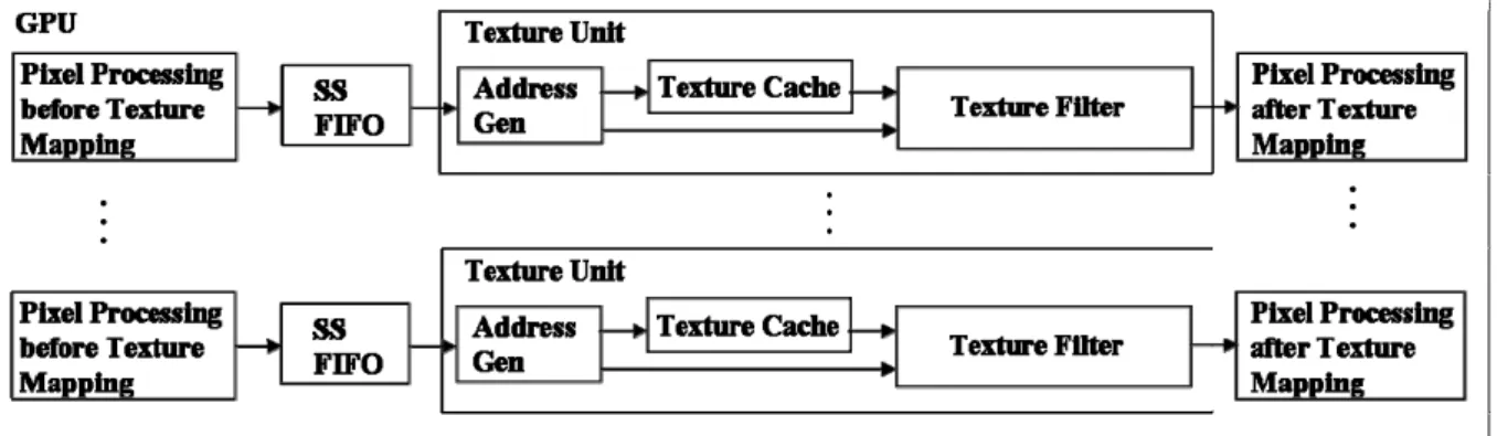
There are multiple texture units in a reference GPU and each of them has a texture filter [7, 8]. Texture unit supports texture mapping operation mentioned in section 2-1. Each texture unit is composed of an address generator, a texture cache, and a texture filter, as shown in figure 2-5. Sampler states (SS) define texture sampling operations such as texture addressing and texture filtering [4]. We concentrate on filter type and anisotropic ratio requirement of a pixel to be filtered since we only focus on texture filter design. Input data of each texture unit is from its (SS) FIFO. Then, address generator transforms texture coordinate to cache address for cache accessing. On the other hand, address generator pass the fractional part of texture coordinate and LOD value to texture filter. After receiving texels from texture cache and weights from address generator, texture filter generates filtered pixel according to filter type and anisotropic ratio.
2.4 Texture Filter in a Texture Unit
We define a texture filter composed of a bilinear filter and additional filter logic (for supporting trilinear and anisotropic filtering) as a Single-Bilinear All-Purpose (SBAP) texture filter, as shown in figure 2-6 [4, 5]. Bilinear filter is a logic with function of bilinear filtering algorithms mentioned before. Additional filter logic for bilinear (AFL_Bi) denotes using bilinear as fundamental element. An additional filter logic is composed of additional filter datapath and additional filter control. Additional filter datapath iteratively cooperates with the bilinear filter to do trilinear or anisotropic filtering. Additional filter control generates the number of iteration to accomplish trilinear or anisotropic filtering.
The throughput of Single-Bilinear All-Purpose texture filter is one bilinear output per cycle and one Tri output every two cycles [4, 5]. In the column “# of texel (# of Bi)” of table 2-1, we define trilinear in terms of 2 bilinears and anisotropic in terms of 2n bilinears since fundamental element is bilinear.
Fig. 2-6. Single-Bilinear All-purpose Texture Filter
2.5 Reconfigurable Architecture
A reconfigurable architecture can be classified as fine-grained and coarse-grained according to the granularity of the fundamental element. Fine-grained architecture, such as a field programmable gate array (FPGA) [10-12], has higher flexibility but lower execution
performance compared with a coarse-grained architecture. A coarse-grained architecture has fundamental elements with higher computing capacity and less routing requirements; hence it may significantly reduce the silicon areas [13].
However, the development of the compiler supporting the architecture has been very difficult because of the complex computation and various execution time [14]. The purpose of this study was to develop an efficient method to eliminate the waste of resources cause by idle fundamental elements. We adopt coarse-grained architecture due to following two reasons:
(1) Timing issue is one of important concerns for a GPU;
(2) The flexibility for limited numbers of filter type combinations is low.
Applications that can be accelerated through the use of reconfigurable hardware are too many to be loaded simultaneously onto the available hardware. Run-time reconfigurable architecture is used to solve the problem. It is able to swap different configurations in and out of the reconfigurable hardware during run-time. Therefore, our proposed design is a run-time reconfigurable architecture.
2.6 Motivation
Area of texture filter need to be improved due to texture filters are one of cost intensive parts in GPU architecture and cost of them is increasing. Moreover, area of additional filter logic need to be improved due to additional filter datapath occupies a large portion of cost in a texture filter. Besides, reconfigurable architecture is adopted due to the following three reasons:
(1) Single-purpose texture filter may be idle due to filter type requirement varies in run-time;
(2) A large number of shared logic saves area for an all-purpose texture filter due to a large number of similar operations between each filter type;
(3) Less reconfigurable overhead due to long run-length of data requiring the same filter type; we observe that over 93% of the total filtered pixels are in 31% runs which have more than 2000 length, where each run of data has the same filter type.
2.7 Objective
For texture filtering algorithms used in current 3D games, we provide low-area-time product necessary function called Bi filter and low-area-time product AFL and achieve low area-time product (AT) texture filter design.
Chapter 3 Design
In this chapter, we first describe design assumption and challenges for designing a reconfigurable texture filter. Then, a brief design overview is present. Our design is composed of two parts:
(1) Single-bilinear all-purpose texture filter design, which is composed of filter design and implementing additional filter logic according to our filter design;
(2) To save area of AFL, we propose a multi-bilinear all-purpose texture filter design, which is composed fair fetch and forwarding logic design and to choose proper number of bilinear filters to be integrated.
3.1 Design Assumption and Challenge
The only one design assumption is using 16-bit floating point (s5.10) format as default operation widths. It refers to Microsoft Shader Model (SM) 3.0 with High Dynamic Range (HDR) feature. There are two design Challenges. How to design Bi filter for low AT and implement additional filter logic for low AT using low AT Tri/Ani filters for single-bilinear all-purpose texture filter design. The other is what number of Bi texture filters should be integrated for multi-bilinear all-purpose texture filter design. There is a trade off between area saving of AFL and overhead of fair fetching and forwarding logic.
3.2 Design Overview
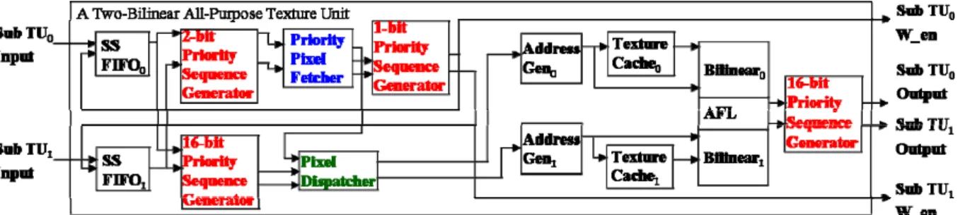
There main components in MBAP TU are filter design, additional filter logic, fair fetching and forwarding logic. Figure 3-1 is a MBAP TU with integrating two SBAP TUs.
Fair fetching and forwarding logic are all necessary logics to maximize utilization of reconfigurable TU. It includes priority sequence generator, priority pixel fetcher, and pixel dispatcher.
Fig. 3-1. Design Overview of a Two-Bilinear All-Purpose Texture Unit
3.3 Single-bilinear All-purpose Texture Filter Design
Before designing a multi-bilinear all-purpose texture filter, we design a single-bilinear all-purpose texture filter design. it is composed of filter design and additional filter logic design.
3.3.1 Filter Design
The goal of filter design is implementing a single-bilinear all-purpose texture filter. We use a Divide-and-Conquer-like method. It works by recursively breaking down a problem into two or more sub-problems of the same type, until these become simple enough to be solved directly. The solutions to the sub-problems are then combined to give a solution to the original problem. For filter design, we define linear as sub-problem and filter types with more computation requirement (Bi/Tri/Ani) as the original problem. First, we find minimum-AT Li filter using brute force method. Then, we implement Bi/Tri/Ani filters using minimum-AT Li filters to approach minimum-AT Bi/Tri/Ani filter design.
3.3.1.1 Weight Generator and Filter for Linear and Bilinear
Filtering Defined in DX9
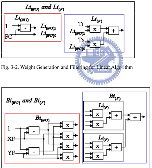
According to weight generation and filtering algorithm mentioned in section 2, weight generator (WG) and filter (F) for linear and bilinear filtering algorithms defined in DX9 is shown in figure 3-2 and figure 3-3, respectively.
Fig. 3-2. Weight Generation and Filtering for Linear Algorithm
3.3.1.2 Linear Filter Design
There are three possible equation arrangements for linear texture filtering algorithm. Equation 6 denotes an original form combining linear weight generation and filtering algorithm. Equation 7, 8 and 9 are other three rearranged equations.
(6)
(7)
(8)
(9)
Table 3-1 shows comparison of above four linear filtering algorithm in terms of area and time. The linear filter according to equation 9 has minimum area and the same time as other to equations. Hence, we adopt equation 9 which has minimum-area-time product as our linear filtering algorithm and its corresponding design is shown as figure 3-4.
Eq. Area (um^2) Time (ns) AT
(6) 66927.171875 11.88 795094.801875
(7) 66710.953125 12.36 824547.380625
(8) 49812.839844 11.92 593769.05094048
(9) 50468.140625 11.66 588458.5196875
Fig. 3-4. Datapath for Linear Filter
3.3.1.3 Bilinear Filter Design
There are too many possible equation arrangements for bilinear texture filtering algorithm. We define bilinear filtering algorithm as original problem and divide it into many sub-problem called linear filtering algorithm. The first line of equation set 10 denotes an original form combining bilinear weight generation and filtering algorithm. The last line of Equation set 10 is one of rearranged equation. We use two equation 9 to replace two linear filtering algorithm in above equation to generate equation 11. We use another linear filtering algorithm to replace equation 9 since equation 11 has the same form as equation 9. The result of bilinear filter design, composed of three linear filter, is shown as figure 3.5.
(10)
Fig. 3-5. Datapath for Bilinear Filter
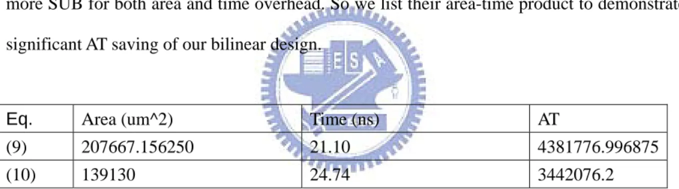
From table 3-2 we observe that equation 9 has area saving of 5 MULs. But it needs 1 more SUB for both area and time overhead. So we list their area-time product to demonstrate significant AT saving of our bilinear design.
Eq. Area (um^2) Time (ns) AT
(9) 207667.156250 21.10 4381776.996875
(10) 139130 24.74 3442076.2
Table 3-2. Comparison of two bilinear filter designs in terms of area, time and area-time product
3.3.1.4 Trilinear and Anisotropic Filter Design
We use the same divide-and-conquer-like method to divide trilinear filtering algorithm into multiple bilinear and linear filtering algorithm. The last line of equation set 12 shows a trilinear filter is composed of two bilinear filters and one linear filter (i.e; seven linear filters). The datapath of above trilinear design is shown as figure 3-6.
(12)
Fig. 3-6. Datapath for Trilinear Filter
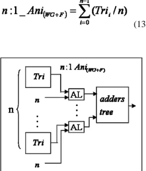
Equation 13 shows a n:1 anisotropic filtering algorithm is summation of n trilinear results dividing n. The datapath of a n:1 anisotropic filter is shown as figure 3-7. the anisotropic logic (AL) provide a division for n, which is a subtraction from exponent part.
(13)
3.3.2 Additional Filter Logic
The goal of additional filter logic is to implement additional filter datapath and control for low AT. We define n bilinears as a fundamental element at design time, where n equals to the number of integrated Bi texture filters. The requirement analysis is composed of case of multiple outputs in single-cycle and case of single output in multi-cycle.
For the case of multiple outputs in single-cycle, if the datapath of fundamental element can execute more than one computations of current filter type requirement in one-cycle, we divide the datapath of fundamental element into multiple current filter type requirements. For example, we divide a trilinear of fundamental element into 2 bilinears of current filter type requirements.
For the case of single output in multi-cycle, if the datapath of fundamental element needs to execute the current filter type requirement in multi-cycle, we divide current filter type requirement (m*n bilinears) into m fundamental requirements (n biliears). Then, we use a fundamental element and an additional filter datapath for m iterations to achieve current filter type requirement. For example, we divide a k:1 anisotropic of current filter type requirement into k trilinears of fundamental requirements.
3.3.2.1 Additional Filter Datapath
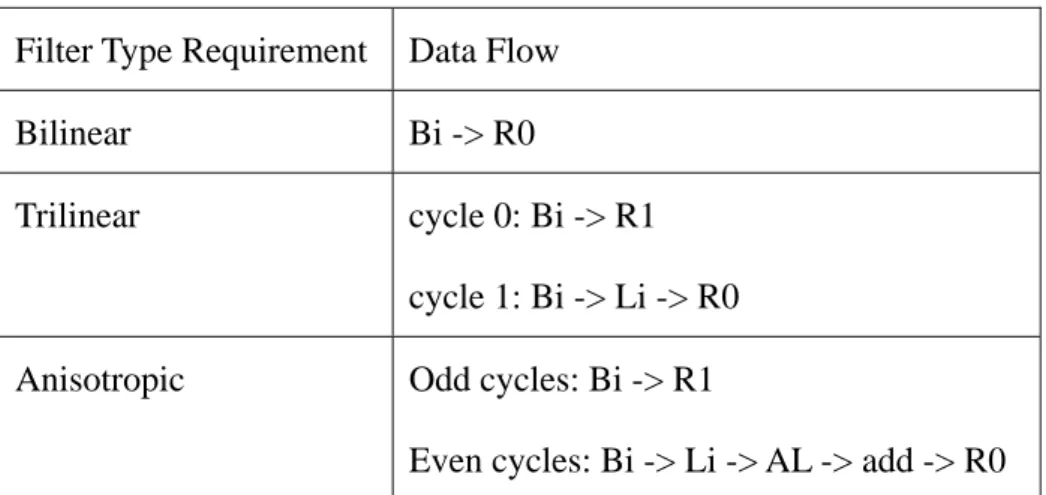
Table 3-3 shows data flow analysis of all filter type requirements for one bilinear as fundamental element. The component of data flow is derived from trilinear datapath and anisotropic datapath shown in figure 3-6 and figure 3-7.
Filter Type Requirement Data Flow Bilinear Bi -> R0
Trilinear cycle 0: Bi -> R1 cycle 1: Bi -> Li -> R0 Anisotropic Odd cycles: Bi -> R1
Even cycles: Bi -> Li -> AL -> add -> R0
Table 3-3. Data flow analysis of all filter type requirements using one bilinear as fundamental element
Figure 3-8 shows an one bilinear as fundamental element derived from table 3-3. To achieve a trilinear output every two cycles, we need a extra linear filter. To achieve a n:1 anisotropic output every 2n cycles, we need an extra 16-bit register R1 to save trilinear results, an extra anisotropic logic to divide each trilinear result and an adder to accumulate all trilinear results. 16-bit register R0 is not included in additional filter datapath due to it is a necessary pipelined register if we consider a texture filter as a pipe stage in GPU. We use two bits to represent filter type (FT) requirement. 00 represents bilinear, 01 represents trilinear, and 10 represents anisotropic. MUX 0 is to distinguish if the filter type requirement is bilinear. MUX 1 is to distinguish if the filter type requirement is trilinear. A 1-bit register with an inverter is used to represent odd and even cycles.
3.3.2.2 Additional Filter Control
The number of required iterations is different for all filter type requirement. A trilinear and a n:1 anisotropic requirements need 2 and 2*n iterations using a bilinear as fundamental element. The counter size represents maximum width to iterate 16:1 anisotropic, which is log2(16*2)-bit.
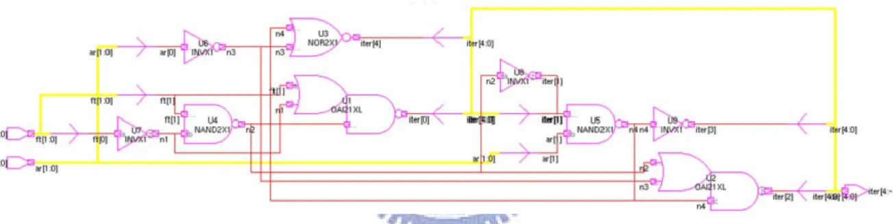
. A tool can draw and display schematics of the synthesized designs called design_vision. We use it to produce circuits of additional filter control for one bilinear as fundamental element, as shown in figure 3-9.
Fig. 3-9. Circuit of Additional Filter Control for One Bilinear as Fundamental Element
3.4 Multi-bilinear All-purpose Texture Filter Design
The additional filter logic and fair fetching and dispatching logic for multi-bilinear all-purpose texture filter will be proposed in this section. Since each single-bilinear all purpose texture filter needs a additional control logic, we can design a multi-bilinear all purpose texture filter to shared only one additional control logic with lower area than a additional control logic using one bilinear as fundamental element. We use a example to compare two instances of single-bilinear all-purpose texture filter and a two-bilinear all-purpose texture filter, as shown in figure 3-10 and 3-11, respectively. Fair fetching and
dispatching logic is to maximize the utilization of multi-bilinear all-purpose texture unit due to properly allocating the requirement to all address generators.
Fig. 3-10. Two Single-Bilinear All-Purpose Texture Units for Two Bi Outputs per Cycle
Fig. 3-11. A Multi-Bilinear All-Purpose Texture Unit for One Tri Output or Two Bi Outputs per Cycle
3.4.1 Additional Filter Logic for Multi-bilinear All-purpose
Texture Filter
For the additional filter datapath, table 3-4 shows data flow analysis of all filter type requirements for two bilinear as fundamental element. The component of data flow is derived from trilinear datapath and anisotropic datapath shown in figure 3-6 and figure 3-7.
Filter Type Requirement Data Flow
Bilinear Bi0 -> R0 or Bi1 -> R1 Trilinear Bi -> Li -> R0
Anisotropic Each cycle: Bi -> Li -> AL -> add -> R0
Table 3-4. Data flow analysis of all filter type requirements using two bilinears as fundamental element
Figure 3-12 shows two bilinears as fundamental element derived from table 3-3. we remain the same throughput, two bilinear outputs per cycle, as the design of two instances of one bilinear as fundamental element. We need an extra linear filter to achieve a trilinear output. To achieve a n:1 anisotropic output every n cycles, we need an extra anisotropic logic to divide each trilinear result and an adder to accumulate all trilinear results. The design of two bilinears as fundamental element keeps the same throughput and save an additional datapath for one bilinear compared to the design of two instances of one bilinear as fundamental element.
Fig. 3-12. Two Bilinears as Fundamental Element
For the additional filter control, the number of required iterations for the combination of all kinds of fundamental element and all filter type requirement is shown as table 3-5. The circuits of additional filter control using two bilinear as fundamental element, as shown in figure 3-13. Comparing to using one bilinear as fundamental element, the fundamental element with more number of bilinears needs less additional filter control overhead for both area and time.
Fundamental Element \ Filter Type Requirement
Bi Tri m:1 Ani Counter size (bit)
1 Bi 1 2 m*2 log2(16*2)
2 Bis (Tri) 1 1 m log2(16)
2n Bis (n:1 Ani) 1 1 m/n log2(16)-log2(n)
Table 3-5. Number of required iterations to be iterated for filter type requirement in different fundamental elements
Fig. 3-13. Circuit of Additional Filter Control for Two Bilinears as Fundamental Element
3.4.2 Fair Fetching and Dispatching Logic Design
The fair fetching and dispatching logic is a round-robin-like method to maximize utilization of multi-bilinear all-purpose texture unit. Round-robin is an arrangement of choosing all elements in a group equally in some rational order. The fair fetching and dispatching logic is composed of priority sequence generators, priority pixel fetcher, and pixel dispatcher mentioned in figure 3-1 before.
Fair fetching avoids load-imbalanced sampler states FIFOs. Empty FIFO may cause utilization loss. Priority sequence generator switches the n different priority sequences of fetching and filtering pixels for n FIFOs every n cycles. Priority pixel fetcher logic determines which pixels can be fetched and filtered in this cycle according to the above priority sequences and the limitation of filter width. To flexibly utilize resources in texture unit, we propose a pixel dispatcher logic to dispatch m (ranged from 1 to n) pixel requirements to n address generators (AGs) since it may allocate more than 1 AG for 1 pixel requirement in a cycle.
3.4.2.1 Priority Sequence Generator Design
The function of priority sequence generator is to switch the n different priority sequences of fetching and filtering pixels for all FIFOs every n cycle. The value n is the number of pixel requirement (the number of integrated Bi texture filters). The priority sequence generator inputs n pixel requirements and outputs n priority sequences. It is composed of two components. n n-to-1 MUXs represent all Input-Output-Mappings. A log2n-bit counter switches the n different Input-Output-Mappings every n cycle.
Figure 3-14 is an example using n=2. Table 3-6 shows two priority sequences for odd cycles and even cycles. A 1-bit register with an inverter is used to represent odd and even cycles. The width of priority sequence generator may be 1, 2, 16 bits according to data width. In figure 3-1, the two priority sequence generators directly connected to FIFO generate priority sequence from two sources (pixels from two FIFOs). 16-bit priority sequence generator processes pixel data. 2-bit priority sequence generator processes filter type data. The other two priority sequence generators recover the priority sequence to original sequence (from FIFO 0 to FIFO 1). The 1-bit priority sequence generator process the signals for pixels can be fetched and filtered in this cycle. The 16-bit priority sequence generator process the pixel data to destination registers.
Case O0 O1
0 I 0 I 1
1 I 1 I 0
Table 3-6. Input-Output mapping for integrating two bilinears
3.4.2.2 Priority Pixel Fetcher Design
Priority pixel fetcher determines which pixels can be fetched and filtered in this cycle by according to the priority sequences and checking the limitation of filter width. The priority pixel fetcher inputs n filter type of pixels (FT) and an anisotropic ratio of all pixels (AR) and outputs n Boolean value of pixel of each FIFO whether can be fetched and filtered or not in this cycle (PF). The value n is the number of pixel requirement (the number of integrated Bi texture filters). Figure 3-15 shows a priority pixel fetcher using n=2 as an example. Lower index i of input pixel denote higher priority to be fetched and filtered. Hence, FT0 has highest priority. The circuit of a priority pixel fetcher using n=2 is shown as figure 3-16.
Fig. 3-15. Priority Pixel Fetcher
The utilization effected by different combinations of filter type requirements is discussed as follows: Table 3-7 lists all combinations of two filter type requirements and PF signals for integrating two bilinears. “none” in column “FT i” means FIFO i is empty.
Case 0, 1, and 2 have no effects on utilization for both single-bilinear all-purpose design and design of integrating two bilinears. We define case 3 and 4 as utilization loss due to empty FIFO. The one bilinear utilization loss results from one FIFO is empty and the other one filter type requirement is bilinear. Both two designs have these cases. Case 5 and 6 are utilization gain due to integrating multiple bilinear texture filters. The utilization gain of 1 bilinear due to the idle bilinear filter can be utilized for trilinear or anisotropic filtering. Utilization loss due to integrating multiple Bi texture filters are case 7. The utilization loss of 1 bilinear due to the additional filter logic using two bilinears as fundamental element only supports looping based on trilinear. Case FT 0 FT 1 PF 0 PF 1 0 Bi Bi 1 1 1 Tri Bi/Tri/Ani 1 0 2 Ani Bi/Tri/Ani 1 0 3 Bi none 1 0 4 none Bi 0 1 5* Tri/Ani none 1 0 6* none Tri/Ani 0 1 7* Bi Tri/Ani 1 0
Table 3-7. All combinations of two filter type requirements and PF signals for integrating two bilinears
3.4.2.3 Pixel Dispatcher Design
PF signals, as shown in figure 3-17. The value n is the same as former definition. We assume that while using two neighboring bilinear filter 0 and bilinear filter 1 to do trilinear or anisotropic filtering, bilinear filter 0 and bilinear filter 1 process the odd/even and even/odd LOD levels in odd/even cycles, respectively. Therefore, these two bilinear filter cooperate a trilinear or anisotropic filtering. Pixel dispatcher inputs pixels from their corresponding FIFOs and outputs pixels to n AGs.
Fig. 3-17. Pixel Dispatcher
In table 3-8, case 0 represents AG 0 and AG 1 are used for their corresponding Bi filtering. Case 1 represents both two AGs are used for FT0 filtering. Case 2 represents both two AGs are used for FT1 filtering.
Case PF 0 PF 1 AG 0 AG 1
0 1 1 Bi 0 Bi 1
1 1 0 FT 0 FT 0
2 0 1 FT 1 FT 1
Table 3-8. All combinations of PF signals and pixel dispatch for integrating two bilinears
3.4.3 Choosing the Number of Bilinears as Fundamental Element
Compared to integrating two bilinear filters, integrating more than two of them is insufficient with both area and time. We will analyze both the additional filter logic and fairfetching and dispatching logic.
For additional filter datapath part, integrating more than two bilienars (n>2) needs extra ((log2n)-1) floating-point adder time delay with no area saving. Figure 3-18 and 3-19 shows
the additional datapath of case n=2 and n=4, respectively. The design of n=4 has an extra floating-point adder delay.
Fig. 3-18. Two Instances of Two Bilinears as Fundamental Element
For additional filter datapath part, integrating more than two bilienars (n>2) needs an extra additional filter control for n bilinears (except for n=32, which can perform any filter type requirement in one cycle) but saves (n/2) additional filter control for 2 bilinears.
For fair fetching and dispatching logic, we divide it into three parts. Priority Pixel Fetcher has more complex mapping logic due to more cases. Figure 3-20 shows a circuit of priority pixel fetcher for integrating four bilinear filters, which is more complex than circuit of priority pixel fetcher for integrating two bilinear filters in figure 3-16.
Fig. 3-20. Circuit of Priority Pixel Fetcher for Integrating Four Bilinear Filters
The components of pixel dispatcher change from n 2-to-1 MUX to n n-to-1 MUX. The components of priority sequence generator change from n*2 2-to-1 MUXs to n*2 n-to-1 MUXs. Moreover, worst case of utilization loss due to integrating multiple bilinears also changes from one bilinear to n-1 bilinears.
can show the fact that both area and time overhead for case n>2 are both larger than case n=2. We only compare their area since time overhead of case n>2 larger than case n=2 for both additional filter logic and fair fetching and dispatching logic. Table 3-9 shows the rapidly increasing area overhead for only pixel dispatcher part is much larger than area saving for additional filter control while increasing number of integrated bilinears.
Area (um^2) AFL control Pixel Dispatcher Total
N=2 18202.06128 40874.804672 59076.865952 (100%) N=4 7291.468872 122624.414016 129915.882888 (220%) N=8 2341.785612 286123.632704 288465.418316 (488%) N=16 472.348794 613122.07008 613594.418874 (1039%) N=32 0 1267118.944832 1267118.944832 (2145%) Table 3-9. Comparison for Area of AFL control and Pixel Dispatcher
Chapter 4 Experimental Results
In this chapter, we first show the goal and metrics of the experiments. Then, simulation environment is introduced. Thirdly, we compare and discuss the comparison of area, cycle time, and total execution cycles. We will analyze the result of total execution cycles according to filter type statistics and utilization statistics of all filtering configurations. Last but not least, the comparison of area-time product is presented.
4.1 Goal and Metrics of the Experiments
Experiment goal is to compare single-bilinear all-purpose design (two TUs for two Bi outputs per cycle) and two-bilinear all-purpose design (one TU for one Tri output or two Bi outputs per cycle). We use two-bilinear all-purpose, which is the lowest area-time product design of all possible number of bilinear filters to be integrated to denote multi-bilinear all-purpose design in this section.
Experiment metrics is area-time product (AT). It is composed of product of area and time. Time is composed of cycle time and total execution cycles. The area and cycle time is gathered from hardware synthesis. The total execution cycles is gathered from software simulation.
4.2 Simulation Environments
Simulation environment is composed of hardware synthesis environment and software simulation environment. We introduce hardware synthesis environment first. Verilog HDL
was adopted as the high-level language for implementing the texture unit design. Verilog HDL codes were written to describe the architecture and behavior of each component. The entire architecture was tested for functional correctness using the C language. After the function of the design had been tested successfully with the Altera Quartus two functional simulator, the design is synthesized by Synopsys design compiler with TSMC 0.18um process.
Software simulation environment is a trace-driven C++ simulator for texture unit architecture. We assume no cache miss and infinite SS FIFO size and use 16 texture units and each of them has a bilinear filter (the same as NVIDIA GeForce 6800). The benchmark is a modern graphic application called DOOM 3, as shown in figure 4-1. The simulator inputs trace of benchmark from modified DirectX 9 reference rasterizer and outputs total execution cycles. The trace contains pixels to be filtered with information of filter type and anisotropic ratio. And DirectX 9 reference rasterizer is a software device that implements the entire Direct3D feature set.
Fig. 4-1. A frame of DOOM 3
4.3 Comparisons of Area and Cycle Time
The comparison of area is shown as figure 4-2. Area of each component in single-bilinear all-purpose design is listed in table 4-1. The area of a single-bilinear all-purpose design should be multiplied by two to compare with multi-bilinear all-purpose design. Therefore, total area is405695.6628 (=202847.8314 * 2).
3245565.302 2785234.619 2500000 2600000 2700000 2800000 2900000 3000000 3100000 3200000 3300000 SBAP MBAP Design Ar ea ( um ^2 )
Fig. 4-2. Comparisons of Area
Component Area (um^2)
fpADD 14599.56836 AL 1081.079956 Bilinear 133132.5156 Ctrl_Bi 1397.712036 Linear 47873.55078 MUX16b2to1_0 565.487976 MUX16b2to1_1 898.127991 REG1b 126.403198 REG16b 1357.171143 REG16bWen 1816.214355 Total_ SBAP_TF 202847.8314
Table 4-1. Area for a single-bilinear all-purpose texture filter
dispatching logic and a multi-bilinear all-purpose texture filter. Area of each component in fair fetching and dispatching logic and multi-bilinear all-purpose texture filter are listed in table 4-2 and table 4-3, respectively. Therefore, total area is 349574.700193 (=6439.910293 + 343134.7899). The area of fair fetching and dispatching logic called reconfigurable area overhead occupies only 2% of total area since floating-point operations in multi-bilinear all-purpose texture filter is very area-intensive.
Component Area (um^2)
PrioritySequenceGenerator1b2to1 73.180801 PrioritySequenceGenerator2b2to1 332.640015 PrioritySequenceGenerator16b2to1_0 2268.604736 PixelDispatcher 1916.006348 PriorityPixelFetch 206.236816 PrioritySequenceGenerator16b2to1_1 1643.241577 Total_FFDL 6439.910293
Table 4-2. Area for fair fetching and dispatching logic
Component Area (um^2)
fpADD 14589.589844 AL 1184.198242 Bilinear_0 133874.296875 Bilinear_1 139130 Ctrl_Tri 1007.89917 Linear 47520.953125 MUX16b2to1_0 508.939178 MUX16b2to1_1 1047.815918 MUX16b2to1_2 735.134399 MUX16b2to1_3 685.238403 REG1bWen 176.299194 REG16b_0 1516.838379 REG16b_1 1157.587158 Total_MBAP_TF 343134.7899
The delay time (cycle time) of a single-bilinear all-purpose design and a multi-bilinear all-purpose texture filter is 43.63 ns and 43.86 ns, respectively. The slightly more delay time of a multi-bilinear all-purpose texture filter results from higher wireload. The delay time of fair fetching and dispatching logic is 0.77 ns and total delay time of a multi-bilinear all-purpose design is 44.63 (=43.86+0.77). The delay time of fair fetching and dispatching logic called reconfigurable time overhead occupies only 2% of total delay time since floating-point operations in multi-bilinear all-purpose texture filter is also very time-intensive. The comparison of cycle time is shown as figure 4-3.
43.63 44.51 43 43.2 43.4 43.6 43.8 44 44.2 44.4 44.6 SBAP MBAP Design C ycl e T im e (ns)
4.4 Filter Type Statistics of All Filtering Configurations
The analysis of utilization loss due to integrating two bilinears filters needs to discuss filter type statistics. The interleaved filter type requirement may cause above utilization loss. A filtering configuration is a combination of filter type requirement in a frame. Table 4-4 and Figure 4-4 show filter type usages of all filtering configurations. Bilinear requirement occupies only under 10%. The left 90% is another filter type which may be trilinear or anisotropic.
Filtering Configuration
% of Bi Usage % of Tri Usage % of Ani Usage
Mixed Bi and Tri 5.6% 94.4 % 0%
Mixed Bi and n:1 Ani
10.6% 0% 89.4%
Table 4-4. Filter type usages of all filtering configurations
0.00% 10.00% 20.00% 30.00% 40.00% 50.00% 60.00% 70.00% 80.00% 90.00% 100.00% Bi Tri Ani
Filter Type Usages
Mixed Bi and Tri Mixed Bi and n:1 Ani
Figure 4-5 shows numbers of filter type usages of all filtering configurations. A frame is generated by hundreds of lists in directX 9 reference rasterizar. Moreover, total number of pixels in all lists may be different. We define four terms as follows:
Lists of 1 FT = (# of lists using 1 filter type) / (total lists using filtering) Lists of 2 FTs = (# of lists using 2 filter type s) / (total lists using filtering)
Pixels of 1 FT = (# of pixels in lists using 1 filter type) / (total pixels in lists using filtering) Pixels of 2 FTs = (# of pixels in lists using 2 filter type s) / (total pixels in lists using filtering)
Lists of 2 FTs and Pixels of 2 FTs are about under 10% and under 20%, respectively. We focus on statistics of Pixels of 2 FTs which represents the possibility of interleaved filter type more properly. Therefore, only under 20% of neighboring pixels in a frame may have interleaved filter type. Besides, we observe over 93% of the total filtered pixels are in 31% runs which have more than 2000 length. The utilization loss due to integrating two bilinears filters is low.
Filtering Configuration
Lists of 1 FT Lists of 2 FTs Pixels of 1 FT Pixels of 2 FTs
Mixed Bi and Tri 94.5% 5.5% 81% 19% Mixed Bi and n:1 Ani 91.7% 8.3% 80.5% 19.5%
0.00% 10.00% 20.00% 30.00% 40.00% 50.00% 60.00% 70.00% 80.00% 90.00% 100.00% Lists of 1 FT Lists of 2 FTs Pixels of 1 FT Pixels of 2 FTs
Mixed Bi and Tri Mixed Bi and n:1 Ani
Fig. 4-5. Numbers of Filter Type Usages of All Filtering Configurations
4.5 Utilization Statistics of All Filtering Configurations
Utilization statistics of all filtering configurations is composed of utilization loss due to empty FIFO, utilization gain due to integrating 2 Bi texture filters (for MBAP design only), and utilization loss due to integrating 2 Bi texture filters (for MBAP design only), as mentioned in section 3.
Table 4-6 and figure 4-6 shows three types of utilization statistics for 5 filtering configurations. The table entry is the number of bilinears. Most utilization loss due to empty FIFO can be solved by utilization gain due to integrating 2 Bi texture filters in multi-bilinear all-purpose design. But this design has significant larger utilization loss due to integrating 2 Bi texture filters. All filtering configurations of mixed bilinear and n:1 anisotropic have the same number of utilization loss due to integrating 2 Bi texture filters due to they have the same number of interleaved bilinear and anisotropic filter type requirement. The most computation-intensive filtering configuration named “Mixed Bi and 16:1 Ani” needs
maximum total execution cycles. Filtering Configuration Utilization Loss due to Empty FIFO Utilization Gain due to Integrating 2 texture filters Utilization Loss due to Integrating 2 texture filters Total Execution Cycles for SBAP Total Execution Cycles for MBAP Mixed Bi and Tri 3686 3648 112094 340163 346923 Mixed Bi and 2:1 Ani 7199 7063 178358 680365 691028 Mixed Bi and 4:1 Ani 14231 14095 178358 1341115 1351292 Mixed Bi and 8:1 Ani 28295 28159 178358 2662615 2671820 Mixed Bi and 16:1 Ani 56423 56287 178358 5305615 5312876 Average 21967 21850 165105 2065975 2074788
Table 4-6. Utilization statistics for all filtering configuration
0 20000 40000 60000 80000 100000 120000 140000 160000 180000 200000 Mixed Bi and Tri Mixed Bi and 2:1 Ani Mixed Bi and 4:1 Ani Mixed Bi and 8:1 Ani Mixed Bi and 16:1 Ani Average Filtering Configurations # of B i
Utilization loss due to empty FIFO
Utilization gain due to integrating two bilinear texture filters Utilization loss due to integrating two bilinear texture filters
Figure 4-7 shows total execution cycles for 5 filtering configurations. We observe it varies among different filtering configurations. The averaged total execution cycles are summation of one-fifths multiple of total execution cycles of each configuration because user can choose any one out of these five filtering configurations.
Fig. 4-7. Total Execution Cycles for All Filtering Configurations
4.6 Comparison of Averaged Total Execution Cycles and
Area-Time Product
Figure 4-8 and figure 4-9 show comparisons of averaged total execution cycles and area-time product, respectively. Summary of Comparison for single-bilinear all-purpose
design and multi-bilinear all-purpose design is listed in table 4-7. The area is for only two single-bilinear all-purpose designs and a two-bilinear all-purpose design. We do not multiply them by eight due to comparing their ratio only.
2065975 2074785 2060000 2062000 2064000 2066000 2068000 2070000 2072000 2074000 2076000 SBAP MBAP Design A ver ag ed T ot al E xecu ti on C ycl es
2.9255E+14 2.57213E+14 2.3E+14 2.4E+14 2.5E+14 2.6E+14 2.7E+14 2.8E+14 2.9E+14 3E+14 SBAP MBAP Design AT
Fig. 4-9. Comparisons of Area-Time Product
Design Area (um^2) Cycle time (ns) Total Execution Cycles Total Execution Time AT SBAP 3245565.3024 (100%) 43.63 (100%) 2065975 (100%) 90138489.25 (100%) 292550353120555.3992 (100%) MBAP 2785234.6191 (85.8%) 44.51 (102.0%) 2074788 (100.4%) 92348813.88 (102.5%) 257213113460633.4744 (87.9%)
Table 4-7. Summary of Comparison for single-bilinear all-purpose design and multi-bilinear all-purpose design
Chapter 5 Conclusion and Future Work
In this work, a reconfigurable texture unit is presented for supporting current 3-D application. The previous chapters have discussed our designs and their experimental results. This chapter briefly outlines the conclusion of the work, and provides some directions for future work.
5.1 Conclusion
Our proposed reconfigurable texture unit design contains a reconfigurable low area-time product texture filter with some dedicated address generators and texture caches. The
reconfigurable texture filter is composed of number of bilinear filters and an additional filter logic. We propose a divide-and-conquer-like method to decrease area-time product for single-bilinear all-purpose texture filter design.
Although multi-bilinear all-purpose design saves the area of additional filter logic, the utilization of texture filter may decreases due to improperly resource allocation compare to single-bilinear all-purpose design. To solve the utilization loss, we design a round-robin-like fair fetching and dispatching logic to maximize the utilization of texture filter with only 2% overhead of both area and time in a multi-bilinear all-purpose design.
The best number of integrated bilinears is two, which is a result of the area and time overhead for reconfigurable overhead much larger than area saving for shared logic while integrating more than two bilinears. Comparing to single-bilinear all-purpose design, the experimental result shows multi-bilinear all-purpose design has 14.2% significant area saving for additional filter logic. Most of them are additional filter datapath. Besides, 2.5% small amount of increased execution time due to 2.0 % increased cycle time for reconfigurable
overhead (fair fetching and dispatching logic) and 0.4% increased total execution cycles for utilization loss. The utilization loss depends on interleaved filter type requirement. Besides DOOM3 application, other application (for example, Quake 3) [4] also has long run-length of the same filter type requirement. Moreover, some applications (for example, 3DMark05) use only one filter type in a frame which will cause no utilization loss for our multi-bilinear all-purpose design. Finally, 12.1% lower area-time product implies the multi-bilinear all-purpose reconfigurable texture is a cost-effective design.
5.2 Future Work
The divide-and-conquer-like method to decrease area-time product for single-bilinear all-purpose texture filter design may be improved by other method to achieve minimum area-time product.
We have proposed a low area and low area-time product texture filter design. However, the area and area-time product may be reduced by design other parts in texture unit by reconfigurable architecture. For example, an all-purpose address generator is required due to the reason for all-purpose texture filer requirement. Similarly, a single-bilinear all-purpose address generator is composed of a fundamental element (may be bilinear address generator) and additional address generator logic. The majority of area in an all-purpose address
generator is additional address generator logic [15]. Therefore, it is an important issue to save the additional address generator logic for single-bilinear all-purpose address generator.
Multi-bilinear all-purpose design is a solution for above issue. The anisotropic address generator occupies most area of an additional address generator logic. An anisotropic address generator can be saved by integrating two address generators based on our reconfigurable texture unit. The reason is that doing anisotropic filtering needs only one anisotropic address generator for two neighboring address generators. Moreover, slightly extra area and time
overhead is required based on our multi-bilinear all-purpose texture unit due to existence of fair fetching and dispatching logic.
There are tradeoffs between sampler state FIFO overhead and utilization loss of overall GPU. Oversized FIFO causes unnecessary FIFO cost. But if the FIFO size is too small, it will cause GPU stall which results from full FIFO frequently. Therefore, the choice of sampler state FIFO size can be based on further simulation result.
Reference
[1] Foley J, van Dam A, Feiner SK, Hughes JF, “Computer graphics: principles and practice”, 2nd ed. Reading MA: Addison-Wesley, 1990
[2] Heckbert PS, “Survey of texture mapping”, IEEE Computer Graphics and Applications 1986;6(11):56-67
[3] Lansdale RC, “Texture mapping and resampling for computer Graphics”, Master's Thesis, University of Toronto, 1991
[4] J. Chittamuru, J. Euh, and W. Burleson, "An Adaptive Low Power Texture Mapping Architecture", IEEE Mid West Symposium On Circuits and Systems 2002
[5] J. Euh, J. Chittamuru, and W. Burleson, "A Low-Power Content-Adaptive Texture Mapping Architecture for Real-Time 3D Graphics", Work shop on Power-Aware Computer Systems 2002(PACS’02)
[6] Microsoft, Microsoft DirectX9 Software Development Kit, Microsoft Corporation [7] Victor Moya del Barrio, Carlos González, Jordi Roca, Agustín Fernández, “ATTILA: a cycle-level execution-driven simulator for modern GPU architectures”, 2006 IEEE International Symposium on Performance Analysis of Systems and Software [8] John Montrym, Henry Moreton, “NVIDIA GeForce 6800”, NVIDIA Corporation [9] Katherine. Compton, cott. Hauck, "Reconfigurable Computing: A survey of System and software," ACM Computing Survey, June 2002.
[10] S. Brown, and J. Rose, "Architecture of FPGA sans CPLDs: A Tutorial," IEEE Design and Test of Computers, vol. 13, no. 2, pp. 42-55, 1996.
[11] ALTERA INC., Stratix II Device Handbook , http://www.altera.com, San Jose, CA, March 2005.
Sheet, http://www.xilinx.com, San Jose, CA, March 1, 2005.
[13] S.C. Goldstein, H. Schmit, M. Moe, M. Budiu, A. Cadambi, R.R. Taylor, and R. Laufer, "PipeRench: A Coprocessor for Streaming Multimedia Acceleration,"
Proceeding of 26th International Symposium Computer Architecture (ISCA '99), pp. 28-39, May 1999.
[14] S.C. Goldstein, H. Schmit, M. Budiu, S. Cadambi, M. Moe, and R.R Taylor,
"PipeRench: A Reconfigurable Architecture and Compiler," IEEE Computer, vol. 33, no 4, pp. 70-77, Apr. 2000.
[15] Jon P. Ewins, Marcus D. Waller, Martin White, Paul F. Lister, ”Implementing an anisotropic texture filter”, Computers & Graphics 24 (2000) 253-267