liForecasting the price of
.
i!1":,lumber and plywood: econometric
~rnodel
versus futures markets
ifs,';=
~"t;~,:
;;!~>Joseph
Buongiorno
i{F.
Mey Huang
Henry Spelter
Abstract
, Three methods of forecasting the price of lumber
~!:.!{and plywood were compared: 1) the FORSIM model of ~'~''"''Data Resources Inc., 2) the futures markets, with prices
of contracts for future delivery used as forecasts of cash
,prices, and 3) a naive model where the predicted price is
"equal to the last known cash price. The comparisons :'Used data for the period 1974 to 1981. For lumber fore
~asts of the current quarter and one quarter ahead there 'was no significant difference in accuracy between the
J .. FORSIM and futures market. For two and three quar ~~~:'~!:"ters ahead, FORSIM was better. For all horizons,
L",':~~;FORSIM and the futures market were more accurate
r~tthan the naive model. For plywood forecasts, of the
«'i',current quarter and one of three quarters ahead, there
~l3~~·was
no significant difference between FORSIM and the ~;n;,: futures market. For two quarters ahead, the futures ~~'~~{;market was better. The naive model was as accurate as :;~1,Z:f FORSIM for forecasts one and two quarters ahead, and ~~;:'~~;. as accurate as the futures market for the current quari;;/"
ter. Turning points of lumber prices were predicted best~{>t by the naive model. Most of the prediction errors of FORSIM and the lumber futures market were of a \,.. random nature, suggesting that there is little room for improvement in either approach. Some inefficiency was apparent in the plywood futures market.
"Forecasts are essential for the modern business enterprise: they must be made, they must be refined, and they must be revised" (17). In order to ensure that production and inventories are kept at an economical level, an enterprise requires forecasts to establish goals and determine how these goals are to be reached. Dur ing the seventies and the beginning of the eighties, having been confronted with continual recessions and severe inflation, enterprises not only needed the ability to manage well but also to predict the future accurately.
To meet the demand for forecasts, a variety of commercial services have sprung up, often based upon large econometric models. Among these services, the FORSIM model of Data Resources, Inc. (DR!), is one that focuses on the forest products sector, chiefly soft wood lumber and plywood. With over one decade of experience with the FORSIM model, the question arises: how successful has it been in forecasting soft wood lumber and plywood prices?
Another source of price forecasts is the futures market. Price formation on futures markets at any point is the result of the participants' appraisal of past and current information, and expectations of future supply and demand (6, 8). Recent studies of the futures markets have shifted attention from their use in hedg ing inventories to their potential in forecasting prices (7, 10). Much of the conceptual and empirical work on futures markets suggests that futures prices can be considered as unbiased predictions of the subsequent cash price (2, 4, 8, 15). Therefore, futures prices can be compared meaningfully with the price forecasts ob tained from the FORSIM model.
A third forecasting method uses the actual cash price of the previous period as a predictor of future
The authors are, respectively, ?rofes~or and P!oject As
sistant, Dept. of Forestry , Univ.ofWlsconsm, 1630 LmdenDr., Madison WI 53706' and Forest Economist, USDA Forest Serv.,
Forest P;od. Lab., Madison, Wis. They wish to ackno~ledge the
generous assistance of Data Resources Inc., especIally of J. Veltkamp in providing pastprice forecasts. They also thank two anonymous reviewers for very helpful comments. Research was
supported by McIntire-Ste~nis G~ant225?, the School ofNatu
ral Resources, Univ. of Wlsconsm, MadIson, a!1d ~he ~SDA
Forest Servo This paper was received for pubhcatlOn m De cember 1983.
Ii:) Forest Products Research Society 1984.
Forest Prod. J. 34(7/8):13-18.
prices. This is one bf the simplest methods of fore casting.1
The purpose of this paper is to compare and evalu ate the price-forecasting performances of the FORSIM model, futures market, and last price for softwood lum ber and plywood. The following questions are addressed: What is the comparative and absolute accuracy of the three methods? Are the observed differences in fore casting accuracy statistically significant? Does the ac curacy depend upon the forecast horizon and the com modity? And, what types of errors tend to be made by each method and what are the implications behind these errors' tendencies?
The products examined here are inland hem-fir 2 by 4 (referred to as lumber) and 1I2-inch four- to five-ply CoD exterior Douglas-fir plywood (referred to as ply wbOd). These commodities are traded on futures mar kets and forecasts oftheir prices are published by DRI in the FORSIM review (3). DRI forecasts prices up to 12 quarters ahead, but futures contracts expire within the same quarter or up to three quarters ahead. Therefore, only current-quarter forecasts through three-quarters ahead forecasts could be compared. Accuracy was evaluated by analyzing mean square errors and turning point errors. Significance tests were done by regression.
FORSIM price forecasts
The structure of the FORSIM model can be sum marized in the familiar demand and supply analysis. Two key assumptions underlie the model. First, demand is elastic to price in the long run, through end-use factors that respond to price changes. Demand shifters are various indicators of market activity, for example, housing starts (16). Second, industry supply is limited by capacity and "industry minimum average variable cost."2 The prices of products are expressed as functions of costs, the ratio of demand to capacity, and other attendant variables, including unfilled orders in re lation to mill stocks.
The model requires extensive inputs concerning the future evolution ofthe economy and the industry. In addition, each equation in the system includes an "add factor" that permits forecasters to modify the model by their judgment. Accordingly, the errors of the forecasts arise from erroneous exogenous variables, add factors, and the model itself (such as inappropriate functional forms, omitted variables, aggregation, etc.).
FORSIM forecasts are published every quarter. Sometimes, due to changes in the economy, forecasts are updated several times. In this study, 34 projections were evaluated for lumber from the first quarter of 1974 (1974-1) through the first quarter of 1980 (1980-1) and 20 projections for plywood from the fourth quarter of 1974 (1974-IV) through the first quarter of 1981 (1981-1).3 All forecasts were paired with an actual price and were categorized depending on how far ahead into the future they projected. Only 30 observations for lum ber and 16 observations for plywood were used to evalu ate current-quarter forecasts. Six projections of lumber (four of plywood), made at the end of the quarter, cor responded almost exactly with their cash prices and had little meaning as forecasts.
Futures market prices
Lumber and plywood futures are traded at the Chicago Mercantile Exchange and the Chicago Board of Trade, respectively. End-of-the-week futures closing
prices are summarized in the Random Lengths Annual
Yearbook (13).
In order to make the comparison with FORSIM forecasts fair, the futures market prices were selected at about the same time of the month when the FORSIM forecasts were made. For example, the contracts' prices on October 14 were compared with the FORSIM fore casts made on October 16.
Due to the quarterly dimension of the FORSIM forecasts, a further issue arose as to which contract month for a futures market should be used to represent the forecast horizon. Contracts for both futures markets
expire in alternate months, starting with January. It
was decided to use the average price of contracts for January and March as the first quarter futures price, and that for July and September for the third quarter. The prices of contracts for May and November repre sented the respective second and fourth quarter futures prices.
Criteria of comparison
The root mean square error (RMSE), the mean square error (MSE) and its components, and the number of turning point errors were used to evaluate the price forecasting performances of the different methods.
Let
F(Pl, F<f'l,
and Pf{, respectively, represent thei-quarter-ahead 'forecast prices at time t of the FORSIM
model, futures market, and the last cash price, for lum ber or plywood. A
(P.i,
A <{.i, and A ~~l are the subsequentactual prices.4 Then the forecast errors are the differ
ences between the forecast price and cash price. In order to make the comparison independent of the base of measurement, the relative forecast errors were used:
pOl A(Ol
(0) - t,i 1+i -
f
(0) _ a(O)e t,i - A(Ol - A(D) - t,l t+1 t-l t-1
lThe "naive" or lagged cash price forecast is: Ft,i = A t_l i = 0, 1, 2, 3
where Ft,i = i-period-ahead price, predicted at time t.
A t _l = one-period-Iagged cash price
2Capacity is derived by interpolating between peak production periods. The "industry minimum average variable cost" mea sures changes in production costs and is derived by inter polating between the cyclical lows on price.
3After June 1980, the lumber contract traded on the futures market changed from hem-fir to spruce-pine-fir. Data Re sources Inc. did not publish forecasts of plywood prices before 1974-IV.
4Lumber and plywood forecast (and actual) prices in the FORSIM publication are f.o.b. mill. However, the lumber futures price is a net price (i.e., f.o.b. mill less 2%), and the plywood futures price is a net, net price (i.e., f.o.b. mill less
discounts of 5%, 3%, and 2% (13)). Therefore, different cash
prices are denoted. Cash prices compared with futures prices
and lagged cash prices all originated from Random Lengths.
Cash prices compared with FORSIM forecasts came from the FORSIM review.
JULY/AUGUST 1984 14
MSE p.F) A(F) (Fl _ t,i t+i e , - - - t,l A(F) t-l dL) A(Ll (L) _ r 't,i t+i [<Ll
e t,! - A(Ll A(L) t,i
t-l t-l
where et i is the relative error of a forecast made at time
t,
i quarters in advance, fand a are the relative forecast and actual prices obtained as ratios of their respective observed cash prices.The method leading to the smallest mean square forecast error was considered best. This assumes that the cost of an error is proportional to the square of its " magnitude, and that the forecaster's objective is to max
t·~jmize cost (5, p. 157). Here,
n
min MSE(j) = min.l ~ (flj) -l1t~?)2
j j n t 1 t,! !
,.where} =D, F, and L. The square root of the mean
i'square error (RMSE) measures the average relative .; error.
-'
In addition to ranking the forecasts according totheir MSE, it is desirable to know whether one forecast .is significantly better than another by that criterion.
,f
The significance test used was that suggested by;' Granger (5, p. 157). Ittakes into account the correlation
~between errors arising in different methods.
I:'
. " 'Define QIj,kl t.l eO) ik)ttl t,l
~L'and pO.!<) eGl + e(kJ
:l " t~l t,l t.l
where} and k refer to two different forecasting methods.
,:Granger's procedure consists in testing the significance
;'1' of the coefficient of P in the regression of Q on P.5
Some additional information can be obtained from
a decomposition of the loss function (MSE), along the
suggested by Theil (See Appendix).
= [Bias component] + [Regression component]
+
[Disturbance component]where the bias component indicates the extent to which magnitude of the MSE is the consequence of a 5Suppose that the forecasts produce unbiased errors, so that
, the means of
e(rl, ern,
and e\~1 are not significantly different~; from zero (an assumption that can be readily tested). Then,
,the hypotheses being tested are: ~~
',> ~
n n
Ho: ~ (et~I)2 = ~ (e\~b2
t 1 t ==-1
n n
against HI: ~ (e~1l2 f ~ (e\~b2
t 1 t = 1
n n
Testing ~ (e~I)2 ~ (e\~l)2 is the same as testing
t == 1 t 1
n n
~ (e~;)2 - ~ (e\~i)2 = 0, that is
t=1 t=1
the correlat.ion between Qand P because the mean of e is zero,
Finally, testing Rp,Q
°
is equivalent to testing the coefficient bQ,p in the regression of Qon P (11, p, 404).
FOREST PRODUCTS JOURNAL Vol. 34, No, 718
tendency to estimate too great or too small a change of the forecast price. The regression component measures that part of the error arising from a lack of correlation between actual and forecast price change. Thus, the sum of bias and regression components measures the systematic errors. The remainder of the MSE, the dis turbance component, is unpredictable. Therefore, the best that forecasting methods can do is to minimize the bias component and the regression components.
Economic time series show strong systematic
movements - trends and cycles. It should then be
relatively easy to predict the continuation of a rise or fall. Consequently, to predict the turning points, that is to predict when a change in direction occurs, appears to be a more crucial goal. Theil has suggested the following
procedure to analyze turning point errors. It recognizes
that there are four possibilities with respect to the prediction of turning points.
i) A turning point is correctly predicted; Le., a turning point is predicted, and afterwards occurs in that time period.
ii) A turning point is incorrectly predicted; i.e., a
turning point is predicted but does not occur in that period.
iii) A turning point is incorrectly not predicted; i.e., a turning point is not predicted for a given period but one does occur.
iv) A turning point is correctly not predicted; i.e., a turning point is not predicted and does not occur in a given period.
Theil calls cases Oi) and (iii) turning point errors of the first and second kind, respectively. Clearly, perfect
turning point forecasting requires (ii)
=
(iii) O. Define(ii) (iii)
Tl (D + (ii) ;T2
=
(i) + (iii)where T, and T2 lie between 0 and 1.
The smaller T is, the more successful turning point
forecasting is indicated. If none of the predicted turning points coincides with any of the actual turning points, i.e., if (i) 0 then Tl
=
T2=
1.Results
The root mean square errors (RMSEs) for the lum ber price forecasts appear in Table 1. The data are reported for four forecast horizons, from the current quarter to three quarters ahead, and by forecasting method: FORSIM, futures market, and lagged price. The table also shows the results of the tests that deter mine whether the mean square errors of two different methods are significantly different. Based on the data for the period 1974-1 to 1980-1, there was no significant difference between the FORSIM forecasts and the fu tures market prices, for current-quarter and one quarter-ahead forecasts. However, for forecasts made two or three quarters ahead, the FORSIM model did significantly better than the futures market. For these forecasts the average error for the futures market (RMSE) was 13 percent, against 9 percent for the FORSIM model. FORSIM and futures market gave forecasts that were significantly better than the last price for all forecast horizons.
1
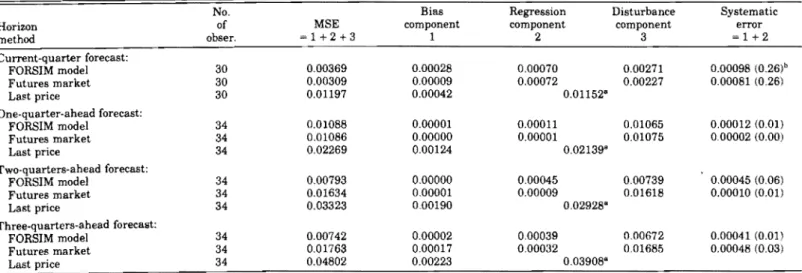
The data in Table 2 show the components of the mean square error for lumber price forecasts, by method and forecast horizon. In all cases, the bias component is very small relative to the total error, especially for the FORSIM model and the futures market. The systematic error of the FORSIM model for forecasts made one to three quarters ahead varies between 1 and 6 percent of the total error. This suggests that there is little room for improving those forecasts. On the other hand, the sys tematic error represents 27 percent of the total error made by FORSIM for the current quarter forecasts. This is about the same for the futures market and may be due simply to the difficulty of measuring the current-period forecast errors, as noted earlier.
TABLE 1. - Comparison of forecast errors for lumber prices predicted
three methods and for four horizons (1974·1 to 1980-1). Method
Forecast
horizon FORSIM Futures market Last price
Current quarter (N 30)
RMSE 0.06 0.06 0.11
---. bij
FORSIM 0.04 -0.53***
Futures market -0.61***
One quarter ahead (N 34)
RMSE 0.10 0.10 0.15
--- bij
FORSIM 0.00 -0.25**
Futures market -0.24**
Two quarters ahead (N 34)
RMSE 0.09 0.13 0.18
.---•••••--- bij
FORSIM -0.24** -0.45***
Futures market -0.20**
Three quarters ahead (N = 34)
RMSE 0.09 0.13 0.22
---••. -•••--•••---.-- b'i ._.._.._---_..__.._..._..
FORSIM -0.27*** -0.53***
Futures market -0.27***
Notes: RMSE is the root mean square error, bij is the test statistic
differences between errors by methods i (row) and) (column). *, **,
and *** indicate significant differences at the 0.90, 0.95, and 0.99 confidence level, respectively. N is the number of observations.
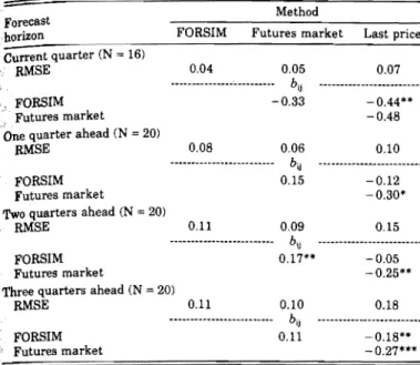
Similar results for plywood prices are reported in Tables 3 and 4. Table 3 shows that the FORSIM model and the futures market provided forecasts that did not differ significantly, except for forecasts made two quar ters ahead, in which case the futures market did sig nificantly better than the FORSIM model, reducing the average forecast error by 2 percent. For one-quarter and two-quarters-ahead forecasts, the FORSIM model was not significantly more accurate than the last ply wood price.
The results on the components of the mean square error for plywood price forecasts (Table 4) show that, as for lumber, the systematic error of the FORSIM model is a small component of the total error. For the FORSIM model, the systematic error varies between 0.3 and 5 percent of the total error for forecasts made one to three quarters ahead. The systematic error is higher for the current quarter (10% of total error) but this may again be due to difficulties of definition. Therefore, as for lumber, there seems to be only limited room for im provement in the FORSIM forecasting methodology. Systematic errors are generally larger for the futures market. This indicates some inefficiency in the plywood futures market, perhaps due to insufficient trading activity.
The results of the analysis of turning point errors are summarized in Table 5. This analysis was done only for forecasts made one quarter ahead. The results are in agreement with those of the mean-square error analy sis. For lumber, the FORSIM model made less turning" point errors, of both kinds, than the futures market. The reverse was true for plywood where the futures market was better at forecasting turning points than the
FORSIM model. During the period 1974-1 to 1980-1,
setting the price next quarter equal to last quarter's would have been a good way of predicting turning points.
Summary and conclusions
The object ofthis paper was to evaluate the absolute and comparative accuracy of three methods of
fore-TABLE 2. - Comparison of MSE and its components for lumber price by horizon and method offorecast (1974-1 to 1980-1).
No. Bias Regression Disturbance Systematic
Horiron of MSE component component component error
obser. =1+2+3 1 2 3 =1+2 Current-quarter forecast: FORSIM model 30 0.00369 0.00028 0.00070 0.00271 0.00098 (0.26)b Futures market 30 0.00309 0.00009 0.00072 0.00227 0.00081 (0.26) Last price 30 0.01197 0.00042 0.01152" One-quarter·ahead forecast: FORSIM model 34 0,01088 0.00001 0.00011 0.G1065 0.00012 (0.01) Futures market 34 0.G1086 0.00000 0.00001 0.01075 0.00002 (0.00) Last price 34 0.02269 0.00124 0.02139" Two-quarters-ahead forecast:
FORSIM model 34 0.00793 0.00000 0.00045 0.00739 0.00045 (O.06)
Futures market 34 0.01634 0.00001 0.00009 0.01618 0.00010 (0.01) Last price 34 0.03323 0.00190 0.02928" Three-quarters-ahead forecast: FORSIM model 34 0.00742 0.00002 000039 0.00672 0.00041 (0.01) Futures market 34 0.01763 0.00017 0.00032 0.01685 0.00048 (0.03) Last price 34 0.04802 0.00223 0.03908"
"The Sf; of the lagged price being zero, the MSE couldn't be decomposed into these three components. bFraction of MSE that is systematic. Components may not add up to MSE due to round off errors.
JULY/AUGUST 1984
, TABLE 3,
-, three methods and for four horizons (1974·1 to 1981·I).
FORSIM Futures market
One quarter ahead (N = 20)
Comparison offorecast errors for plywood prices predicted casting the price of lumber and plywood. The first
method, used by Data Resources Inc., is based on a large econometric model (FORSIM) supplemented by judg
FORSIM Futures market Last price ment. The second is based on prices of contracts traded
on the futures market. The third method is a naive
0.04 0.05 0.07 forecast equating the price in the future to the last
.•.•...•••• -... bij
known cash price.
-0.33 -0.44**
-0.48 Due to the data available, quarterly forecasts were
compared, with horizons ranging from the current quar
RMSE 0.08 0.06 0.10
••••••••...•••••••••••... by ter to three quarters ahead. For lumber the FORSIM
:~,
FORSIM 0.15 -0.12 model, during the period 1974-1 to 1980-1, produced
Futures market -0,30· forecasts that were significantly more accurate than the
~{ Two quarters ahead (N 20) futures markets when forecasts were made two to three
RMSE 0,11 0,09 0,15
...••••••••.•••••.••••••• bij ...••••••••....•••••••••• quarters ahead. But there was no significant difference
FORSIM 0.17*· -0.05 for current-quarter forecasts and those made one quar
Futures market -0,25** ter ahead. The root mean square errors of the FORSIM
Three quarters ahead (N = 20) forecasts ranged between 6 and 10 percent. Those of the
RMSE 0.11 0.10 0.18
••••.••.•••••••••.•••.••. bij ...•..••••.•••••••..••• futures market ranged between 6 and 13 percent. Both
FORSIM 0.11 -0,18*· futures market and FORSIM were significantly more
;,,' Futures market -0.27*** accurate than the naive forecasts.
For plywood, the futures market was significantly more accurate than the FORSIM model for forecasts
.,:"--". made two quarters ahead. But there was no significant
difference between these two methods for the other forecast horizons. Forecast errors ranged between 4 and 11 percent for both methods, increasing with the length of the forecast. For one-quarter- and two-quarters
-~-;:~ !t%~~,. ~ ~~~"'" ~~~~": ~~t'~-,~f . :::.i,=====T=A=B=L=E=4,==C=o=m~p=a=ri=so=n=o~f==M=S=E=a=nd=it=s=d=l?c=o=m::p=os=it=io=n=,,,=o=rp,=l::y=w=ood==,p,=r=ic=e=b::y=h=o=riz=o=n:::::a=n=d=m=et=ho=d==of=,,=or=e=cas=t=(1=9=74=.=I=to=19=8=1=.I=),=====
~\, No, Bias Regression Disturbance Systematic
,:,,'i'Horizon of MSE component component component error
};~!;",;method obser. 1+2+3 1 2 3 =1+2
:pVii
.y:~:' Current·quarter forecast:
&:,.r,\:' FORSIM model 16 0.00155 0.00010 0,00005 0,00140 0.00015 (0.10)b
~"';/';Futures market 16 0.00302 0.00033 0,00162 0.00107 0.00195 (0.65)
c'¥t Last price 16 0.00517 0,00020 0.00497"
~?\-"
11;~,< ,One-quarter· ahead forecast:
!:~;, FORSIM model 20 0.00608 0.00001 0,00002 0.00606 0.00002 (0,00)
~;~» Futures market 20 0,00407 0,00000 0.00002 0.00404 0,00002 (0.00)
~f~l Last price 20 0.01045 0.00174 0.00850"
~i::}Two.quarters.ahead forecast:
~:,'i FORSIM model 20 0.01260 0.00032 0.00036 0.01220 0.00068 (0.05)
~~:jFuture~ market 20 0.00747 0.00078 0,00024 0,00673 0,00102 (0.14)
~0'. ,if ,Last pnce 20 0,02139 0,00648 0.01473"
~~\' Three·quarters·ahead forecast:
.~;, ," FORSIM model 20 0,01313 0.00004 0,00007 0.01306 0.00012 (0,01)
~;,./ Futures market 20 0.01018 0.00128 0.00039 0.00871 0,00167 (0.16)
~:. Last price 20 0.03417 0.01022 0.02353"
t;'
"The Sn of the naive model at current period forecast is zero; the MSE couldn't be decomposed into these three components.;'., :bFraction of MSE that is systematic. Components may not add up to MSE due to round off errors,
TABLE 5. - Frequencies of turning points of lumber and plywood prices, predicted over one quarter by three methods.
Errors
1st 2nd
Method Predicted kind kind
•••.•••••.•..•••...•.••••••...•..•..•...•••... (Lumber) ... FORSIM 12 14 10 2 4 0.17 0.29 FutUres market 10 14 7 3 7 0,30 0,50 Last price 23 14 14 9 o 0.39 0,00 .••. _ •.•••...•...-... (Plywood) •••••••••...•.•••...••.•••...•...•...•.•....•.••..•.•. FORSIM 12 10 7 5 3 0.42 0,30 Futures market 12 10 8 3 2 0,27 0,20 Last 17 10 9 8 1 0.47 0.10
FOREST PRODUCTS JOURNAL Vol. 34, No. 7/8
ahead forecasts, FORSIM did not improve upon the
naive model. The same was true for the futu~es market
for current-quarter forecasts. I
Analysis of the mean square errors showed that FORSIM and the futures market do give unbiased fore casts. In addition, most of the error of FORSIM price forecasts appeared to be of a random nature, leaving limited room for improvements in methodology. Turn ing points of lumber and plywood price were predicted best by the lagged cash price.
In comparing the various methods one must keep in mind that the FORSIM model forecasts many variables besides prices, including production, demand, inven
tories, etc. It is possible to conceive a model that would
provide better price forecasts only. The time-series methodology seems attractive in that respect (1,12), but a time-series model would not provide as much infor mation. Still, as econometric models become more wide spread, it will be useful to continue monitoring their forecasting performance, and to compare econometric models with alternative methods, including the futures market. This study stopped in 1980-1, due to the change in the definition of the lumber contract from hem-fir to spruce-pine-fir. The forecasting potential of the lumber futures market under the current contract should be investigated as soon as enough data are available. Un fortunately, the futures market for plywood may close soon due to insufficient trading activity.
Literature cited
1. BUONGIORNo,J.,andJ.BALSIGER.1977. Quantitative analysis and forecasting of monthly prices oflumber and flooring products. Ag. Systems 2:165-18l.
2. DANTHINE, J. 1978. Information, futures prices, and stabilizing speculation. J. Econ. Theory 17:79-98.
3. DATA RESOURCES, INC. 1974-1981. FORSIM review. Data Re sources, Inc., Lexington, Mass.
4. GARDNER, B.L. 1976. Futures prices in supply analysis. Am. J. Agr. Econ. 58:81-84.
5. GRANGER, C.W.J. 1980. Forecasting in Business and Economics. Academic Press, Inc., New York, 226 pp.
6. GREEN, J. 1981. Value of information with sequential futures market. Econometrica 49:335-358.
7. JUST, R.E., and G.C. RAUSSER. 1981. Commodity price forecasting with large-scale econometric models and the futures markets. Am. J. Agr. Econ. 63(2):197-208.
8. KOFI, T.A. 1973. A framework for comparing the efficiency of futures markets. Am. J. Agr. Econ. 55:584-594.
9. MADDALA, G.S. 1977. Econometrics. McGraw-Hill, New York. 10. MARTIN, L., and P. GARCIA. 1981. The price.forecasting perform
ance of futures market for live cattle and hogs: a disaggregated analysis. Am. J. Agr. Econ. 63(2):209·215.
11. NETER, J., and W. WASSERMAN. 1974. Applied linear statistical models-regression, analysis of variance and experimental designs. Richard D. Irwin, Inc.
12. OUVEIRA, R.A., J. BUONGIORNO, and A.M. KMIOTEK. 1977. Time· series forecasting models oflumber, cash, futures and basis prices. Forest Sci. 23(2):268·280.
13. RANDOM LENGTHS. 1973-1981. Random Lengths Annual Yearbook, Eugene, Oreg.
14. THEIL, H. 1970. Economic Forecasts and Policy. North·Holland Publishing Company, Amsterdam.
15. TOMEK, W .G., and R. W. GRAY. 1970. Temporal relationship among prices on commodity futures markets: their allocative and stabiliz ing roles. Am. J. Agr. Econ. 52:372-380.
16. VELTKAMP,J.J., R. YOUNG, andR. BERG. 1983. The Data Resources Inc., approach to modeling demand in the softwood lumber and
plywood and pulp and paper industries. In Forest Sector Models. R.
Seppala, C. Row, A. Morgan, Eds. AB Academic Press, Berkham· sted, England.
17. WHITEMAN, I.R.1966. Improved forecasting through feedback. J. of
Marketing 30(2):45.
Appendix
The decomposition of the MSE is done in the fol
lowing manner. Let r denote the correlation between
relative forecast price ft.,; and relative actual price at,;
n
2:
(ft.
i - 1) (at,;r= t 1 '
(
tl11,1~
<"t' -
Ii f)2~
(at.i - ili)2) 112n
lin
2:
(ft.
i ~) (lZt.i - aj)/SF Sa·I 1
t = 1 '
Thus n
MSE = lin
2:
(ft.
i - at,j)2t= 1 '
(r; -
a)2 + (Sfi - rSai)2 + (1 - r2)Sai2 (14, p. 38)=
(~-
aj)2 +Sf,
(1 - r Sa/Sfi)2 + (S;irS;;)
=
cr;
ai)2 + S~ (1 ~)2 + (S;j ~2&i2)n
«(; -
aj)2+
Sn~l-
~)2 + lin2:
(€t i - €j)2t 1 '
where ~ and aj are the sample means ofthe forecast and
actual relative prices for the ith forecast horizon;
S¥.
represents the sample variance of ft,j; ~ and €t,i are the estimated coefficient and the residual obtained by re gressing the actual relative price aj".j on the forecastrelative price
ft.,i'
The first term in the MSE equation,called the bias component, indicates the extent to which
the magni tude of the MSE is the consequence of a tendency to estimate too great or too small a change of the forecast price. The second and third terms are called the regression and disturbance components of the MSE, respectively, for the following reason (9, p. 345). The actual relative prices al.i> ... an.j can be viewed as con
sisting each of a random (€t,i) and nonrandom (0: + ~ ft,j) part, Le.,
at +1 ·::= 0: + Cl.l't·+ P/i.l €t' ,I 0,1,2,3
t ::= 1, ... , n .
assuming that the random part has zero mean. Ifthe
prediction is perfect on the nonrandom part, then, 0: 0,
~
=
1 and at+i = ft.,i + €t,i' In that case, both the bias and regression components are equal to zero, and the MSEjisequal to the variance of the residual (€t,J This residual,
or random part is unpredictable, therefore, the best that forecasting methods can do is to minimize the bias and the regression components, Le., the "systematic" errors.
JULY/AUGUST 1984 18