Adomian's decomposition method for eigenvalue problems

Adomian’s decomposition method for eigenvalue problems

Yee-Mou Kao1and T. F. Jiang2

1

Institute of Applied Mathematics, National Chiao-Tung University, Hsinchu 30010, Taiwan

2

Institute of Physics, National Chiao-Tung University, Hsinchu 30010, Taiwan

共Received 10 September 2004; published 8 March 2005兲

We extend the Adomian’s decomposition method to work for the general eigenvalue problems, in addition to the existing applications of the method to boundary and initial value problems with nonlinearity. We develop the Hamiltonian inverse iteration method which will provide the ground state eigenvalue and the explicit form eigenfunction within a few iterations. The method for finding the excited states is also proposed. We present a space partition method for the case that the usual way of series expansion failed to converge.

DOI: 10.1103/PhysRevE.71.036702 PACS number共s兲: 02.70.Wz, 03.65.Ge

I. INTRODUCTION

Adomian’s method solves nonlinear differential equations with decompositions. Neither linearization nor perturbation is applied to the nonlinear part. The method has been widely applied to various domains in science and engineering, but is less popular in physics. Actually, in Chap. 14 of Adomian’s comprehensive book 关1兴, he treated many physical topics, namely, the Navier-Stokes equations, onset of turbu-lence, Burger’s equation, nonlinear transport, advection-diffusion equation, Korteweg–de Vries equation, nonlinear Schrödinger equation共NLSE兲, and classical N-body dynam-ics, etc. It shows that Adomian’s decomposition method

共ADM兲 is extremely versatile in nonlinear physical

prob-lems. For some other examples, Adomian and co-workers also formulated the solutions for Thomas-Fermi equation关2兴 and the Ginzburg-Landau equation 关3兴. Wazwaz employed ADM to give the soliton and periodic solutions of the Bouss-inesq equation关4兴. Abbaoui et al. discussed the convergence of the ADM关5兴. Guellal et al. gave the ADM explicit solu-tion of the Lorenz system关6兴.

The ADM is generally applicable to nonlinear differential equations for either initial value problems or boundary prob-lems. The basic theory is clearly described in Adomian’s book 关1兴. On the other hand, we are not able to find out systematic treatment for the eigenvalue problems by ADM. Since the eigenvalue problem is fundamentally important for the structure of a system, the pursuit of ADM for the eigen-value problem is a worthwhile work. It is, nevertheless, not straightforward. Also, the ADM gives an explicit form of solutions that the numerical grids method cannot do. Thus the ADM treatment of the eigenvalue problem is valuable to computational physics. In this paper, we develop the method for solving the eigenvalue problems by ADM. We will briefly describe the ADM first, and then present our method for the eigenvalue problem. Some paradigmatic examples of both linear and nonlinear eigenvalue equations are given.

The paper is organized as follows. In Sec. II, we introduce the Hamiltomian inverse iteration scheme for the ADM of eigenvalue problems. In Sec. III, we apply the method to the problem of a particle in a box. In Sec. IV, the method is applied to the simple harmonic oscillator. Section V is a

treatment of the anharmonic oscillator, and in Sec. VI, we try to solve the nonlinear Gross-Pitaevskii equation that de-scribes the Bose-Einstein condensate by the new scheme. We find that the straightforward way of ADM failed to converge. We introduce in Sec. VII the space partition method to over-come the trouble of divergence encountered in the previous section. Section VII is devoted to concluding remarks.

II. HAMILTONIAN INVERSE ITERATION Consider the general eigenvalue problem

Hu共x兲 = ␭u共x兲, 共1兲

where

H = L + V„u共x兲…. 共2兲

L is usually a differential operator such as − 1

Ⲑ

2共d2/ dx2兲 and V(u共x兲) is the potential function, either dependent or independent of u共x兲. The former case is a linear problem while the latter case is nonlinear and is called a nonlinear Schrödinger equation. We describe the difficulty in the ADM for eigenvalue problems first. Adomian wrote the solution as the sum of decompositions

u共x;⑀兲 =

兺

n=0 ⬁

⑀n_u

n共x兲. 共3兲

Expand the potential V(u共x;⑀兲),

V„u共x;⑀兲… =

兺

n=0 ⬁

⑀n_A

n; 共4兲

here we introduce the parameter⑀to collect the coefficients of same order in both sides to find out the decompositions A_n for a general V. The introduced ⑀ is set equal to 1 at last. Some examples of Ancan be found in Ref. 关1兴 and will not be repeated here. Let L−1 _{be the inverse operator of L.} Op-erating the L−1 _{to Eq.共1兲, we have}

L−1Lu =␭L−1u − L−1V. 共5兲

The solution of decomposition orders are obtained system-atically关1兴. That is,

u₀共x兲 = c₀+ c₁x, u_k+1共x兲 = ␭L−1_u

k− L−1Ak, 共6兲 where c0 and c1 are the integration constants generated by the double integration of L−1_{. They can be determined either} by symmetric property or by the boundary condition. For the eigenvalue problems, the value of␭ is unknown, the scheme does not work mainly due to the accumulation of unknown␭ into higher orders during the iterations. Thus the ADM to the eigenvalue problems is not straightforward.

The inverse iteration is a powerful procedure to compute the eigenfunctions and eigenvalues of a linear system 关7兴. The basic idea of our Hamiltonian inverse iteration follows that for linear system. Consider an initial trial solution⌿₀of Eq.共1兲, ⌿0 in principle will be a linear combination of the eigenfunctions兵␾n其:

⌿0=

兺

n=0 ⬁

cn␾n. 共7兲

Repeatedly applying the inverse Hamiltonian operator to⌿0 leads to 关H−1_兴k_⌿ 0=

兺

n=0 ⬁ c_n ␾n 共␭n兲k . 共8兲

Without loss of generality, we assume the eigenspectrum is

兵0⬍␭0⬍␭1⬍␭2⬍¯其. For sufficiently large value of k, the remaining of iterations will be dominated by the ground state eigenfunction only.

Symbolically, given an initial ⌿0, and denoting the ap-proximate eigenvalue of the kth iteration by␭k, we have, for the next iteration⌿k+1,

H−1⌿k= 1

␭k

⌿k+1, 共9兲

where the⌿

⬘

s are renormalized at the end of each iteration.

Convergence of the inverse iteration toward an eigenstate can be estimated by the Rayleigh Quotients共RQ兲, which are given by

␭k=

冕

⌿kH⌿k+1dx. 共10兲

The eigenvalue of the ground state is the stationary point of

␭k

⬘

s,

lim k→⬁⌿k

=␾₀, and H␾₀=␭₀u_0. 共11兲

We call this procedure the Hamiltonian inverse iterations

共HII兲. If we project out the obtained ground state␾0from the initial trial function⌿0, the HII will lead to the next higher eigenstate. The excited states can thus be found by HII, too. Next, we will estimate the number of iteration steps to reach a given accuracy in the eigenvalue. Consider we are solving the nth eigenstate for a system. After k times HII iteration procedures, we may denote the result as a factor of

共1−⑀兲 in the component of ␾n and a factor of⑀ in the next higher state␾_n+1. The components in other higher states are

negligible through the HII scheme. So the expectation value of the eigenvalue is

具␭n典k=共1 −⑀兲␭n+⑀␭n+1, 共12兲 hence the error is

␦k=具␭n典k−␭n=⑀共␭n+1−␭n兲 . 共13兲 Iterate one more time, the component in ␾n becomes

C_k+1共1−⑀兲/␭_n, and the component of ␾_n+1 is C_k+1⑀/␭_n+1, where C_k+1 is the normalization constant. Assume ⑀is very small, then Ck+1= 1 共1 −⑀兲/␭n+⑀/␭n+1 ⯝ ␭n

冋

1 +⑀

冉

1 − ␭n ␭n+1

冊

册

. 共14兲

Thus the expectation of the eigenvalue will be

具␭n典k+1⯝

冉

1 −⑀ ␭n ␭n+1

冊

␭n+ ␭n ␭n+1 ⑀␭n+1. 共15兲 The error now will be

␦k+1=具␭n典k+1−␭n=⑀ ␭n ␭n+1 共␭n+1−␭n兲 =

冉

␭n ␭n+1

冊

␦k. 共16兲

It means that when we iterate one more time, the error will be smaller by a factor of␭_n/␭_n+1. To reach the Nth decimal place accuracy in eigenvalue, the number of iterations can be estimated to be N / log共␭n+1/␭n兲.

III. EXAMPLE OF THE PARTICLE IN A BOX We start to explore the method with the simple problem of a particle in a box. Its eigenstates are analytically known. The potential V共x兲 is V共x兲 =

冦

⬁, x ⬍ −␲ 2, 0, −␲ 2 ⬍ x ⬍ ␲ 2, ⬁, ␲ 2 ⬍ x. 共17兲

The Hamiltonian operator for the particle inside the box is

H = −1

2

d2

dx2, 共18兲

and the boundary conditions at the box ends are

␺

冉

x = ±␲

2

冊

= 0. 共19兲

Using the notation Lxx= d2/ dx2 and H−1= −2Lxx −1

, by the HII method, the relationship between consecutive iterations is

⌿1= H−1⌿0= − 2Lxx −1_⌿

0. 共20兲

⌿0共x兲 =

兺

n=0

a0,nxn, and ⌿1共x兲 =

兺

n=0

a1,nxn, 共21兲

then the HII leads to the following coefficient relations:

a1,0= C1 共an unknown integration constant兲,

a1,1= C2 共an unknown integration constant兲,

¯ a_1,k= − 2

k共k − 1兲a0,k−2. 共22兲

We can assign the unknown constants by the parity of the wave function in this case. For the ground state, C₂= 0. we arbitrarily use the starting trial function ⌿0共x兲=1−共2x/␲兲2. The⌿1derived from Eq.共15兲 is used as the new trial func-tion. We iterate to k = 7, the eigenvalue obtained is accurate to 15 decimal places. And the obtained coefficients give us an explicit form of the ground state eigenfunction. For the first excited state, symmetry requires C₁= 0. We use ⌿₀共x兲 = x关1−共2x/␲兲2兴, the iterations to k=16 provides the eigen-value accurate to 10 decimal places, and iterations to k = 24 leads to 15 decimal places accuracy.

IV. EXAMPLE OF THE SIMPLE HARMONIC OSCILLATOR

The next example is the classic case of the simple har-monic oscillator. Again, the eigenstates are analytically known. The potential V共x兲 now is

V共x兲 =1

2x

2_{, 共23兲}

with the boundary condition

␺共x → ± ⬁兲 → 0. 共24兲

By the HII method, the relation of iteration is

⌿0= − 1 2Lxx⌿1+ 1 2x 2_⌿ 1. 共25兲

Assume the decomposition forms

⌿i共x兲 =

兺

n=0

ai,nxn, with i = 0,1 共26兲 and the coefficient relations from HII are

a0,0= − 2⫻ 1 2 a1,2, a0,1= − 3⫻ 2 2 a1,3, a0,2= − 4⫻ 3 2 a1,4+ 1 2a1,0, ¯ a_0,k= −共k + 2兲共k + 1兲 2 a1,k+2+ 1 2a1,k−2, k⬎ 2. 共27兲 In terms of the power of x,

x0: a1,0= C1 共an unknown integration constant兲,

x1: a1,1= C2 共an unknown integration constant兲,

x2: a1,2= − a0,0,

¯ xk: a1,k=

1

k共k − 1兲共a1,k−4− 2a0,k−2兲. 共28兲

To find the integration constants C₁ and C₂, we regroup the wave function⌿1into three parts

⌿1=⌿␣+ C1⌿␤+ C2⌿␥, 共29兲 where ⌿␣=

兺

n=0 a_␣,nxn, ⌿_␤=

兺

n=0 a_␤,nxn, ⌿_␥=

兺

n=0 a_␥,nxn. 共30兲

Then we have the following relationships for the three series:

x0_{: a} ␣,0= 0, x1: a_␣,1= 0, x2: a_␣,2= − 2 2⫻ 1a0,0, x3_{: a} ␣,3= − 2 3⫻ 2a0,1, ¯ xk: a_␣,k= 1 k共k − 1兲共a␣,k−4− 2a0,k−2兲 ; 共31兲 and x0: a_␤,0= 1, x1: a_␤,1= 0, x2: a_␤,2= 0, x3: a_␤,3= 0, ¯ xk:a_␤,k= 1 k共k − 1兲a␤,k−4; 共32兲 and

x0_{: a} ␥,0= 0, x1: a_␥,1= 1, x2: a_␥,2= 0, x3: a_␥,3= 0, ¯ xk: a_␥,k= 1 k共k + 1兲a␥,k−4. 共33兲

We choose the boundary ⌿1共L兲=0 at L=6.0. For the ground state, we set⌿0= e−x

2

and expand it to the power of 200 in x for iteration, at k = 12 the eigenvalue is accurate to 10 decimal places; and at k = 15 the accuracy is up to 15 decimal places. For the first excited state, we choose ⌿0 = xe−x2, at k = 15 the eigenvalue is accurate to 10 decimal places, and at k = 33 the accuracy is up to 13 decimal places.

V. EXAMPLE OF THE ANHARMONIC OSCILLATOR We consider in the following the anharmonic oscillator that was recently treated by the imaginary time propagation method关8兴. It provides the calibrations of our method. The potential form is

V共x兲 =1

2x 2₊

v4x4+v6x6, 共34兲 and the boundary condition is the same as the simple har-monic oscillator. By the HII method, the relationship be-tween iterations is ⌿0= − 1 2Lxx⌿1+

冉

1 2x 2₊ v4x4+v6x6

冊

⌿1; 共35兲 as in the previous power series expansion, the coefficient relations are a0,0= − a1,2, a0,1= − 3⫻ 2 2 a1,3, a0,2= − 4⫻ 3 2 a1,4+ 1 2a1,0, a0,3= − 5⫻ 4 2 a1,5+ 1 2a1,1, a0,4= − 6⫻ 5 2 a1,6+ 1 2a1,2+v4a1,0, a0,5= − 7⫻ 6 2 a1,7+ 1 2a1,3+v4a1,1, ¯ a0,k= − 共k + 2兲共k + 1兲 2 a1,k+2+ 1 2a1,k−2+v4a1,k−4 +v6a1,k−6, when k艌 6.

In terms of the power of x,

x0: a1,0= C1 共an unknown integration constant兲,

x1: a1,1= C2 共an unknown integration constant兲,

x2_{: a} 1,2= − 2 2⫻ 12a0,0, x3: a1,3= − 2 3⫻ 2a0,1, x4: a1,4= 1 4⫻ 3共a1,0− 2a0,2兲, x5: a1,5= 1 5⫻ 4共a1,1− 2a0,3兲, ¯ xk: a1,k= 1 k共k − 1兲共a1,k−4+v4a1,k−6+v6a1,k−8− 2a0,k−2兲. 共36兲

We again regroup the power series into⌿_␣,⌿_␤, and⌿_␥. The integration constants C1 and C2 can be found by Eq. 共29兲. For ground state withv4= 0.02, andv6= 0.01关8兴, we choose

⌿0= e−x

2_/2

and expand to the power of x up to 200. Iterations to k = 12 and set cutoff at L = 4.5, the eigenvalue is accurate to nine decimal places. For the first excited state, take ⌿0 = xe−x2/2and expand to the power of x up to 200. Iterations to

k = 20 gives the eigenvalue accurate up to eight decimal

places.

VI. EXAMPLE OF NLSE, THE GROSS-PITAEVSKII EQUATION

In the recent Bose-Einstein condensation experiments of dilute alkali atomic gases 关9兴, the condensate is well de-scribed by the mean-field approximation, that is, the Gross-Pitaevskii equation共GPE兲. Furthermore, if the trap potential is cigar shaped, the GPE is effectively one dimensional关10兴. Following the pseudospectral method 关11兴, we have devel-oped an efficient and accurate numerical scheme for solving the GPE. Our pseudospectral method has been calibrated with published calculations关12兴 and provides a way to jus-tify our new ADM of eigenvalue problems.

冉

−1 2

d2

dx2+ V共x兲 + g兩⌿兩

2

冊

_{⌿ =␮⌿, 共37兲} with the order parameter normalized to the number of con-densed atoms

冕

−⬁

⬁

兩⌿兩2_{dx = N. 共38兲}

By the HII, the iteration relationships are

⌿0=

冉

− 1 2 d2 dx2+ V共x兲 + g兩⌿0兩 2

冊

_⌿ 1. 共39兲 We expand 兩⌿₀兩2_=␳=兺

i␳ixi, and the nonlinearity into de-compositions

g␳⌿1=

兺

i

Aixi. 共40兲

The coefficient relationships are

a0,0= A0− 2⫻ 1 2 a1,2, a0,1= A1− 3⫻ 2 2 a1,3, ¯ a0,k= Ak− 共k + 2兲共k + 1兲 2 a1,k+2+ 1 2a1,k−2. 共41兲 In terms of the power of x,

x0: a1,0= C1 共an unknown integration constant兲,

x1: a1,1= C2 共an unknown integration constant兲,

x2: a1,2= A0− a0,0, x3: a1,3= 2 3⫻ 2共A1− a0,1兲, ¯ xk: a1,k= 2 k共k − 1兲

冉

Ak−2− a0,k−2+ 1 2a1,k−4

冊

. 共42兲 We again regroup it into⌿_␣,⌿_␤, and⌿_␥to find the integra-tion constants C1 and C2, by Eq. 共29兲. The three nonlinear terms are expanded as

A_␣= g␳⌿_␣=

兺

i=0 A_␣,ixi_{, 共43兲} and A_␤= g␳⌿_␤=

兺

i=0 A_␤,ixi, 共44兲 and A_␥= g␳⌿_␥=

兺

i=0 A_␥,ixi. 共45兲

Then the relationships become

x0: a_␣,0= 0, x1: a_␣,1= 0, x2: a_␣,2= A_␣,0− a_␣,0, x3: a_␣,3= 2 3⫻ 2共A␣,1− a0,1兲, ¯ xk: a_␣,k= 2 k共k − 1兲

冉

A␣,k−2− a0,k−2+ 1 2a␣,k−4

冊

; 共46兲 and x0: a_␤,0= 1, x1: a_␤,1= 0, x2: a_␤,2= A_␤,0, x3: a_␤,3= 2 3⫻ 2共A␤,1兲, ¯ xk: a_␤,k= 1 k共k − 1兲共2A␤,k−2+ a␤,k−4兲; 共47兲 and x0: a_␥,0= 0, x1: a_␥,1= 1, x2: a_␥,2= A_␥,0, x3: a_␥,3= 2 3⫻ 2共A␥,1兲, ¯ xk: a_␥,k= 1 k共k − 1兲共2A␥,k−2+ a␥,k−4兲. 共48兲

For the trap with parameters g = 0.017 84 and N = 100, by using the trial function e−x2/2, and cutoff at L = 2.38. We ob-tain ␭=1.1684 for iterations up to k=16. However, if we extend the cutoff L to larger value, the direct use of power series expansion in ADM does not converge, and no solution will be found. So the eigenvalue␭=1.1684 is not the correct ground state. This happens if the cutoff lies beyond the

ra-dius of convergence for the power series expansion. To over-come the trouble, we develop the space partition method in the next section.

VII. SPACE PARTITION METHOD FOR ADM EIGENVALUE PROBLEMS

To justify the convergence of series expansion, we divide the space 关0,L兴 into p partitions 关Xm−1, Xm兴,m = 1 , 2 , 3 , . . . , p. And the iteration function⌿kin the mth par-tition is denoted as⌿k,m共x兲 with x苸关Xm−1, Xm兴. The global solution is given by ⌿k共x兲 =

兺

m=1 p ⌿k,m共x兲␹m共x兲, x 苸 关0,L兴, 共49兲 where ␹m共x兲 =

再

1, x僆 关Xm−1,Xm兴, 0, x⫽ 关Xm−1,Xm兴, 共50兲 and 关0,L兴 = 艛 m=1 p 关Xm−1,Xm兴. 共51兲

In mth partition, note that the potential V共x兲 become

V共Xm−1+ x兲.

We choose L = 6 , p = 6, and Xm= m, the connection condi-tion at x = Xmis M_m共1兲C_m= M_m+1共0兲C_m+1, 1艋 m 艋 p − 1, 共52兲 Mp共1兲Cp= B, 共53兲 where Mm共x兲 =

冤

1 0 0 ⌿␣,m共x兲 ⌿␤,m共x兲 ⌿␥,m共x兲 ⌿_␣,m

⬘

共x兲 ⌿_␤,m

⬘

共x兲 ⌿_␥,m

⬘

共x兲

冥

, 共54兲

where Mm共0兲=I and

Cm=

冤

1 C_m,1 Cm,2

冥

, B =

冤

1 0 ⌿k

⬘

共L兲

冥

. 共55兲 with unknown⌿_k,m

⬘

共L兲.

For the even parity ground state, C_1,1= 0. we have 2p − 1 unknown constants. The order parameter and its first deriva-tive must be continuous at the junctions of partitions, and

⌿k共L兲=0, so the number of constraints is also equal to 2p − 1. To find the M_m共1兲, B = Mp共1兲Cp= Mp共1兲Mp−1共1兲Cp−1 = Mp共1兲Mp−1共1兲Mp−2共1兲¯ M1共1兲C1 = MC1, 共56兲 where M = Mp共1兲Mp−1共1兲Mp−2共1兲¯M1共1兲. We determine

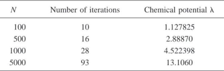
C1,2and ⌿1,1by the Eq. 共56兲, and the next neighbor order parameter by the Eq.共52兲. The total ⌿1can then be obtained. With the space partition method, we overcome the prob-lem of convergence. The results of some calculations are shown in Table I.

VIII. CONCLUSION

Adomian’s decomposition method together with the Hamiltonian inverse iteration technique provide a simple and powerful tool for the eigenvalue problems. Unlike other nu-merical grids methods, the ADM technique gives explicit form of solution. Moreover, although we showed only the decomposition solutions for differential equations, the method is applicable to algebraic equations, too.

The inverse iteration for finding the eigenfunctions and eigenvalues is well known in matrix theory, but applications to differential equations are not common. The difficulty lies particularly in writing down the inverse of the Hamiltonian. But with the ADM, we have found a way to do it. Combining the Hamiltonian inverse iteration and Adomian’s decomposi-tion method, we have developed an efficient algorithm to solve the general eigenvalue problem. We show that the new method works well for both the linear and nonlinear prob-lems. Even for the nonlinear case, only a few iterations are required to achieve high accurate results, while using our pseudospectral method for Gross-Pitaevskii takes far more steps of iterations.

A drawback of the ADM is the constraint of the boundary condition, especially when the size of boundary is larger than the radius of convergence of the expansion series of the wave function. We develop the partition of the space method and overcome this trouble.

ACKNOWLEDGMENT

The research of T.F.J. was supported by the National Sci-ence Council of Taiwan under Contract No. NSC92-2112-M009-004.

TABLE I. The eigenvalues of the Gross-Pitaevskii equation cal-culated by the space partition method for N bosons.

N Number of iterations Chemical potential␭

100 10 1.127825

500 16 2.88870

1000 28 4.522398

关1兴 G. Adomian, Solving Frontier Problems of Physics: The

De-composition Method共Kluwer, Dordrecht, 1994兲.

关2兴 G. Adomian, Appl. Math. Lett. 11 共3兲, 131 共1998兲.

关3兴 G. Adomian and R. E. Meyers, Comput. Math. Appl. 29 共3兲, 3 共1995兲.

关4兴 A. M. Wazwaz, Chaos, Solitons Fractals 12, 1549 共2001兲. 关5兴 K. Abbaoui and Y. Cherruault, Comput. Math. Appl. 28 共5兲,

193共1994兲.

关6兴 S. Guellal, P. Grimalt and Y. Cherruault, Comput. Math. Appl. 33共3兲, 25 共1997兲.

关7兴 I. Ipsen, SIAM Rev. 39, 254 共1997兲.

关8兴 A. K. Roy, N. Gupta, and B. M. Deb, Phys. Rev. A 65, 012109 共2001兲.

关9兴 M. H. Anderson et al., Science 269, 198 共1995兲; C. C. Bradley

et al., Phys. Rev. Lett. 75, 1687共1995兲; K. B. Davis et al., ibid. 75, 3969共1995兲.

关10兴 L. Pitaevskii and S. Stringari, Bose-Einstein Condensation 共Clarendon, Oxford, 2003兲.

关11兴 J. Y. Wang, S. I. Chu, and C. Laughlin, Phys. Rev. A 50, 3208 共1994兲.