三維電腦繪圖系統晶片之測試介面控制電路與可測試性設計技術

(1)

國立高雄大學電機工程學系(研究所)

碩(博)士論文

多階層基因集遺傳演算法

Hierarchical Gene-Set Genetic Algorithms for Optimization

研究生：吳明泰撰

指導教授：洪宗貝

(2)

Hierarchical Gene-Set Genetic Algorithms for

Optimization

Advisor: Dr.(Professor) Tzung-Pei Hong Institute of Electrical Engineering National University of Kaohsiung

Student: Min-Thai Wu Institute of Electrical Engineering National University of Kaohsiung

ABSTRACT

In this paper, gene sets, instead of individual genes, are used in the genetic process to speed up convergence. A gene-set mutation operator is proposed, which can make several neighboring genes to simultaneously mutate. A gene-set crossover operator is also designed to choose the crossover points at the boundary of gene sets. The proposed gene-set mutation and crossover operators will cause a larger diversity than the conventional ones. A hierarchical gene-set genetic algorithm is then proposed, which uses adjustable gene-set lengths to find final solutions. Different phases of populations use different gene-set lengths to perform the genetic operations. The gene-set length is shortened in half in each phase until the length is 1. In addition, effectively avoiding local optimal trapping has been very important to GAs. One modified gene-set genetic algorithm is thus proposed to further help the escape of local optimums. An escape operation, as well as the gene-set mutation operation, is designed for gene-set genetic algorithms to increase the probability of finding global optima. The property that a longer gene set will cause a larger diversity is formally shown. The modified gene-set genetic algorithm can consider both the escape from local optima and the search for global optima. Since the modified approach will generate a smaller number of offspring for a larger gene-set size, it is extended by using dynamic mutation rates to increase the number of offspring when the gene-set size is large. Experiments on three problems are also made to show the effectiveness of the proposed gene-set genetic algorithms.

Keywords: genetic algorithm, chromosome, gene, gene set, crossover, mutation, escape operation.

(3)

多階層基因集遺傳演算法

指導教授：洪宗貝博士（教授）國立高雄大學電機工程研究所學生：吳明泰國立高雄大學電機工程研究所摘要在本論文中，在運行基因演算法的過程中，使用基因集來取代傳統單一集因的運作來加速整個演算法的表現及效能。使用基因集的突變運算被提出，它可以使得多數個臨近的基因在同一個時間點上發生突變，另一個使用基因集的交配運算同時被提出，在選擇交配的位置是，取決於基因集為單位。被提出的突變和交配的運算可以比原先使用單一基因為單位的運算得到更大的差異性。結合基因集的突變和交配運算，一個多階層遺傳演算法被提出，它使用一個可以被調整的基因集長度來搜尋最後的結果。在不同的時期中，族群使用不同的基因集長度去執行基因演算法。經過每一個時期，基因集長度縮短為原先的一半，直到基因集長度還原為 1 為止。有效的避開區域最佳值對於基因演算法是非常重要的，在另外修正的兩個基因集演算法中，一個被設計的跳脫運算被提出，它類似一種突變的效果，可以有效提高演算法搜尋到全域最佳值的機率，在本論文中，將會推論在較長的基因集運算可以對於子代造成較大的差異性變化，跳脫運算便是基於此特徵所設計。跳脫運算可以同時減少運算時間及提高搜尋到較佳的解的機率。當基因集長度較長的時候，所產生的後代數目會有比較少的問題，在其中之一個修正的基因集演算法中，當基因集長度較長的時候，我們使用了一個動態調整突變率的方式來提高後代的數目，它可以幫助演算法得到較好的解答，在實驗中，使用了三個不同特性的方程式來呈現多階層基因集遺傳法的效能和表現。關鍵字：遺傳演算法、染色體、基因、基因集、突變運算、交配運算、跳脫運算。

(4)

Acknowledgements

對於這份論文的完成，非常感謝我的指導教授，洪宗貝博士。對

於整個論文的構思、研究、討論及演算法的撰寫，洪老師總是細心給

予指導和正確的建議，並對於我個人沒有考慮的各種方面問題提出質

疑和給予中肯的想法，在之後整個論文的修改上，犧牲了許多洪老師

的私人時間，且教導予我許多撰寫論文的技巧及需注意的事項，在碩

士班兩年的生活，非常感謝洪老師的認真教學，使我成長許多。

同時，我要感謝這兩年來所以指導我的教授們，包括我所參與的

AI Meeting 的林文揚教授以及計算機組的吳志宏教授，除此之外，擔

任口試委員的曾新穆教授及潘正祥教授，均對本篇論文提出相當適當

的建議。還有這兩年來共同在研究室共同努力的學長姐和同學學弟

們，像是詠騏學長在論文閱讀方面的教導、與浚瑋、國能的互相討論

和激勵、俊豪學長的鼓勵，還有其他人的幫忙，如 AI Meeting 的研究

夥伴。研究生的生涯，多了你們增添不少的色彩與回憶。

另外感謝的是家庭的支持，總是鼓勵容易心情低落的我，和一直

支援我繼續升學的決定，總是為我打氣，讓我可以順利完成碩士學

位，謝謝你們。

感謝所有幫助過我的人，致上最深的謝意。

(5)

Index

Chapter 1 Introduction ... 5

Chapter 2 Review of Related Works... 8

Chapter 3 The Gene-Set Representation and Operators... 13

3.1 Gene-Set Representation... 13

3.2 The Proposed Gene-Set Mutation Operator... 14

3.3 The Proposed Gene-Set Crossover Operator ... 18

Chapter 4 The Hierarchical Gene-Set Genetic Algorithm... 22

Chapter 5 Theoretical Foundation for the Modified Gene-set Genetic Algorithm ... 25

Chapter 6 A Modified Gene-Set Genetic Algorithm ... 36

Chapter 7 Theoretical Foundation for the Modified Gene-set Genetic Algorithm with Dynamic Mutation Rates ... 40

Chapter 8 A Modified Gene-Set Genetic Algorithm with Dynamic Mutation Rates ... 43

Chapter 9 Experimental Results ... 48

(6)

Chapter 1 Introduction

Genetic algorithms (GAs) have become increasingly important to solving difficult

problems because they can provide feasible solutions in a limited amount of time.

They were first proposed by Holland in 1975 [21] and have been successfully applied

to the fields of optimization [7][13][22][38][39][40][41][45][47], machine

learning[6][17][35], neural networks [1][20][30][36][44][46], and fuzzy logic

controllers [28][52], among others [9][19][27][33][34].

When genetic algorithms are used to solve a problem, a representation that

describes the problem states must first be defined. An initial population is then

generated and three genetic operations (crossover, mutation, and reproduction) are

performed to generate the next generation. In the past, a gene was usually regarded as

the basic unit for performing crossover and mutation operations. In this paper, gene

sets, instead of individual genes, are used in the genetic process. The operation length

can thus be logically thought of as the number of gene sets, which is much shorter

(7)

representation is a little different from the current one, the original crossover and

mutation operators also need to be modified. A hierarchical gene-set genetic algorithm

is then proposed, which uses adjustable gene-set lengths to find final solutions. At

beginning, a larger gene-set length is set and the genetic process is run for a fixed

number of generations. Then the gene-set length is shortened in half and the genetic

process is run again for a fixed number of generations. The same process is repeated

until the gene-set length is 1. In this way, the proposed genetic algorithm can search

more flexibly in the solution space. Effectively avoiding local optimal trapping has

been an import research topic in GA. The mutation operation is thus critical to the

success of genetic algorithms since it can diversify the search directions and helps GA

escape from local optima. In the other two modified gene-set genetic algorithms,

another escape operation, as well as the mutation operation, is designed for gene-set

genetic algorithms to increase the probability of finding global optima. The property

that a longer gene set causes a larger diversity is first shown. An escape operation

based on the property is designed and a modified gene-set genetic algorithm with the

escape operation is proposed. Using the escape operation, the proposed algorithm can

help the search of global optima if the current search direction is correct and can help

the escape of local optimum if it is not. In the one of modified gene-set genetic

(8)

the number of offspring when the gene-set size is large. Different mutation rates are

used for different length of gene sets. Longer gene sets will be allowed larger

mutation rates, thus being able to amend the shortcoming of the generated offspring

due to the longer gene-set size and evolve better solutions. Experiments on three

problems are made to show the effectiveness of the genetic algorithm.

The paper is organized as follows. Genetic algorithms are reviewed in Chapter 2.

The gene-set genetic representation and the gene-set crossover and mutation operators

are introduced in Chapter 3. The hierarchical gene-set genetic algorithm is proposed

in Chapter 4. The property that a longer gene set causes a larger diversity is formally

proven in Chapter 5. A modified gene-set genetic algorithm with the escape operation

is proposed in Chapter 6. The relation of the number of offspring, the mutation rate

and the length of gene sets is shown in Chapter 7. A modified gene-set genetic

algorithm with dynamic mutation rates is proposed in Chapter 8. Experimental results

for showing the performance of the proposed algorithm are described in Chapter 9.

(9)

Chapter 2 Review of Related Works

When genetic algorithms are used to solve a problem, a representation that

describes the problem’s states must first be defined. Several chromosome

representations have been proposed and commonly used, such as binary strings,

real-value vectors, permutations, finite–state representation, and parse-tree

representation. Binary strings [4][5][16][19][23] are the standard and the most

commonly used representation of solutions for genetic algorithms. They use only the

two symbols 0 and 1 to represent a chromosome. Real-valued vectors [16] are another

popular representation used in GA. Each position in a chromosome is a real value.

Real-value vectors are especially useful for solving real-value optimization problems.

Permutations are a popular representation for some combinatorial optimization

problems [15][28][39][42][45][50]. They encode the set of objects into numbers and

then arrange them into a chromosome. As to the finite-state representation [2][14][22],

it first constructs a state transition table according to the given problems, and then

evolve according to the transitive table. This method is used for the environment in

(10)

the relation. In addition, the parse-tree representation [3][8][26][29][34][40] is often

used for evolving executable structures, such as a program. Each chromosome is

represented by a parse tree.

After a representation has been chosen for a problem, the genetic process begins.

An initial population is generated and three genetic operations (crossover, mutation,

and reproduction) are performed to generate the next generation. The simple genetic

algorithm uses a single crossover operator and a single mutation operator throughout

the entire genetic process. The same procedure is then repeated until the termination

criterion is satisfied. The simple genetic algorithm is described as follows.

The Simple Genetic Algorithm:

Step 1: Define a suitable representation for the problem to be solved.

Step 2: Create an initial population of N individuals for evolution.

Step 3: Define a suitable fitness function for the individuals.

Step 4: Perform genetic operations (crossover and mutation) to generate possible

offspring.

Step 5: Evaluate the fitness value of each individual.

(11)

Step 7: If the termination criterion is not satisfied, go to Step 4; otherwise, stop the

algorithm.

The simple genetic algorithm uses several parameters such as population size,

crossover probability pcrossover and mutation probability pmutation. The crossover

operator usually exchanges some bits between two individuals with probability

pcrossover. Valuable information of the parents can thus be shared among the offspring. The mutation operator is applied to each single individual with a small probability

pmutation. The mutation operator preserves a reasonable level of population diversity and prevents premature convergence to local optima. The values of pcrossover and

pmutation are known to critically affect the behavior and performance of the genetic algorithm[47].

Some researches about dynamical adjustment of crossover and mutation rates

were thus proposed. Srinivas and Patnaik proposed the adaptive genetic algorithm

(AGA), in which pcrossover and pmutation are varied according to the fitness values of the

solutions [47]. Fogarty used a varying mutation rate and demonstrated that a mutation

rate decreasing exponentially over generations has superior performance [13]. Davis

defined five fixed operators to replace the original crossover and mutation operators

(12)

probabilities. Hong et al. proposed a dynamic genetic algorithm (DGA), which

simultaneously used more than one crossover and mutation operators to generate the

next generation. The crossover and mutation ratios changed along with the evaluation

results of the respective offspring in the next generation [21]. This paper tries to improve the performance of the genetic algorithms from a different aspect. Gene sets,

instead of individual genes, are used and dynamically adjusted in the genetic process

to speed up convergence.

Some common crossover operators are multiple-point crossover[46], uniform

crossover[48], one-point crossover, substring crossover, etc. They are briefly

described as follows.

1. Multi-point crossover method: This method defines a mask to determine

which bits should be exchanged between two individuals. For the positions which are

1 on the mask, the parents exchange the corresponding bits.

2. Uniform crossover method: This method defines a mask to determine which

bits should be exchanged between two individuals. Bit values of 1 and 0, however,

alternative with each other on the mask.

3. One-point crossover method: There is only one bit with value 1 on the mask.

That is, the operator randomly selects a single bit within two parents to perform

(13)

4. Substring crossover method: This method changes arbitrary substrings

between two individuals. Lengths and positions of these substrings are chosen at

random, but are the same for both individuals.

Some common mutation operators are swapping mutation, inversion mutation,

and bit-change mutation, among others. They are briefly described as follows :

1. One-point mutation method: This method changes one bit of a chromosome.

2. Swapping mutation method: This method exchanges arbitrary two bits in a

chromosome.

3. Inversion mutation method: This method changes the order of the bits in an

arbitrary interval of a chromosome.

4. Bit-change mutation method: This method changes the bit value 0 to 1 and 1

(14)

Chapter 3 The Gene-Set Representation and Operators

In this paper, the gene-set genetic algorithm is proposed to speed up the

convergence of the genetic process. The representation is first described below.

3.1 Gene-Set Representation

A gene set is a set of genes, which combines two or more neighboring genes

together into a unit and operates like a composite gene. Figure 1 shows the gene-set

representation. n genes a gene-set g_n-m+1g_n-m+2…g_n … … … g_m+1g_m+2…g_2m g₁g₂…g_m

Figure 1: gene-set representation

In Figure 1, there are totally n genes and each gene set consists of m genes. m

and n are usually 2’s exponential expressions. Let n = 2a and m = 2b. The number of

(15)

example in which 8 gene sets are formed from a chromosome with 32 genes.

When gene sets, instead of individual genes, are used in the genetic process, the

operation length can be logically thought of as the number of gene sets, which is

much shorter than the total gene length. The convergence speed is thus faster than that

in the original GA, and the execution time needed can be reduced. The experimental

results described in Section 5 will show the effect. Note that the gene-set

representation can also be easily extended to other gene types in addition to binary

bits.

3.2 The Proposed Gene-Set Mutation Operator

Since the gene-set representation is a little different from current one, the genetic

operations must also be modified or re-designed. The gene-set mutation operation is

first proposed here. As mentioned above, a gene set is a unit which is operated as a

whole. Assume each gene set in a chromosome is chosen for mutation with the

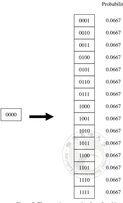
probability of pmu. If a gene set has been chosen for mutation, the proposed mutation 0001 1101 1111 1100 1011 1011 1100 1000

(16)

probability except itself. For binary-bit genes, the probability can be easily derived as

1/(2m-1), where m is the length of a gene set. Figure 3 shows an example of the

proposed mutation operation for a 4-bits gene set. Assume the gene set “0000” has

been chosen for mutation. It may be converted into one of the other 15 different gene

(17)

Note that the conventional single-point mutation operator sets a mutation rate for

each gene. That is, each gene may be mutated from 0 to 1 or vice verse according to

the given mutation rate. In this way, the probability for several neighboring genes to

simultaneously mutate will be much smaller than that for a single gene. For example,

assume the four genes “0000” are to be mutated and the mutation rate is 0.04. The 0000 0001 0010 0011 0100 0101 0110 0111 1000 1001 1010 1011 1100 1101 1110 1111 0.0667 0.0667 0.0667 0.0667 0.0667 0.0667 0.0667 0.0667 0.0667 0.0667 0.0667 0.0667 0.0667 0.0667 0.0667 Probability

(18)

fifteen possible mutation results with their probability by the conventional

single-point mutation operator are shown in Figure 4.

Note that the proposed gene-set mutation operator will assign the same 0000 0001 0010 0011 0100 0101 0110 0111 1000 1001 1010 1011 1100 1101 1110 1111 0.2349 0.2349 0.0098 0.2349 0.0098 0.0098 0.0004 0.2349 0.0098 0.0098 0.0004 0.0098 0.0004 0.0004 0.00002 Possibility

Figure 4: The probability distribution from the conventional single-point mutation operator

(19)

probability to all the possible offspring. It will thus have a larger diversity than the

conventional one.

3.3 The Proposed Gene-Set Crossover Operator

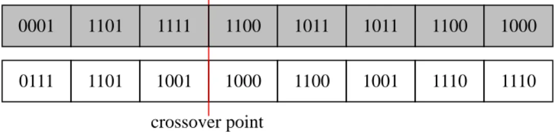
In this paper, a gene-set substring crossover operator is proposed for generating

possible offspring. The conventional substring crossover operator exchanges arbitrary

substrings between two individuals. In the proposed gene-set substring crossover

operator, the crossover points at two parents must be the same and are randomly

chosen at the boundary of gene sets. An example for the proposed gene-set crossover

operator is shown in Figure 6, where the crossover point is chosen at the end of the

third gene set. The two parent chromosomes in Figure 6(a) will crossover to produce

(20)

Note that the average length of the shorter substring in a parent chromosome by

the gene-set substring crossover operator will be a little longer than that of the

conventional one. For example in a 32-bit chromosome, the gene-set substring

crossover will set the crossover point at the boundary. There are thus seven possible

crossover points. The average length of the shorter substring for the proposed

crossover operation is calculated as (2×(4+8+12)+16)/7, which is 9.1428. The average

length of the shorter substring by the original substring crossover operation is (2×

(1+2+3+…+15)+16)/31, which is 8.2580. It is easily observed that the average length

of the shorter substring by the proposed crossover operator is longer than that by the

conventional one. The proposed crossover operator will thus in average cause wider 0001 1101 1111 1100 1011 1011 1100 1000 0111 1101 1001 1000 1100 1001 1110 1110 1100 1011 1011 1100 1000 0111 1101 1001 1000 1100 1001 1110 1110 0001 1101 1111

Figure 6: A crossover example for chromosomes with 32 bits and 4-bit genes crossover point

(a) The parent chromosomes before crossover

(21)

discrepancy between offspring and parents.

Formally, let the length of each chromosome is n and the length of each gene set

is m. When both n and m are two’s exponential expressions, the number of gene sets

will be even. In this case, the average length (AL1)of the shorter substring by the

proposed crossover operator is calculated as follows:

AL1 = [(m+2m+…+((n/2)-m)+n/2+((n/2)-m)+((n/2)-2m)+…+m)]/(n/m-1) = [2×((m+n/2-m)×((n/2)/m-1)/2)+n/2]/(n/m-1) = [(m+n/2-m)×((n/2)/m-1)+n/2]/(n/m-1) = [(n/2×((n/2)/m-1)+n/2)]/ (n/m-1) = ((n/2)2/m)/((n/m)-1) =(n/2)2/(n-m).

Similarly, the average length (AL2) by the original crossover operator is

calculated as follows: AL2 = [1+2+3+…+(n/2-1)+n/2+(n/2-1)+(n/2-2)+…+1]/(n-1) = [2×((1+n/2-1)×(n/2-1)/2)+n/2]/(n-1) = [(1+n/2-1)×(n/2-1)+n/2]/(n-1) = [n/2×(n/2-1)+n/2]/(n-1) = (n/2)2/(n-1).

(22)

Theorem: Let n be the length of each chromosome, m be the length of each gene

set. Assume n and m are two’s exponential expressions, m<n and gcd(m,n)=m. If m>1,

the average length of the shorter substring by the proposed gene-set substring

crossover operator is longer than that by the original substring crossover operator.

Proof: According to the above derivation, the average length of the shorter

substring by the proposed crossover operator is (n/2)2/(n-m), and is (n/2)2/(n-1) by the

(23)

Chapter 4 The Hierarchical Gene-Set Genetic Algorithm

A genetic process is rough when the gene-set length is large as the entire large

gene set is processed as a whole. It is thus suitable to the beginning of a genetic

process. On the contrary, the genetic process can be refined if the length is set at a

small value. A hierarchical gene-set genetic algorithm is thus proposed here to

effectively and efficiently find nearly optimal solutions to a problem. At beginning, a

larger gene-set length is set, and the genetic process is run for a fixed number of

generations (or until convergence). Then the gene-set length is shortened in half and

the genetic process is run again for a fixed number of generations (or until

convergence). The same process is repeated until the gene-set length is 1. In this way,

the proposed genetic algorithm can search more flexibly in the encoding space. A

simple example is shown in Figure 7, where the gene-set length is initially set at 4.

The genetic process for each gene-set length is run for n generations. After n

(24)

1 ~ n Generations n+1 ~ 2n Generations 2n+1 ~ 3n Generations

1011

1111

1000

1010

11 10 11 11 00 10 10 10 1 1 0 1 1 1 1 1 0 0 0 1 0 1 0 1

The proposed hierarchical gene-set algorithm is described below.

The hierarchical gene-set genetic algorithm:

INPUT: A population size P, a chromosome size w, an initial gene-set length l, a

mutation rate rm,, a crossover rate rc, and a number N of generations in each

phase.

OUTPUT: A nearly optimal solution.

Step 1: Define a suitable chromosome representation with size w for the problem to be

solved.

Step 2: Define a suitable fitness function for evaluating the individuals.

Step 3: Randomly generate a population of P individuals.

Step 4: Set k = l, where k is used to keep the gene-set length currently being Figure 7: An example for gradually adjusting gene-set length

(25)

Step 5: Set n = 1, where n is used to count the number of generations.

Step 6: Execute gene-set crossover and mutation operations on the population.

Step 8: Select the superior P individuals according to their fitness values.

Step 9: Set n = n+1.

Step 10: If n < N, repeat Steps 6 to 10; otherwise, do the next step.

Step 11: set k = k/2.

Step 12: If k < 1, stop the algorithm and output the best chromosome in the current

generation as the result; otherwise, go to Step 5.

After the process of the hierarchical gene-set genetic algorithm, a nearly optimal

(26)

Chapter 5 Theoretical Foundation for the Modified

Gene-set Genetic Algorithm

In this section, the property that a longer gene set causes a larger diversity is

formally shown. Both the crossover and the mutation operations in a long gene set

will behave better than in a short one. The derivation for the crossover operation is

first given below.

Lemma 1: Let the length of each chromosome be n and the length of each gene

set be m. When both n and m are two’s exponential expressions, the number of gene

sets will be even if n＞m, and will be 1 if n=m.

Proof: Let n=2a and m=2b, a≧b. The number of gene sets is thus 2a-b, which is

even when a＞b, and is 1 when a=b. ■

Note that in implementation, m is set smaller than n; otherwise, the gene-set

(27)

operation will generate a new totally random chromosome.

Lemma 2: Let the length of each chromosome be n and the length of each gene

set be m, n＞m. The average length (AL) of the shorter substring by the gene-set

substring crossover operator is (n/2)2/(n-m).

Proof: By Lemma 1, when n＞m, the number of gene sets is even. Thus:

AL = [(m+2m+…+((n/2)-m)+n/2+((n/2)-m)+((n/2)-2m)+…+m)]/(n/m-1) = [2×((m+n/2-m)×((n/2)/m-1)/2)+n/2]/(n/m-1) = [(m+n/2-m)×((n/2)/m-1)+n/2]/(n/m-1) = [(n/2×((n/2)/m-1)+n/2)]/ (n/m-1) = ((n/2)2/m)/((n/m)-1) = (n/2)2/(n-m). ■

Theorem 1: Let n be the length of each chromosome, and m1 and m2 be two

gene-set sizes. Assume n, m1 and m2 are all two’s exponential expressions. If m1> m2,

the average length of the shorter substring by the gene-set substring crossover

operator for m1 is longer than that for m2.

Proof: According to Lemma 2, the average length of the shorter substring by the

(28)

m2. If m1> m2, then n-m1<n-m2. Thus, (n/2)2/(n-m1) >(n/2)2/(n-m2). ■

According to Theorem 1, long gene-set sizes will get larger average substring

change by crossover operations than short ones, thus causing larger diversity. The

derivation for the mutation operation is given below.

Lemma 3: Let the length of each gene set be m, which is a two’s exponential

expression. When a gene set has been mutated, the number of all possible mutation

results is 2m-1.

Proof: When a set has been mutated, the number of combinations for the gene set to change j bits isCm_j , j≧1. The number of combinations is thus:

1 2 0 0 1 − = − =

∑

= = m m m j m j m j m j C C C . ■

Lemma 4: Let the length of each gene set be m, which is a two’s exponential

expression. When a gene set has been mutated, the average number of changed bits in

the gene set is

2 1 2 2 m m m ⋅ − .

Proof: When a gene set G has been mutated, the number of combinations for the gene set to change j bits is Cm_j , m≧j≧1. Its probability Pj is thus

(

2 −1

)

=

∑

= m m j m m k m j C C

(29)

and k=0 is excluded. Since the length m≧1, the average number of changed bits

(ACB) for G is derived as follows:

( )

(

)

(

)

(

)

(

)

(

)

(

)

(

)

(

)

⋅ = = − = = − = = ⋅ − = ⋅ ⋅ − = ⎟⎟ ⎠ ⎞ ⎜⎜ ⎝ ⎛ ⋅ − = ⎟ ⎟ ⎟ ⎠ ⎞ ⎜ ⎜ ⎜ ⎝ ⎛ ⎟ ⎠ ⎞ ⎜ ⎝ ⎛ _⋅ ₊ _⋅ − = ⎟ ⎟ ⎟ ⎠ ⎞ ⎜ ⎜ ⎜ ⎝ ⎛ ⋅ − = − ⋅ − + − ⋅ = − = − =

∑

2 1 2 2 2 2 1 2 1 2 1 2 1 2 2 1 2 1 1 2 1 1 2 1 2 1 2 / 1 2 0 2 0 2 0 2 0 0 1 m m C m C m C m C m C j m C j C j C j G ACB m m m m m j m j m m j m j m m j m m j m j m m j m m j m m m j m j m m j m j m m j ■

Lemma 5: Let two neighboring gene sets G1 and G2 exist, each with length of m,

which is two’s exponential expression. When the mutation rate for a gene set is Pm

and when at least one of the two gene sets has mutated, the conditional probability P1

for only G1 (or G2) to mutate is (1-Pm)/(2-Pm). The conditional probability P2 for both

G1 and G2 to simultaneously mutate is Pm/(2-Pm).

Proof: When the mutation rate for a gene set is Pm, the probability for only G1 to

mutate is Pm×(1- Pm), for only G2 is Pm×(1- Pm), and for both G1 and G2 is Pm×Pm.

When at least one of the two neighboring gene sets has mutated, the conditional

probability for only G1 (or only G2) to mutate is thus:

(

)

(

m

)

m

(

m

(

m

)

Pm P P P P P P P P P P P − − = + − ⋅ − = + − − 2 1 1 2 1 1 2 1 2 .

(30)

The conditional probability for both G1 and G2 to mutate is thus:

(

)

(

)

m m m m m m m m m m m P P P P P P P P P P P − = + − ⋅ ⋅ = + − 2 1 2 1 2 2 2 . ■

Lemma 6: Let two neighboring gene sets G1 and G2 exist, each with length of m,

which is two’s exponential expression. When the mutation rate for a gene set is Pm

and when at least one of the two gene sets has mutated, the average number of

changed bits in the two neighboring gene sets is

(

P

)

m m m m m m ⋅ − ⋅ ⋅ − + 1 2 2 2 2 1 2 2 2 .

Proof: When the mutation rate for a gene set is Pm and when at least one of the

two gene sets has mutated, the conditional probability for G1 (or G2) is P1, and for

both G1 and G2 is P2 according to Lemma 5. The average number of changed bits in

the two gene sets is derived as follows:

(

)

( )

(

( )

)

( )

( ) (

)

(

)

(

) (

)

(

)

(

₋

)

_⋅ ⋅ ₋ ⋅ ⋅ + = ⋅ − ⋅ + ⋅ − = ⋅ − ⋅ + ⋅ − ⋅ − ⋅ − = ⋅ − ⋅ − ⋅ − ⋅ − = ⋅ − ⋅ − + − = ⋅ − ⋅ + = ⋅ − ⋅ + = ⋅ + ⋅ = + ⋅ + ⋅ + ⋅ = + m P m P m P m P m P P P m P P m P P G ACB P G ACB P G ACB G ACB P G ACB P G ACB P G G ACB m m m m m m m m m m m m m m m m m m m m m m m m m m m m m m m m m m 1 2 2 2 2 1 2 1 2 2 2 1 2 2 1 1 2 2 2 1 2 1 2 1 2 2 2 1 1 2 2 2 1 2 1 2 2 2 1 1 2 2 2 1 1 2 2 2 1 2 2 2 2 2 2 2 2 2 2 2 2 2 2 2 2 2 1 2 1 1 2 1 1 2 1 2 2 1 1 1 2 1

(31)

■ Lemma 7: If

(

)

m m m P 2 2 1 2 ⋅ − +

﹤1 for any positive integer m ,then Pm < _m

m 2 1 2 − . Proof:

(

)

m m m P 2 2 1 2 ⋅ − + <1, Æ

(

)

m m m _P 2 2 1 2 + < − ⋅ , Æ2mP_m <2m −1, Æ _m m m P 2 1 2 − < . ■

Theorem 2: Let a gene set G of length 2m consist of two sub gene sets G1 and G2,

each with a length of m, which is a two’s exponential expression.When the mutation

rate Pm for a gene set is less than _m m

m ⋅ −1 2 2 2 2

and when the genes of length 2m has

been mutated, the average number of changed bits for 2m as a gene set unit is larger

than that for m as a gene set unit.

Proof: According to Lemma 4, the average number of changed bits for mutating

G is _m m m ⋅ −1 2 2 2 2

. According to Lemma 6, the average number of changed bits for

mutating G1 and G2 is

(

)

m P P m m m m m m _⋅ − ⋅ ⋅ − + ⋅ 1 2 2 2 2 1 2 2 2

. When Pm is less than _m

m 2 1 2 − ,

(

)

(

)

m m m m P P 2 2 1 2 ⋅ − + ⋅

﹤ 1 by Lemma 7. Thus, when Pm is less than _m

m 2 1 2 − ,

(

)

(

P

)

m P m m m m m m _⋅ − ⋅ ⋅ − + ⋅ 1 2 2 2 2 1 2 2 2 < _m m m ⋅ −1 2 2 2 2

. The average number of changed bits for 2m as

(32)

Corollary: Let m be a two’s exponential expression, when the mutation rate Pm

for a gene set is less than 0.5 and when the genes of length 2m has been mutated, the

average number of changed bits for a gene set unit of 2m is larger than that for a gene

set unit of m, m≧1.

Proof: According to Theorem 2, when Pm is less than _m

m

2 1 2 −

and when the

genes of length 2m has been mutated, the average number of changed bits for a gene

set unit of 2m is larger than that for a gene set unit of m. Since the function _m

m

2 1 2 −

is

strictly increasing and m≧1, so the minimum value of the function appears when

m=1. Thus, _m m 2 1 2 − ≦ 0.5 2 1 2 1 1 = −

. Therefore, when Pm is less than 0.5, the average

number of changed bits for a gene set unit of 2m is larger than that for a gene set unit

of m, m≧1. ■ Lemma 8: When Pm1> Pm2,

(

)

(

)

(

)

n

)

m m n m m P P P P 2 2 1 1 1 1 1 1− − > − − for anyn≧2.

Proof: We use the mathematical induction to prove it. When n=2, the following

formulas hold:

(

)

(

)

(

) (

2

)

2 2 2 1 1 2 2 1 2 1 2 1 1 1 2 1 1 2 2 2 2 1 1 m m m m m m m m m m m m m P P P P P P P P P P P P P − ⋅ − − = − = − − , and

(

)

(

)

(

) (

2

)

2 2 2 1 1 2 2 1 2 1 2 2 2 2 2 2 2 2 2 2 2 1 1 m m m m m m m m m m m m m P P P P P P P P P P P P P − ⋅ − − = − = − − .

(33)

When Pm1> Pm2, P_m₁P_m2₂ =P_m₁P_m₂P_m₂ <P_m₁P_m₁P_m₂ =P_m2₁P_m₂. Thus,

(

) (

2

)

2 2 2 1 1 2 2 1 2 1 2 2 2 2 1 1 2 2 1 2 1 2 2 2 2 2 2 m m m m m m m m m m m m m m m m P P P P P P P P P P P P P P P P − ⋅ − − > − ⋅ − − .

Then we assume the conclusion holds for n = k and prove that it will also hold

for n = k+1. Thus when n = k, the following formula holds:

(

)

(

)

(

)

k

)

m m k m m P P P P 2 2 1 1 1 1 1 1− − > − − . It implies P_m1−P_m1⋅

(

1−P_m2

)

k >P_m2 −P_m2⋅

(

1−P_m1

)

k.

The following formula can be derived for n = k+1:

(

)

(

)

(

)

(

)

(

)

(

)

(

)

(

) (

(

)

1

)

2 1 1 2 2 1 1 1 2 1 1 1 2 1 1 1 1 1 1 1 1 1 . 1 1 1 1 1 1 1 1 1 + + + + + + ₋ ₋ _⋅ ₋ ₋ − − − = − − ⋅ − − − − = − − k m k m m k m m m k m k m k m m k m m P P P P P P P P P P P P

(

)

(

)

(

)

(

)

(

)

1

)

2 1 1 2 2 1 2 1 1 1 1 1 1 1 1 + + _⋅ ₋ ₋ − − − + − − = _k m k m k m m m k m m m P P P P P P P P . Similarly,

(

)

(

)

(

)

(

)

1

)

2 1 1 1 2 1 1 2 2 1 2 2 1 1 1 1 1 1 1 1 + − − + ⋅ − − + − + − − = − − k m k m k m m m k m m m k m m P P P P P P P P P P .

When Pm1> Pm2, the following formulas can hold fork >1:

(

)

(

)

k m m m k m m m P P P P P P 1− 1 1− 2 > 2 − 2 1− 1 , and

(

)

(

)

k m m m k m m m P P P P P P 1 2 1− 2 > 1 2 1− 1 . Thus,

(

)

(

)

(

)

(

)

(

)

(

)

(

)

1

)

2 1 1 1 2 1 1 2 2 1 2 1 1 2 2 1 2 1 1 1 1 1 1 1 1 1 1 1 1 1 1 + + + + ₋ ₋ _⋅ ₋ ₋ − + − − > − − ⋅ − − − + − − k m k m k m m m k m m m k m k m k m m m k m m m P P P P P P P P P P P P P P P P . It implies

(

)

(

)

(

)

1

)

2 1 1 1 1 1 1− − + > − − k+ m k m P P P P .

(34)

Thus according to the mathematical induction, when Pm1>Pm2, the following

inequality holds any n≧2.

(

)

(

)

(

)

n

)

m m n m m P P P P 2 2 1 1 1 1 1 1− − > − − . ■

Lemma 9: Let a gene set G consist of n sub gene sets, n≧2. When the gene set

is mutated by the gene-set mutation operator according to the sub-gene-set size, the

average number of mutated sub gene sets with mutation rate Pm1 is larger than that

with Pm2 if Pm1> Pm2.

Proof: When a gene set G is mutated with the mutation rate Pm1 by the gene-set

mutation operator, the conditional possibility for a sub gene set to mutate is Pm1/(1-(1-

Pm1)n). Its average number of mutated sub gene sets is

(

)

(

n

)

m m P P n 1 1 1 1− − × . Similarly,

the average number of mutated sub gene sets with the mutation rate Pm2 is

(

)

(

n

)

m m P P n 2 2 1 1− − × . When Pm1>Pm2,

(

)

(

)

(

)

n

)

m m n m m P P P P 2 2 1 1 1 1 1 1− − > − − for any n≧2

according to Lemma 8. Thus, when the gene set is mutated by the gene-set mutation

operator according to the sub-gene-set size, the average number of mutated sub gene

sets with mutation rate Pm1 is larger than that with Pm2 if Pm1> Pm2. ■

Theorem 3: Let a gene set G of length m consist of n sub gene sets, each with

(35)

a gene set to mutate is less than 0.5 and when the gene set G has been mutated, the

average number of changed bits for mutating G is larger than that for mutating sub

gene sets.

Proof: When the mutation rate Pm is set at 0.5, the probability of mutating a

certain group of k sub gene sets is 0.5x(1-0.5)n-x , which is equal to 0.5n. The

probability of mutating any arbitrary group of sub gene sets is thus the same for Pm =

0.5. When the gene set G has been mutated, the number of combinations for j sub

gene sets to be mutated is Cm_j , j≧1. Its probability Pj is ( (2 1))

1 − =

∑

= n n j n k n k n j C C C ,

where k starts from 1 since the gene set has been mutated and k=0 has been excluded.

When n>1, the average number of mutated sub gene sets is derived as follows:

(

)

(

)

(

)

(

)

(

)

(

)

(

)

(

)

⋅ = = − = = − = ⋅ − = ⋅ ⋅ − = ⎟⎟ ⎠ ⎞ ⎜⎜ ⎝ ⎛ ⋅ − = ⎟ ⎟ ⎟ ⎠ ⎞ ⎜ ⎜ ⎜ ⎝ ⎛ ⎟ ⎠ ⎞ ⎜ ⎝ ⎛ _⋅ ₊ _⋅ − = ⎟ ⎟ ⎟ ⎠ ⎞ ⎜ ⎜ ⎜ ⎝ ⎛ ⋅ − = − ⋅ − + − ⋅ = −

∑

2 1 2 2 2 2 1 2 1 2 1 2 1 2 2 1 2 1 1 2 1 1 2 1 2 1 2 0 2 0 2 0 2 0 1 n n C n C n C n C n C j n C j C j n n n n n j n j n n j n j n n j n n j n j n n j n n j n n n j n j n n j

According to Lemma 4, when a sub gene set has been mutated, the average

number of changed bits in the sub gene set is

2 1 2 2 z z z ⋅

− . Thus, the average number of changed bits in the mutated n sub gene sets is )

2 1 2 2 ( ) 2 1 2 2 ( n _z z z n n ⋅ − ⋅ ⋅ − , which is 1 2 2 1 2 2 4 ⋅ − ⋅ z − z n n m . Since both 1 2 2 − n n and 1 2 2 − z z

are strictly decreasing for positive

(36)

the mutated n sub gene sets is thus less than , 1 2 2 1 2 2 4 1 1 2 2 − ⋅ − ⋅ m which is ) 3 2 ( 1 2 3 4 4 m m_⋅ _⋅ ₌

. Besides, the average number of changed bits for mutating G is

2 1 2 2 m m m ⋅

− according to Lemma 4. Since 2 1 2 2 3 2m m m m ⋅ −

≤ for m≧2, the average

number of changed bits for mutating G is larger than that for mutating n sub gene sets

when the mutation rate is set at 0.5.

According to Lemma 9, if the mutation rate is less than 0.5, the average number

of mutated sub gene sets is less than

⋅ ⋅ − 21 2 2 n n n

. It implies that the average number of

changed bits is less than )

2 1 2 2 ( ) 2 1 2 2 ( n _z z z n n ⋅ − ⋅ ⋅ − , which is equal to 1 2 2 1 2 2 4 ⋅ − ⋅ z − z n n m

. Thus, when the mutation rate Pm for a gene set is less than 0.5 and

when the gene set G has been mutated, the average number of changed bits for

mutating G is larger than that for mutating n sub gene sets. ■

From the above theorems, it can be seen that when a mutation or crossover

operator has been performed, using a longer gene set can cause more bits to be

changed than using a shorter one. The former can thus generate more different

(37)

Chapter 6 A Modified Gene-Set Genetic Algorithm

When a population converges, the solutions may be local optimal or global

optimal. Although the mutation operation can be used to help the genetic process

escape from local optimums, the escape speed is slow and depends on the mutation

rate. As mentioned above, the gene sets with a larger length will have larger variation.

This characteristic will be used here to speed up escape from local optima.

The escape operator based on this characteristic can easily be designed as fallows.

Let the current gene-set length is m. If the genetic process for the length has

converged, but has not gotten to the assigned number of generations, the gene-set

length will be changed to a value bigger than m. The above escape operator, when

used together with the other genetic operators, will thus cause a large variation to help

a population escape from local optima. The escape operator is performed when the

best solutions in the current population converge. The gene-set crossover and

mutation processes are then run for the enlarged gene-set length for only one

generation. After that, it is run for the original length until the best solutions converge.

(38)

predefined number of generations is achieved. The next genetic phase for a half

gene-set length then begins. Before the proposed algorithm is described in detail, the

concept of (δ, k)-converging is defined below.

Definition: (δ, k)-converging - Let δ>0 and best(r) be the best solution in the

population of the r-th generation. The r-th generation is called (δ, k)-converging if and

only if |best(r)– best(r–z+1)|≦δ for every z≦k.

When a generation is (δ, k)-converging, the best solution in that generation has

not been improved in recent k generations. Two possible situations may exist. One is

the global optimal solution has been found, and the other is the population has lost its

variety and has been trapped into local optima. The above escape operation will be

integrated in the proposed algorithm to avoid the occurrence of the latter situation.

The modified gene-set genetic algorithm with escape operation is described below.

The modified gene-set genetic algorithm with escape operation:

INPUT: A population size P, a chromosome size n, an initial gene-set length l1, a

mutation rate rm,, a crossover rate rc, an enlarged gene-set length l2 for escape

operation, a number N of generations in each phase, and two parameters δ

(39)

Step 1: Define a suitable chromosome representation with size n for the problem to be

solved.

Step 4: Set l = l1, where l is used to keep the gene-set length currently being

processed.

Step 5: Set g = 1, where g is used to count the number of generations.

Step 6: Execute the gene-set crossover and mutation operations on the population.

Step 8: Select the superior P individuals according to their fitness values.

Step 9: Set g = g+1.

Step 10: If g < N and the current generation is not (δ, k)-converging, go to Step 6.

Step 11: If g < N and the current generation is (δ, k)-converging, do the escape

operation as follows:

Substep 11-1: Set temp = l, where temp is used to keep the current gene-set

length.

Substep 11-2: Set the gene-set length l = l2.

Substep 11-3: Execute the gene-set crossover and mutation operations for

(40)

Substep 11-4: Set g = g+1.

Substep 11-5: Set l = temp.

Substep 11-6: Go to Step 6.

Step 12: If g = N, set l = l/2.

Step 13: If l < 1, stop the algorithm and output the best chromosome in the current

generation as the result; otherwise, go to Step 5 for the next genetic phase.

After the process of the modified gene-set genetic algorithm, a nearly optimal

solution to the given problem can be found. Using the escape operation, the proposed

algorithm can help the escape of local optima through the change of gene-set sizes to

a large value. Even when the population has (δ, k)-converged, the proposed algorithm

can also help the search of global optima since the gene-set operations with the

original gene-set length will still be done as long as the predefined number of

termination generations is not achieved. The modified gene-set genetic algorithm can

(41)

Chapter 7 Theoretical Foundation for the Modified

Gene-set Genetic Algorithm with Dynamic

Mutation Rates

In this section, the property that using longer gene sets will cause the population

to produce less offspring is formally shown. The derivation is given below.

Lemma 1: Let a chromosome S of length m consist of m/n gene sets of length n,

m/n is an integer. When the mutation rate is Pm, the probability of a chromosome which is mutated is 1-(1- Pm)m/n.

Proof: When the mutation rate is Pm, the probability for a gene set not to mutate

is (1- Pm). Thus the probability for all the gene sets in the chromosome S not to mutate

is (1- Pm)m/n. The probability for the chromosome S to mutate is 1-(1-Pm)m/n. ■

Lemma 2: Let a population P consist of x chromosomes of length m, each of

(42)

is Pm, the expected value of the number of offspring produced from P by mutation is x

×(1-(1- Pm)m/n).

Proof: According to Lemma 1, the probability of a chromosome which is

mutated is 1-(1- Pm)m/n. Thus, the expected value of the number of offspring produced

from P by the mutation operator is x×(1-(1- Pm)m/n). ■

Theorem 1: Let there be two populations P1 and P2, each of which consists of x

chromosomes of length m. Assume each chromosome in P1 consists of m/n1 gene sets

of length n1, and each chromosome in P2 consists of m/n2 gene sets of length n2, where

m/n1 and m/n2 are integers. When the mutation rate is Pm and n1 > n2, P1 will in

average produce less offspring than P2 by the gene-set mutation operator.

Proof: According to Lemma 2, the expected value of the number of offspring

from P1 by the gene-set mutation operator is x×(1-(1- Pm)m/n1), and from P2 is x×(1-(1-

Pm)m/n2). When n1 > n2, it can be derived that m/n1 < m/n2 and x×(1-(1-Pm)m/n1) < x×

(1-(1-Pm)m/n2). P1 will thus in average produce less offspring than P2 by the gene-set

mutation operator. ■

From the above theorem, it can be concluded that using longer gene sets will

(43)

be allowed larger mutation rates, thus being able to mend the shortcoming of the

(44)

Chapter 8 A Modified Gene-Set Genetic Algorithm with

Dynamic Mutation Rates

When a population converges, the solutions may be local optimal or global

optimal. Although the mutation operation can be used to help the genetic process

escape from local optimums, the escape speed is slow and depends on the mutation

rate. As mentioned above, the gene sets with a larger length will have larger variation.

An escape operator based on this characteristic can easily be designed as fallows. Let

the current gene-set length is m. If the genetic process for the length has converged,

but has not gotten to the assigned number of generations, the gene-set length will be

changed to a value bigger than m. The above escape operator, when used together

with the other genetic operators, will thus cause a large variation to help a population

escape from local optima. The escape operator is performed when the best solutions in

the current population converge. The gene-set crossover and mutation processes are

then run for the enlarged gene-set length for only one generation. After that, it is run

(45)

enlarged again. The above process is repeated until the predefined number of

generations is achieved. The next genetic phase for a half gene-set length then begins.

In addition, from the above theorem, using longer gene sets will cause a

population to produce less offspring. Longer gene sets will thus be allowed larger

mutation rates, thus being able to amend the shortcoming of the generated offspring

due to the longer gene-set size and evolve better solutions. There are thus two

principles for adjusting the mutation rates to be followed. The first one is that the

mutation rate at a longer gene set is larger than that at a smaller one; the second one is

that all the mutation rates can not be set too large to guarantee the performance

becomes poorer than that by the simple GA. In this paper, the proposed algorithm will

simultaneously consider the escape operation and the dynamic mutation rate to

effectively help the escape of local optimums.

The modified gene-set genetic algorithm with the escape operation and dynamic

mutation rates is described below.

The modified gene-set genetic algorithm with dynamic mutation rates:

INPUT: A population size P, a chromosome size n, an initial gene-set length l1, an

(46)

generations in each phase, and two parameters δ and k.

OUTPUT: A nearly optimal solution.

Step 1: Define a suitable chromosome representation with size n for the problem to be

solved.

Step 4: Set l = l1, where l is used to keep the gene-set length currently being

processed.

Step 5: Set g = 1, where g is used to count the number of generations.

Step 6: Execute the gene-set crossover and mutation operations on the population

using the crossover rate rc and the mutation rate rmt for the gene-set length of

t.

Step 8: Execute the selection mechanism to generate the next population.

Step 9: Set g = g+1.

Step 10: If g < N and the current generation is not (δ, k)-converging, go to Step 6.

Step 11: If g < N and the current generation is (δ, k)-converging, do the escape

(47)

Substep 11-1: Set temp = l, where temp is used to keep the current gene-set

length.

Substep 11-2: Set the gene-set length l = l2.

Substep 11-3: Execute the gene-set crossover and mutation operations on the

population using the crossover rate rc and the mutation rate

rml for the gene-set length l. Substep 11-4: Set g = g+1.

Substep 11-5: Set l = temp.

Substep 11-6: Go to Step 6.

Step 12: If g = N, set l = l/2.

Step 13: If l < 1, stop the algorithm and output the best chromosome in the current

generation as the result; otherwise, go to Step 5 for the next genetic phase.

After the process of the modified gene-set genetic algorithm with dynamic

mutation rates, a nearly optimal solution to the given problem can be found. Using the

escape operation, the proposed algorithm can help the escape of local optima through

the change of gene-set sizes to a large value. Using dynamic mutation rates, the

proposed algorithm can enlarge the searching region to amend the shortcoming of the

(48)

(49)

Chapter 9 Experimental Results

This section reports on experiments made to show the performance of the

proposed genetic algorithm. They were implemented in C Language on an AMD K7

2200+ with the Linux OS. Also presented are experiments made to compare the time

required by the proposed genetic algorithm and by the simple genetic algorithm. The

following three problems were used for test:

(A) f_A

( ) (

x =−350−x

)

2 +500, find the maximum;

(B) f_B

( ) (

x = x−2.6

) (

× −19−x

) (

× x+56.5

) (

× x−3

)

, find the maximum;

(C) f_C

( )

x = x4×sin

(

2xπ

)

for 0 < x < 100, find the maximum.

The first function is a simple one-peak function with only one local (also global)

optimal solution. The second one has two peaks, and the third one has multiple peaks.

In all the experiments, the chromosome length was 32 and the initial gene-set length

was 4. The termination criterion was the generation number, with each phase being

(50)

Experiments were first made for Function A. The problem could actually be

solved by calculus. It was used here to compare the performance of the modified

approach and the others. The population size was set at 100 and the total generation

number was set at 2100 (each phase had 700 generations). When the mutation rates

were set at 0.06, 0.08, 0.1 and 0.32 respectively for the gene-set length of 1, 2, 4 and

16, the relation between fitness values and generations for Function A is shown in

Figure 8, where SGA represents simple GA, HGSGA represents the gene-set SGA

without the escape operation, HGSGA(m) represents the modified HGSGA with the

escape operation, and HGSGA(m2) represents the modified HGSGA with the escape

operation and dynamic mutation rates.

Population size: 100, Mutation rate: 0.06, Function A

-10000 -8000 -6000 -4000 -2000 0 2000 0 300 600 900 1200 1500 1800 2100 2400 generations fi tn es s va lu e

(51)

Figure 8: The fitness values along with different generations for Function A.

It can be observed from Figure 4 that the fitness values by all the four

approaches increased along with the increase of generations. It was quite consistent

with the characteristics of GAs. Besides, the gene-set genetic algorithms performed

better than SGA and the proposed gene-set genetic algorithm with dynamic mutation

rates performs best among the four. It can find the global optimal solution very fast.

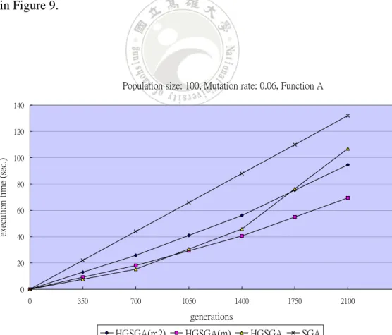
The execution time along with generations by the four algorithms for Function A is

shown in Figure 9.

0 20 40 60 80 100 120 140 0 350 700 1050 1400 1750 2100 generations execut ion time ( sec.)

(52)

It can be seen from Figure 9 that the gene-set genetic algorithms needed less

computational time than SGA. HGSGA(m) could even spend less computational time

than HGSGA due to the escape operations. HGSGA(m2) spent a little more

computational time than HGSGA(m) since the former might generate more offspring

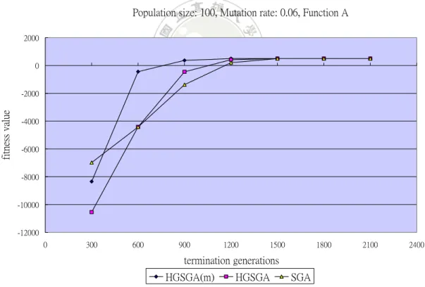
to process. Experiments were then made for showing the relations between fitness

values and termination generations. For mutation rate set at 0.06, the results for

Function A are shown in Figure 10.

-12000 -10000 -8000 -6000 -4000 -2000 0 2000 0 300 600 900 1200 1500 1800 2100 2400 termination generations fitne ss va lue

HGSGA(m) HGSGA SGA

Figure 10: The fitness values along with different termination generations for

(53)

It can be observed from Figure 10 that the fitness values by all the three

algorithms increased along with the increase of termination generations. When the

number of termination generations was small, convergence could not be achieved.

The gene-set genetic algorithms had a worse effect than SGA since the former ran

only 1/3 of total generations for each phase. But along with the number of termination

generations increased, HGSGA and HGSGA(m) generated better fitness values than

SGA. Besides, HGSGA(m) is better than HGSGA. The execution time along with the

number of termination generations for Function A by the three algorithms is shown in

(54)

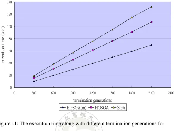
Population size: 100, Mutation rate: 0.06, Function A 0 20 40 60 80 100 120 140 0 300 600 900 1200 1500 1800 2100 2400 termination generations ex ec utio n tim e (s ec .)

HGSGA(m) HGSGA SGA

Figure 11: The execution time along with different termination generations for

Function A.

It can be seen from Figure 7 that HGSGA(m) needed the least computational

time among the three algorithms for different termination generations. Next,

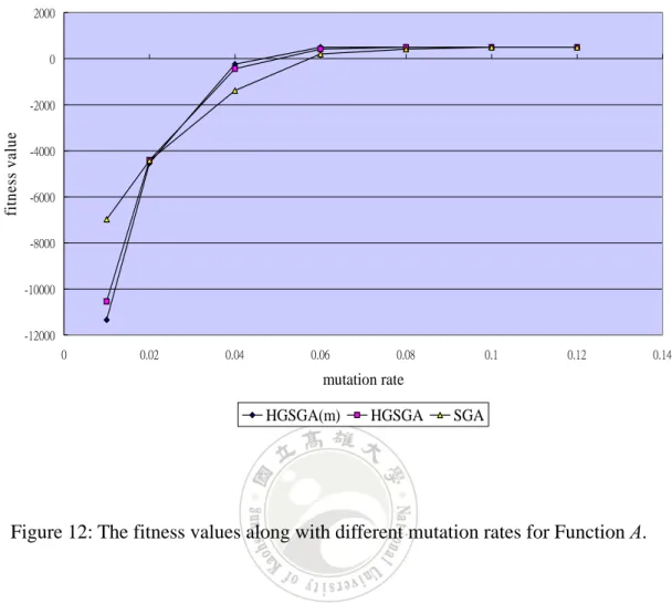
experiments were made to show the effect of the mutation rate on the proposed

algorithm. The genetic process was terminated at 600 generations. The final best

fitness values along with different mutation rates for Function A by the three

(55)

Population: 100, Generation: 600, Function A -12000 -10000 -8000 -6000 -4000 -2000 0 2000 0 0.02 0.04 0.06 0.08 0.1 0.12 0.14 mutation rate fitn es s v alu e

HGSGA(m) HGSGA SGA

Figure 12: The fitness values along with different mutation rates for Function A.

It can be observed from Figure 12 that the fitness value increased along with the

increase of the mutation rates when the rates where lets then 0.12. Mutation rates were

thus very important to the final results of the algorithms. From the above experimental

results, the modified approach needed a higher number of generations and a higher

mutation rate to achieve a better performance. Experimental results for Function B are

(56)

Population size: 100, Mutation rate: 0.06, Function B 400000 450000 500000 550000 600000 650000 700000 0 300 600 900 1200 1500 1800 2100 2400 generations fi tn es s va lu e

HGSGA(m2) HGSGA(m) HGSGA SGA

(57)

Population size: 100, Mutation rate: 0.06, Function B 0 20 40 60 80 100 120 140 0 350 700 1050 1400 1750 2100 generations ex ec ut io n ti m e (s ec .)

HGSGA(m2) HGSGA(m) HGSGA SGA

Figure 14: The execution time along with different generations for Function B

Note that in Figure 13, the gene-set sizes in the HGSGA and HGSGA(m) were

long at the beginning generations, which were regarded as a rough optimization phase.

In this phase, the offspring generated by the two gene-set algorithms lacked delicate

local search but focused on big escape movement. The fitness of HGSGA and

HGSGA(m) was thus worse than that of SGA in this phase. Along with the gene-set

size becoming smaller, the local search in HGSGA and HGSGA(m) were performed

more and more delicately and the escape effect was still better than that in simple GA.

(58)

help search in the solution space, such that its fitness was better than the other

algorithms in each generation.

Population size: 100, Mutation rate: 0.06, Function B

400000 450000 500000 550000 600000 650000 700000 0 300 600 900 1200 1500 1800 2100 2400 termination generations fi tn es s va lu e

HGSGA(m) HGSGA SGA

Figure 15: The fitness values along with different termination generations for

(59)

Population size: 100, Mutation rate: 0.06, Function B 0 20 40 60 80 100 120 140 0 300 600 900 1200 1500 1800 2100 2400 termination generations ex ec ut io n ti m e (s ec. ) HGSGA(m) HGSGA GA

Figure 16: The execution time along with different termination generations for