Originals Experiments in Fluids 24 (1998) 373—374( Springer-Verlag 1998
An artificial neural network for double exposure PIV image analysis
P.-H. Chen, J.-Y. Yen, J.-L. Chen
Abstract This note presents a back propagation neural network for PIV image analysis. Unlike the conventional auto-correlation method that identifies one pair of image out of the picture, the proposed network distinguishes all the image pairs in the measurement area and provides different labels for each pair. Experimental investigations show good agreement with the auto-correlation process for the uniform flow mea-surement, and a 78.1% success ratio for the stagnation flow.
1
Introduction
This note investigates the use of a neural network for a double exposure particle image velocimetry (PIV) flow field analysis. The PIV system uses a two-dimensional auto-correlation process to infer a proper pair from among the particle images recorded on a photographic film (Adrian 1991). Although the auto-correlation process involves very intensive computation, and it requires the assumption that the flow has to be fairly uniform (Anderson and Longmire 1996), little improvements have been made. Most popular modifications seek to introduce interpolation and extrapolation to widen its applications. There is also an attempt to aid the analysis with the Particle Tracking Velocimetry (PTV) technique, which is a redundant practice limited by the equipment complexity (Anderson and Longmire).
An alternative to the auto-correlation process to perform image pairing is to use the artificial neural network (Grant and Pan 1995; Carosone et al. 1995). The former results claim 60—97% success ratio depending on different degrees of flow turbulence and image densities. In this note, the authors try to develop a more universal neural network for image pairing in the PIV system. Unlike the former network which identifies one pair of particles in each ‘‘segment’’, the proposed network takes all the input information simultaneously and attaches separate labels to all the distinguishable image pairs. The experimental results show that the proposed network achieves a good success ratio, and is capable of velocity vectors in
Received:9January1997/Accepted:10September1997 P.-H. Chen, J.-Y. Yen and J.-L. Chen
Department of Mechanical Engineering, National Taiwan University, Taipei, Taiwan 10764, R.O.C.
Correspondence to: J.-Y. Yen
relatively diverse directions. Thus, the uniform flow field assumption for the two-dimensional auto-correlation process is also somewhat relaxed.
2
The neural network for PIV image analysis
The PIV system shines two consecutive sheets of laser pulses into the fluid flow and records the scattered particle images on a photographic film. As a result, each particle will leave two images on the film, and the distance between these images and the relative positions determines the two-dimensional velocity vector. The resolution for the 1 mm2 PIV interrogation area is 512]512 pixels. For a good average velocity, this picture is first reduced to 32]32 pixels, and the neural network processes a quarter picture, which are 16]16 pixels, at a time. To improve the velocity estimation, the center of each particle image is computed and recorded before the reduction.
To avoid ambiguity, the gray levels are thresh-held to 0 and 1, where a 1 would represent the appearance of a particle center. The centers of the particles are calculated by averaging the four edges of the images. Since the pictures are 512]512 pixels, the measurement resolution for distance is 2lm.
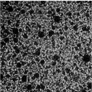
Fig. 1. The PIV image of the flow in front of a moving turbine blade
Fig. 2. The PIV neural network pairing result for Fig. 1
The output value for the output layer would be zero if the corresponding input value is zero. The same output value would appear to the output neurons corresponding to the images in the same pair. To distinguish image pairs from different parent particle, different output values are assigned to different pairs to distinguish different parent particles. In this note, the locations close to the upper left corner are assigned values close to 1, and the locations close to the lower right corners are assigned with values close to 0. The distribution from 0 to 1 is more or less even. The output values are normalized so that they distribute evenly from 0 to 1. There are 257 neurons for the input layer. The first 256 neurons contain the discrete gray level. The last neuron is used for noise handling. The value is set to be[1. The hidden layer is decided to be 120 neurons. The output layer contains 256 neurons. To make analysis easier, the transfer functions for the neurons use a uni-polar function so that the outputs are always positive. Usually, an additional filter is used to add a thresh-hold above 0.02 and round off to the second digit on the results. The learning process follows the standard back propagation network. Each learning cycle contain 16 training pictures. The learning error is accumulated for all 16 examples. Thus, the resultant learning error is accumulated for all the processes. In this application, the error converges in around 60 iterations.
3
Neural network PIV measurement result and discussions
Figure 1 shows as an example a PIV picture taken by the system. The picture is the result of a CID picture in front of a moving turbine blade. Figure 2 is the neural network pairing result for the upper-right quarter of the picture. There are clearly 4 pairs of distinguishable images valued at 0.0805, 0.1305, 0.7224 and 0.9559. The rest of the images could be a result of the parting process with left over images, and the thresh-holding process that took out blurred images. From the results of the neural network identification, there are 16 pairs of distinguishable particle images on the picture. The average horizontal distance between the images is 53.87 pixels which is
equivalent to 0.10521 mm. The average vertical distance is 0.01 pixels which is 0.00002 mm. Therefore, the horizontal velocity component is 0.5845 mm/sec and the vertical velocity com-ponent is 0.0001 mm/sec. The auto-correlation process gives horizontal velocity 0.5627 mm/s, and vertical velocity 0.000103 mm/s. There is a 3.13% difference between the results. It is not clear at present which result is more accurate. This will be a topic for further research.
4
Conclusions
This paper presents a back propagation neural network for the PIV image pairing. Unlike the former auto-correlation pro-cess and the other neural network approaches that try to single out one average image displacement for velocity estimation, the proposed network identifies all the distinguishable pairs of images and provides clear labels for each image pair. The average velocity is then derived from the average of the velocities of all the resultant image pairs. The experimental results show that the proposed network works very well in measuring uniform flow field velocity. The success ratio for the stagnation flow field identification is 78.1%. It is not clear at this point if the auto-correlation process provides more accurate measurement results than the neural network. Since the network is not trained for diverse flow pattern, the authors also believe that the neural network can achieve better identification results in turbulent flow measurement.
References
Adrian RJ(1991) Partical-imaging techniques for experimental fluid mechanics. Annu Rev Fluid Mech 23: 261—304
Anderson SL; Longmire EK(1996) Interpretation of PIV auto-correlation measurements in complex particle-laden flows. Exp Fluids 20: 314—317
Grant I; Pan X(1995) An investigation of the performance of multi-layer, neural networks applied to the analysis of PIV images. Exp Fluids 19: 159—166
Carosone F; Cenedese A; Querzoli G(1995) Recognition of partially overlapped particle images using the kohonen neural network. Exp Fluids 19: 225—232