高車速下多輸入多輸出正交分頻多工系統中結合資料偵測及通道估計之遞迴式接收機架構

國 立 交 通 大 學

電信工程學系

碩 士 論 文

高車速下多輸入多輸出正交分頻多工系統中

結合資料偵測及通道估計之遞迴式接收機架構

An Iterative Receiver Architecture Based on Joint Data

Detection and Channel Estimation for High Mobility

MIMO OFDM Systems

研究生：李思潔

指導教授：黃家齊 博士

高車速下多輸入多輸出正交分頻多工系統中

結合資料偵測及通道估計之遞迴式接收機架構

An Iterative Receiver Architecture Based on Joint Data Detection and

Channel Estimation for High Mobility MIMO OFDM Systems

研 究 生：李思潔 Student：Sih-Jie Li

指導教授：黃家齊 博士 Advisor：Dr. Chia-Chi Huang

國 立 交 通 大 學

電信工程學系

碩 士 論 文

A Thesis

Submitted to Department of Communication Engineering College of Electrical and Computer Engineering

National Chiao Tung University in partial Fulfillment of the Requirements

for the Degree of Master of Science

in

Communication Engineering August 2008

Hsinchu, Taiwan, Republic of China

高車速下多輸入多輸出正交分頻多工系統中

結合資料偵測及通道估計之遞迴式接收機架構

學生：李思潔

指導教授：黃家齊博士

國立交通大學電信工程學系 碩士班

摘

要

對於應用於高移動通訊環境之正交分頻多工(Orthogonal Frequency

Division Multiplexing, OFDM)系統，每一個 OFDM 符元期間的通道時變導

致載波間干擾(Inter-carrier Interference, ICI)發生，使得系統效能降低。當載

具速度、OFDM 符元期間增加，影響將更為嚴重。在這篇論文中，針對高

移動性無線通道下之多輸入多輸出(MIMO) OFDM 系統，我們提出一個基於

結合通道估計與資料偵測之遞迴式接收機架構，此架構主要由三級程序組

成。在初始級，我們採用多重路徑干擾消除方法來粗略估計多重路徑延遲

及多重路徑複數增益等通道參數；在追蹤級，我們先使用一個β-追蹤器，

之後再使用基於 V-BLAST 資料偵測之決策迴授離散傅立葉轉換通道估測

方式，以估計每條路徑的增益平均值；在最後一級中，我們採用一個線性

模型來近似每條路徑的時域變化，然後再利用一個二維的 V-BLAST 方法做

資料決策，來達到消除 ICI 效應的目的。最後，我們以電腦模擬結果驗證了

此遞迴式接收機在高移動性通道的效能增進。

An Iterative Receiver Architecture Based on Joint Data Detection

and Channel Estimation for High Mobility MIMO OFDM Systems

Student：Sih-Jie Li

Advisors：Dr. Chia-Chi Huang

Department of

Communication Engineering

National Chiao Tung University

ABSTRACT

For orthogonal frequency division multiplexing (OFDM) systems in high-mobility environment, channel variations within one OFDM symbol will introduce intercarrier interference (ICI), thus lowering the system performance. This becomes more severe as vehicle speed or OFDM symbol duration increase. In this paper, an iterative receiver architecture based on joint channel estimation and data detection is proposed for MIMO OFDM systems in mobile wireless channels. The iterative receiver mainly consists of three-stage processing. In the initialization stage, we employ a multipath interference cancellation technique to roughly estimate multipath delays and multipath complex gains through the preamble. In the tracking stage, a

β

-tracker is applied first, followed by decision-feedback (DF) DFT-based channel estimation which is based on V-BLAST data detection, so as to estimate the average channel variations of each path. In the final stage, we adopt a linear model to approximate time variations of each path, and a two-dimensional V-BLAST method is utilized to perform ICI cancellation and data detection. Finally, computer simulations are conducted to verify the performance of the iterative receiver in high-mobility channels.

誌

謝

感謝指導教授黃家齊老師對於我研究和學業上的指導與勉勵，給予我

待人處事上的最佳模範。感謝老師在我研究所的兩年裡的指導與包容，使

我在兩年的研究所生涯中獲益匪淺。感謝口試委員黃正光教授及陳紹基教

授對本篇論文的指導與意見。

特別感謝博士班的古孟霖學長，在研究方面給予我莫大的幫助。在我

研究上有困難時，不厭其煩地教導與關心，對我提出的任何疑問，都能耐

心解說，使我得以順利完成論文。與學長的討論常使我收穫良多，學長的

研究態度更是我的最好榜樣。

感謝冠群、小汪一直以來對我的照顧和生活上各方面的幫助，以及與

人豪一起為實驗室電腦的維護。與你們的相處，輕鬆愉悅又不失溫馨，讓

我度過這一段快樂時光。也感謝同屆同學阿威、文娟、建勳和學弟妹王森、

曉顗以及實驗室所有成員的相互勉勵和關心。

最後，感謝我的家人，給予我精神上的鼓勵與支持，你們一直是支持

我走下去的動力。

Contents

中文摘要 ... i  ABSTRACT ... ii  誌謝 ... iii  Contents ... iv  List of Figures ... v  Chapter 1  Introduction ... 1 

Chapter 2  MIMO OFDM System ... 5 

2.1  Transmitted Signals ... 5 

2.2  Channel Model ... 7 

2.3  Received Signals ... 7 

2.4  ICI on OFDM System ... 8 

Chapter 3  V-BLAST Detection ... 11 

Chapter 4  Iterative Receiver ... 16 

4.1  Initialization Stage: The MPIC-Based Decorrelation Method ... 17 

β

-tracker ... 19 

4.2  Tracking Stage: 4.3  ICI Estimation ... 27 

4.4  Two Dimensional V-BLAST Detection ... 33 

Chapter 5  Performance Simulation ... 36 

5.1  System Parameters ... 36 

5.2  Simulation Results ... 37 

Chapter 6  Conclusions ... 48 

List of Figures

Fig. 1 MIMO OFDM system ... 5  Fig. 2 OFDM frame format ... 5  Fig. 3 Block diagram of the channel estimation in the tracking stage and the ICI cancellation

in the final stage. ... 16  Fig. 4 The MPIC-based decorrelation method in the initialization stage ... 19  Fig. 5

β

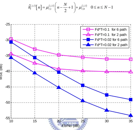
-tracker followed by DF DFT-based channel estimation method in the tracking stage

... 26  Fig. 6 NMSE of the channel estimation with the assumption that the average channel

variations μ_l( )_,0j i, 0,for l= …,L( )j i, _b/ _o . A frequency F frequency F frequency F frequency F * d F T at E_b/N_o=25d frequency F frequency F

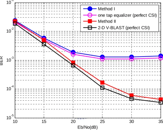
are known versus E N ... 32  Fig. 7 ICI effect from neighboring subcarriers with group size ... 34  Fig. 8 BER performance in the two-path channel for normalized Doppler

* =0.02

d T ... 41 

Fig. 9 BER performance in the ITU Veh-B channel for normalized Doppler * =0.02

d T ... 42 

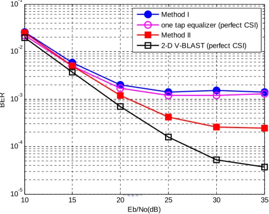
Fig. 10 BER performance in the two-path channel for normalized Doppler * =0.05

d T ... 43 

Fig. 11 BER performance in the ITU Veh-B channel for normalized Doppler * =0.05

d T ... 44 

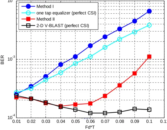
Fig. 12 BER versus normalized Doppler frequency in the two-path channel

B ... 45  Fig. 13 BER performance in the two-path channel for normalized Doppler

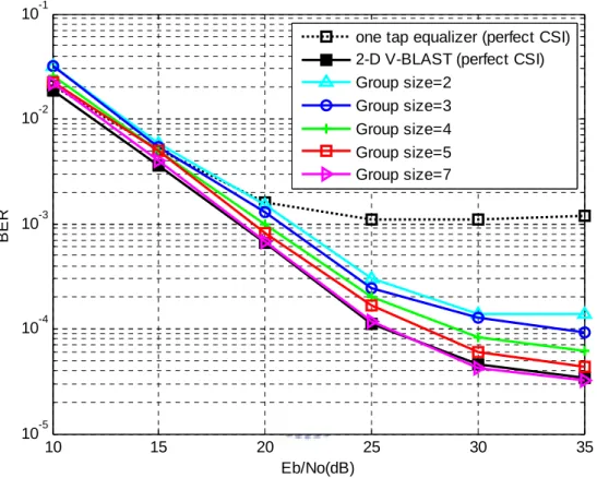
* =0.05

d T with different group size. ... 46 

Fig. 14 BER performance in the ITU Veh-B channel for normalized Doppler * =0.05

Chapter 1 Introduction

Orthogonal frequency division multiplexing (OFDM) [1] has been widely applied in wireless communication systems in recent years due to its capability of high-rate transmission and low-complexity implementation over frequency-selective fading channels. The signals received through the multipath channel suffer from severe intersymbol interference (ISI) since the delay spread becomes much larger than the symbol duration. In OFDM system, the entire channel bandwidth is divided into many narrow subchannels, which are transmitted in parallel. Therefore, the symbol duration is increased and the intersymbol interference (ISI) caused by the multipath environments is eliminated or mitigated. On the other hand, communications over multiple-input multiple-output (MIMO) channels also have been the subject of intense research over the past several years because MIMO channels can support much greater data rate and higher reliability. Spatial multiplexing is one promising technique, which can significantly increase the channel capacity by the use of multiple antennas at both the transmitter and receiver. MIMO system can be combined with OFDM system to achieve high spectral efficiency, which makes it an attractive technique for high data rate wireless applications.

The received signals in MIMO OFDM system suffer from inter-antenna interference, hence, in this paper, we solve them by using V-BLAST data detection [2] with MMSE-SIC criterion. Moreover, in high mobility environment, the relative movement between transmitter

and receiver causes Doppler spread, and the channel variations due to high mobility give a time-selectivity in one OFDM symbol so that the multipath channel is no longer time invariant. Channel time-variations in one OFDM symbol may also arise the presence of an unknown carrier frequency offset, so the orthogonal property of OFDM system is destroyed and result in the effect of inter-carrier interference (ICI) among subcarriers which degrades the performance of OFDM systems [3] [4]. This becomes more severe as mobile speed, carrier frequency or OFDM symbol duration increases.

To reduce the ICI caused by channel variations, many approaches have been proposed. In [5], the authors proposed a self-cancellation scheme which sharps the signal in frequency domain using the windowing operation in time domain to make subcarriers approximate nulls around the location of other subcarriers and, therefore, creates less ICI. In[6], it introduces a high performance equalization method by using MMSE with successive interference cancellation, but the computational complexity is very high.

[7] introduces two methods to mitigate ICI in an OFDM system with coherent channel estimation. Both methods use a piece-wise linear model to approximate channel time-variations. The first method extracts channel time-variations information from the cyclic prefix and the second method estimates these variations using both adjacent symbols. However, it acquires channel slopes by utilizing the redundancy of the cyclic prefix in the first method. While in the second method, the information of adjacent symbols has to be buffered.

In this paper, an iterative receiver architecture based on joint channel estimation and data detection is proposed to estimate the channel variations symbol by symbol, and a linear model is utilized to estimate the slope of each path without buffering information of adjacent symbols. The iterative receiver mainly consists of three-stage processing. In the initialization stage, we employ a multipath interference cancellation technique to roughly estimate multipath delays and multipath complex gains through the preamble. In the tracking stage, a

β

-tracker is applied, followed by decision-feedback (DF) DFT-based channel estimation along with V-BLAST data detection, so as to estimate the average channel variations of each path. In the final stage, we adopt a linear model to approximate time variations of each path, and a two-dimensional V-BLAST method is utilized to perform ICI cancellation and data detection.

The rest of this paper is organized as follows. In Chapter 2, we describe a MIMO OFDM system. The V-BLAST with MMSE-SIC detection algorithm is introduced briefly in Chapter 3. In Chapter 4, we present the MPIC-based decorrelation method in the initialization stage. Next, a

β

-tracker is developed in the tracking stage, and an ICI estimation is presented in the final stage. We then utilize the two dimensional V-BLAST detection to perform ICI cancellation and data detection. We present out computer simulation and performance evaluation results in Chapter 5. Finally, some conclusions are drawn in Chapter 6.

( )

⋅

* and

( )

⋅

H

x

stand for complex conjugate and Hermitian respectively. The column vector can be explicitly expressed by

x

₁

,

…

,

x

_x or

x i

_i

:

∈ … x

{

1,

,

}

, where

x

x

is the dimension of the vector . The notation

{ }

…

denotes a set, e.g. a set

x

=

{

x

₁

,

…

,

x

_x

}

x

, and the cardinality of the set is denoted by

x

. Further, the set can be expressed in a compact form

{

x i

_i

:

∈ … x

{

1,

,

}

}

.

Chapter 2 MIMO OFDM System

2.1 Transmitted Signals

SYMBOL MAPPING S/P OFDM Modulator OFDM Modulator OFDM Demodulator OFDM Demodulator Channel Estimation & Data Detection 1 Tx T N Tx 1 Rx R (1) [0] X (1)_{[ 1]} X N− ( ) [0] T N X ( ) [ 1] T N X N− N Rx (1) [ 1] R N− (1) [0] R ( ) [0] R N R ( ) [ 1] R N R N− Information Source

Fig. 1 MIMO OFDM system

Fig. 2 OFDM frame format

Fig. 1 and Fig. 2 illustrate a MIMO OFDM system and its frame format. We consider a MIMO OFDM system with transmit and receive antennas, employing subcarriers among which

T

N NR N

M subcarriers are used to transmit data symbols plus pilot tones

and the other subcarriers are used as either a DC subcarrier or virtual subcarriers at the two edges to avoid the aliasing problem at the receiver. Assume that the sets of data and pilot subcarriers indices are denoted as Q and J, respectively, where and

N−M

, ⊆ Q J Ω

{

}

= 0, ,N−1

Ω … is the set of the total subcarrier indices. The information source bits are first mapped into QPSK data symbols and are converted into N parallel data substreams through a serial to parallel (S/P) block. At the ith transmit antenna, Q QPSK data symbols X( )i

[ ]

k ,

[ ]

( )i

for k∈Q, and J pilot symbols X k , for k∈ J

N−M

( )

_[

, are modulated onto M subcarriers via

a N-point inverse Fast Fourier Transform (IFFT) unit to produce time domain samples after

insertion of zeros for DC and virtual subcarriers.

{

]

( )

_{[ ]}

}

( )

_{[ ]}

2 1 0 1 , 0 1. i i j kn N i _N k x n IFFT X k X k e n N N π − = = =

∑

≤ ≤ − ( (2.1)

[ ]

) i X where k (

represents the transmitted data point at the kth subcarrier from the ith transmit

antenna and x_ni) is the time domain sequence. A cyclic prefix (CP) is then added in front of each OFDM data symbol to eliminate intersymbol interference (ISI) caused by multipath channels as follows: ( ) ( )

_{[ ]}

: 1 i i cp = x n N− ≤ ≤ −G n N x ( (2.2) where G is the length of guard interval. And we assume that the normalized length of the

channel is always less than or equal to G in this paper to make sure that there is no ISI after removing the guard interval. As shown in Fig. 2, each OFDM frame starts with a CP-added preamble which occupies one OFDM symbol and is followed by D consecutive OFDM data

symbols. Specifically, pilot tones are alternatively inserted into the available pilot subcarriers to avoid inter-antenna interference at the receiver side, and the pilot preamble in frequency domain is denoted by Pi)

[ ]

k , for k∈Q J∪ and i=1,…,N_T.

2.2 Channel Model

In wireless communication, there may be more than one path from transmitter to receiver. Received signals come from multiple paths may be due to atmospheric reflection, refraction, or reflection from buildings and other objects. Such environment is called a multipath channel. The complex baseband representation of impulse response for a mobile wireless channel between the ith transmit antenna and the jth receive antenna can be described by

( ),

_{[ ]}

( ), 1 ( , )

_{( )}

( ), 0 , j i L j i j i j i l l l h t τ μ t δ τ τ − = ⎡ ⎤ =

∑

_⎣ − _⎦ ( (2.3) )

_{( )}

, j i l t

μ _{is the complex Gaussian fading gain of the lth path,} (j i,)

l

where τ is the excess

delay in samples of the lth path, δ

[ ]

τ is a Kronecker delta function, and L(j i,) is the number of resolvable paths. All paths μ_l( )j i,

(

t

)

, for 0≤ ≤l L( )j i, −1

( ),

_{[ ]}

( ), 1 ( , )

_{( )}

{

( ),

}

0 , exp 2 / j i L j i j i j i l l l H t k μ t j π τk N − = =

∑

− k , are assumed to be independent of each other and generated from Jakes’ model. Thus, for OFDM systems with proper cyclic extension and sample timing, the channel frequency response can be expressed as

(2.4) where is the subcarrier index.

2.3 Received Signals

We assume that both timing and carrier frequency synchronization are perfect, and that the length of channel impulse response (CIR) is always shorter than the length of the CP so as to

remove CP correctly. Let T be the sampling period, then s T T is the time

duration of one OFDM symbol after adding the guard interval.

(

)

s N G = × +

[ ]

( )j i, ( )j i,

₍

₎

l l s h n =μ t = ×n T represents the lth channel tap at time instant t= ×n Ts

(

1

)

× ≤ < + ×

corresponding to the ith transmit

antenna and the jth receive antenna. A constant channel is assumed over the time interval

s s

n T t n T t=0

(

with indicating the start of the data part of the symbol.

)

_{[ ]}

,

j i l

h n for − ≤ ≤ −G n 1 and 0≤ ≤ −n N 1 represents the lth channel tap in the guard

interval and data interval respectively. Then the received signal r( )j

( )

_{[ ]}

( ), 1 ( ),

_{[ ]}

( )

₍

₍

₎

₎

( )

_{[ ]}

1 0 , 0 1. j i T N L j j i i j l _N i l r n h n x n l z n n N − = = ⎡ ⎤ =

∑ ∑

_⎣ − _⎦+ ≤ ≤ −

( )

( )

N

at the jth receive antenna is the superposition of all distorted

transmitted signals, which can be expressed as follows:

(2.5)

[ ]

( )

where represents a cyclic shift in the base of N and z j n

2

z

represents a sample of uncorrelated additive white Gaussian noise (AWGN) with zero-mean and variance σ on the

jth receive antenna.

2.4 ICI on OFDM System

After the OFDM demodulator in Fig. 1, the received OFDM data symbols at the jth

receive antenna in frequency domain are given by

( )

_{[ ]}

{

( )

_{[ ]}

}

1 ( )

_{[ ]}

2 0 0 1 j nk N j _N n k F r n r n e k N π − ₋ = = =

∑

≤ ≤ j j T R F − ( (2.6) )

_{[ ]}

j R k

)

_{[ ]}

(i

X k

( )

which can be derived as follows:

[ ]

( ) ( )

_{[ ]}

₍

₍

₎

₎

_{[ ]}

( ) ( ) ( )

_{[ ]}

(

₍

₎

)

( ) ( ) ( )

_{[ ]}

( ) ( )

_{[ ]}

( )

_{[ ]}

, , , 2 1 1 , 0 1 0 2 2 1 1 1 , 1 0 0 0 π π π − − ₋ = − − ₋ − ₋ = = − − _{− −} = = = ⎛ ⎞ ⎡ ⎤ = ⎜_{⎜ ⎣} − _⎦+ ⎟_⎟ ⎝ ⎠ ⎛ ⎞ ⎡ ⎤ = ⎜_{⎜ ⎣} − _⎦ ⎟_⎟+ ⎝ ⎠ ⎛ ⎞ ⎜ ⎟ ⎝ ⎠

∑

∑

∑

∑

∑

j i T j i j i j nk N L j j i i j _N l _N l j nk j nk N L N j i i _N j _N l _N l n j ml j mn j nk N L N j i i _{N N N} l n l m h n x n l z n e h n x n l e z n e h n X m e e e N ( )

_{[ ]}

0 0 2 2 2 1 1 , 0 1 π π π = = = =

∑ ∑

∑ ∑

T N n i i n = N R k ( )

_{[ ]}

( ) ( ) ( )

_{[ ]}

( )

_{[ ]}

( )

₍

₎

( ) ( )

_{[ ]}

( )

_{[ ]}

, , 1 2 2 1 1 1 , 1 0 0 0 2 1 1 , 1 0 0 1 1 π π π − − − − − _{− −} = = − − ₋ = ⎛ ⎞ + ⎜ ⎟ ⎜ ⎟ ⎝ ⎠ ⎛ ⎛ ⎞ ⎞ = ⎜_⎜ ⎜_⎜ ⎟_⎟ ⎟_⎟+ ⎝ ⎠ ⎝ ⎠ ⎛ ⎞ = ⎜_⎜ − ⎟_⎟+ ⎝ ⎠

∑

∑

∑

j i j i j j n k m j ml N L N j i _{N N} i j l l n j ml N L j i _N i j l l 1 = = = =

∑ ∑

∑ ∑

∑ ∑

T T T i m i m = N i N N Z k h n e e X m Z k N F k m e X m Z k N ( )

_[

_]

( )

_{[ ]}

( )

_{[ ]}

( ) ( ) ( ) ( )

_{[ ]}

( )

_{[ ]}

, 1 , , , j j i i j N j i i j i i j H k m X m Z k H k m Z k − = + ⎛ ⎞ ⎜ ⎟ + ⎜ ⎟ ⎜ ⎟ ⎜ ⎟ ⎝ ⎠ ( (2.7) (2.8) ( )

_{[ ]}

R k k∈Q

[ ]

[ ]

[

]

1 0, , , i m m k ICI k X k H k m X = = ≠ =

∑

+

∑

1 1 0 N i m − = =

∑∑

T T N N ∪ J j)

[ ]

( )

[ ]

Z k denotes the FFTof for , where z j n (

and the second term on the right hand side of (2.8) represents ICI due to the Doppler spread caused by high mobility and cannot be neglected as the maximum Doppler frequency increases. Define F_l j i,)

( )

k

( )

_{( )}

( )

_{[ ]}

as the DFT of the lth channel tap with respect to time-variation:

2 1 , , 0 0 & 0 1 j nk N j i j i _N l l n F k h n e l G k N π − ₋ = =

∑

≤ ≤ ≤ ≤ − (2.9) ( Then H j i,)

[

]

( ) , k

[

]

m which denotes the channel frequency response from the mth subcarrier on

the kth one can be defined as

( ) ( )

₍

₎

( ) , j i ( )

_{[ ]}

2 ( ) 2 , 2 1 1 1 , , , 0 n 0 0 1 j n k m j ml 1 j i j ml L N L j i _{N N} j i _N l l l l h n e e F k m e N N π − π π − − _{− −} − ₋ = = = ⎡ ⎤ = _{⎢ ⎥} = − ⎣ ⎦

∑

∑

∑

, j i H k m (2.10) Furthermore,

( ),

_{[ ]}

( ), 1 ( ), 2 ,0 0 , j i _{j kl} L j i j i _N l l H k k e π μ − ₋ = =

∑

( ) (2.11) ( )

_{[ ]}

1 , , ,0 0 1 where μ − = =

∑

N j i j i l l n h n N 0

is the average of the lth channel tap over the time duration of

[ ]

s

t N T

≤ ≤ × . Therefore, H(j i,) k k,

[

represents the DFT of this average.

As the channel is time-invariant or we assume that the channel is quasi-static within one

OFDM data symbol, h nl

]

l

( )

_{[ ]}

( ),

_{[ ]}

( )

_{[ ]}

( )

_{[ ]}

1 , T N j j i i j i

becomes a fixed complex fading gain ( h ). Then, because of the orthogonal property of the subcarriers, the second term of (2.8) becomes 0, which means no ICI, and (2.8) can be easily reduced as follows:

k H k k X k Z k = =

∑

+ ( )j

_{[ ]}

( )j i, ( )i ( )j p (2.12) R

And the received pilot preamble at the jth receive antenna can be described by

[ ]

,

[ ]

[ ]

1 T N i R k H =

∑

k = k P k∈ ∪Q J k +Z k (2.13) for .

Chapter 3 V-BLAST

 

Detection

   

In this chapter, the conventional V-BLAST detection method with MMSE-SIC algorithm is introduced to perform data detection in MIMO OFDM system. We first consider a MIMO system with transmit and receive antennas, which can achieve high data rates by transmitting simultaneously different data on the different transmit antennas, and

T

N NR

T R

N ≤N . A single data stream is split into substreams, each of which is transmitted using one of the transmit antennas. The transmit diversity introduces spatial interference. The signals transmitted from various antennas propagate over independently scattered paths and interfere with each other upon reception at the receiver. After passing through the channel (assuming quasi-stationary), each receive antenna receives the signals radiated from all transmit antennas. Let T N T N T N 1, 2, , T T N X X X ⎡ ⎤ = ⎣ ⎦ X R = HX + Z R NR NR H N_R×N_T H_{j i,} i

denote the vector of transmit symbols, then the corresponding received signal vector can be written as

(3.1) where is an -component column vector of the received signals across the receive antenna, is a matrix with representing the channel frequency response between transmit antenna and receive antenna j , and is the AWGN noise vector with zero mean and variance

Z 2

σ .

In the MMSE detection algorithm with successive interference cancellation (MMSE-SIC) [8], the expected value of the mean square error between transmitted signal X and a linear

combination of the received vector w RH is minimized as follows

(

)

{

2

}

min E X w R− H w NR×NT (3.2) where is an matrix of linear combination coefficients given by

(

)

1 2 T H H H N σ − = + w H H I H T T N ×N (3.3) T N

I is an identity matrix. Using H i w i H i i Y = w R

, the decision statistics for the symbol sent from antenna is obtained as

(3.4)

H H

i

w is the ith row of

where w N_R

i ˆ_i

consisting of components. The estimate of the symbol sent from antenna , denoted by X , is obtained by making a hard decision on Y_i

( )

ˆ i i X =Q Y X X (3.5) In an algorithm with interference suppression only, the detector calculates the hard decisions

estimates by using (3.4) and(3.5) for all transmit antennas.

In a combined interference suppression and interference cancellation algorithm, the interference contribution from already-detected components of is subtracted from the received signal vector, resulting in a modified received vector in which fewer interferers are present. As mentioned in [2], when interference cancellation is used, the order in which the components of are detected becomes important to the overall performance of the system. Let the ordered set S ≡

{

k k1, 2, ,kN_T

}

be a permutation of the integers 1

specifying the order in which components of the transmitted symbol vector are extracted. , 2, ,N_T

The optimal detection order is determined to maximize the minimum post-detection SNR of all data streams. A result is that simply choosing the best post-detection SNR at each stage in the detection process leads to the globally optimum ordering, S_opt.

(

i 1

)

The receiver starts from first iteration = whose detection order is and computes its signal estimate by using (3.4)and(3.5). The received signal in this iteration is denoted by . For calculation of the next iteration

1

k

R

1

R

(

i=2

)

, the interference contribution of the hard estimate

1

ˆ

k

X is subtracted from the received signal and this modified received signal denoted by is used in computing the decision statistics for iteration 2 from (3.4) and its hard estimate in Eq. (3.5). This process continues for all other iterations.

1 R

2 R

i ˆk_i

After detection of iteration i whose detection order is k , the hard estimate X is

subtracted from the received signal to remove its interference contribution, resulting in modified received signal :

i R 1 i+ R

( )

1 ˆ i _i i+ = i−Xk k R R H

( )

i k H _i H (3.6)

(

where denotes the k th column of . The operation ˆ

)

i _i k k X H ˆ i k in (3.6) replicates the interference contribution caused by X in the received vector. is the received vector which is free from interference coming from

1 i+ R 1 2 ˆ _, ˆ _{, ,} ˆ i k k k X X X 1 i+ R R

. For estimation of the nest stage, this signal is used in (3.4) instead of . Finally, a deflated version of the channel matrix is calculated, denoted by

i k

H , by zeroing column k k₁, ₂, ,k_i of H . The deflation is needed as the interference associated with the current symbol has been estimated

and cancelled.

The full V-BLAST with MMSE-SIC detection algorithm is described as a recursive procedure, including determination of the optimal ordering, as follows:

(

)

( )

( )

( )

( )

1 1 2 1 2 1 1 1 Initialization : arg min R sion : ˆ ˆ T i i i i i i i H ecur H H N j j k i k H k k i i k i i k k k Y X Q Y X σ − + = = + = = = = = − R R G H H I H G w G w R R R H

(

)

{1 }

(

)

1 2 2 1 arg min_, 1 1 i T i k H H H i N i _{j k k} i j i i σ − + _∉ + = = + = = + H H G H H I H G

( )

Gi j k

where is the jth column of G_i, and v is the Euclidean norm of the vector v.

i

k X

Since the post-detection SNR for the th detected component of is

2 2 i i k k X SNR σ = w

( )

2 i k , 2 1 g mi j 1 ar n k = G X k_i

(

NT i 1

)

j corresponds to the strongest detected component of . Similarly,

corresponds to the strongest detected component among the remaining − +

opt

components. Thus, it determines the elements of S , the optimal ordering.

The V-BLAST architecture is essentially a single carrier signal processing algorithm. Therefore, to combine it with OFDM, the V-BLAST detection process has to be performed on

every subcarrier at the receiver to achieve high data rate transmission in frequency selective fading channels. As OFDM effectively divides the frequency selective channel into a number of flat fading subchannels, the MIMO OFDM system comprises a number of narrow band MIMO systems on different subcarriers. As the same detection algorithm is used on each subcarrier, MIMO OFDM system is basically a per-subcarrier MIMO structure, which performs V-BLAST detection on each subcarrier.

Chapter 4 Iterative Receiver

 

The iterative receiver based on joint channel estimation and data detection mainly consists of three-stage processing. In this section, we first present the MPIC-based decorrelation method for the initialization stage. In the following tracking stage, we adopt a

β

-tracker followed by DF-DFT based channel estimation method to estimate the frequency response of average channel variations of each path. With the estimated channel frequency response, the detection of transmitted signals can be performed by applying V-BLAST with MMSE-SIC algorithm described in chapter 3. In the final stage, we approximate channel variations of each path with a linear model. Then, a two-dimensional V-BLAST method is utilized to perform ICI cancellation and data detection. The block diagram of the channel estimation in the tracking stage and the ICI cancellation in the final stage is shown in Fig. 3.

β ( ) [ ] j R k ( , ) 1 [ , ] j i H k k ( ) [ ] i X k ∧ ( , )j i_{[ , ]} H k m ( , ) [ , ] j i v H k k ( , ) [ , ] j i H k m ( ) [ ] i X k ∧

Fig. 3 Block diagram of the channel estimation in the tracking stage and the ICI cancellation in the final stage.

4.1 Initialization Stage: The MPIC-Based Decorrelation Method

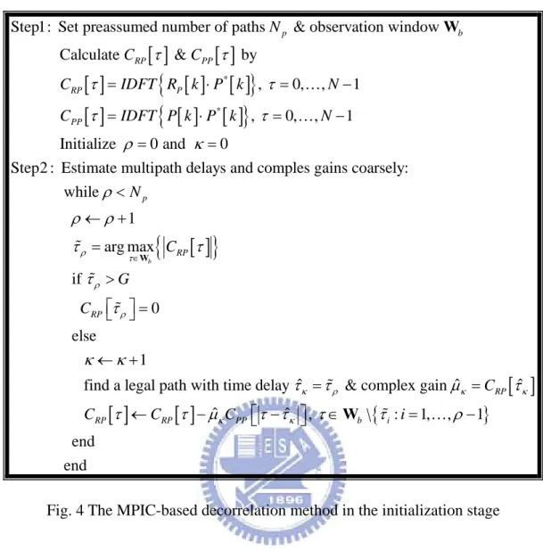
In this stage, we roughly estimate multipath delays and multipath complex gains through the preamble placed at the beginning of each OFDM frame. We all know that CIR can be estimated by using the preamble placed at the beginning of each OFDM frame, while the difficulty is that for most wireless standards, the preamble does not have ideal auto-correlation due to the use of either guard band or non-equally spaced pilot tones. Fig. 4 outlines the MPIC-based decorrelation method to estimate CIR path-by-path by canceling out already known multipath interference. Since the preambles transmitted from different antennas do not interfere with each other at the receiver side, channel estimation can be independently performed for each transceiver antenna pair, and therefore the antenna indices j and i are omitted in the following. In step 1, we first define two parameters and which represent a multipath observation window and a presumed number of paths in a mobile radio channel, respectively. Next, we calculate the cyclic cross-correlation

b

W N_p

[ ]

RP

C τ between

the received and the transmitted preamble by

{

[ ]

[ ] [ ]

*

}

, 0 RP P C τ =IDFT R k ⋅P k τ = …, ,N−1 (4.1)

[ ]

PP C

The normalized cyclic auto-correlation τ of the transmitted preamble can also be calculated by

{

[ ]

[ ] [ ]

*

}

, 0, , 1 PP C τ =IDFT P k ⋅P k τ = … N− (4.2)

ρ and κ, which stand for a path counting variable and the number of legal paths Both

found by the MPIC-based decorrelation method, respectively, are initialized to zero. In step 2, we start by increasing the value of the path counting variable ρ by one, and picking only one path whose time delay τρ yields the largest value in CRP

[ ]

τ , for τ∈ W . If the time b

delay τ_ρ

0

RP

C ⎡ ⎤ =_{⎣ ⎦}τ_ρ

κ th

is larger than the length of the CP, this path is treated as an illegal path, and we discard it by setting . Otherwise, we increase the number of legal paths found,

, by one, and then reserve this path as the κ legal path with time delay τˆ_κ =τ_ρ

[

and complex path gain μˆ_κ =C_RP τˆ_κ

]

. The replica of the interference associated with this legal path is regenerated and subtracted from CRP

[ ]

τ to obtain a refined cross-correlation

function:

[ ]

[ ]

ˆ ˆ , \

{

: 1, , 1

}

RP RP PP b i

C τ ←C τ −μ_κC _⎣⎡τ τ− _κ ⎤_⎦ τ∈W τ i= … ρ− (4.3) where“←” is the assignment operation. We continue the iterative process of the step 2 until

[ ]

[ ]

[ ]

{

[ ] [ ]

}

[ ]

{

[ ] [ ]

}

* *

Step1: Set preassumed number of paths & observation window Calculate & by , 0, , 1 , 0, , 1 Initialize p b RP PP RP P PP N C C C IDFT R k P k N C IDFT P k P k N τ τ τ τ τ τ ρ = ⋅ = − = ⋅ = − W … …

[ ]

{

}

0 and 0

Step2 : Estimate multipath delays and comples gains coarsely: while 1 arg max if 0 b p RP RP N C G C ρ _τ ρ ρ κ ρ ρ ρ τ τ τ τ ∈ = = < ← + = > ⎡ ⎤ = ⎣ ⎦ W

[ ]

[ ]

[ ]

{

}

else 1 ˆ ˆ ˆ

find a legal path with time delay & complex gain

ˆ ˆ , \ : 1, , 1 RP RP RP PP b i C C C C i κ ρ κ κ κ κ κ κ τ τ μ τ τ τ μ τ τ τ τ ρ ← + = = ⎡ ⎤ ← − _⎣ − _⎦ ∈W = … − end end

Fig. 4 The MPIC-based decorrelation method in the initialization stage

4.2 Tracking Stage:

β

-tracker

Through the initialization stage, we are able to obtain information on the number of paths

( )j i,

(

)

p

N

κ ≤ , the multipath delays τˆ_l( )j i, , and the multipath complex gains μˆ_l( )j i, , for

( )

{

,

}

1, , j i

l∈ … κ . Without loss of generality, we assume that the multipath delays do not vary over the duration of each OFDM frame. In this stage, we also suppose that the channel is quasi-static within one OFDM data symbol, which means the multipath complex gains of channel model are unchanged, so as to estimate the average channel variations of each path.

[ ]

( )

Accordingly, the corresponding channel estimator Hˆ j i, k k,

(

for the frequency response

[ ]

( )

) j i,

, ,

j i

H k k can be formed by a summation of κ exponential functions as follows:

( ),

_{[ ]}

( ), 1 ( ),

{

( ),

}

0 ˆ _{, ˆ exp 2 ˆ} j i j i j i j i l l l H k k j k N κ μ π τ − = =

∑

− (4.4)

In this stage, a

β

-tracker followed by DF DFT-based channel estimation is applied to track channel. We start by utilizing the decision feedback (DF) DFT- based channel estimation method, using the ML criterion [9] [10][11][12], which is provided in the following:

( ) ( )

(

( ) ( )

)

1 ( )

( )

( ) 1 ( ) , , , , , , , , , ˆ j i j i j i j i j i ˆ i j i v DFT d IDFT d DFT d IDFT v − − = H F F F F X R ( ) ( ) (4.5)

[ ]

{

}

, , ˆ j i ˆ j i _{, : = 0, , 1} v Hv k k k N

where v is the iteration number from 1 to V , H = ∈Ω … −

( ) ( ) ( )

is the estimated channel frequency response between the ith transmit antenna and the jth receive antenna at the vth iteration, ˆ

{

ˆ [ 1],..., ˆ [ ]

}

i i i

diag X X

= Θ Θ_Θ

X

Θ Q

consists of the decision data symbols in which is a subset of used to track channel variations and Xˆ [( )i k can be ] obtained by applying the previously estimated channel frequency response to the V-BLAST data detection with respect to the received signals. F_{d DFT}( )_,j i, represents the Θ×κ( )j i,

( )

truncated DFT matrix whose ( m,l )th entry is defined as exp

{

−j2π τΘm lj i, /N

}

, ( ) , , j i d IDFT F ( is the κ j i,)× Θ ( ),

(

( ),

)

, ,

truncated IDFT matrix which can be equivalently expressed as

H

j i j i

d IDFT = d DFT

F F , and F_DFT(j i,) is the N×κ( )j i, truncated DFT matrix. For simplification, the subscripts “DFT” and “IDFT” are omitted, then F_{d DFT}( )_,j i, , F_{d IDFT}( )_,j i, and F_DFT(j i,)

( are replaced by ) , j i d F

( )

( ), , H j i d

F , and F(j ,i) respectively. We assume that the data interference signals from other transmit antennas can be reconstructed and cancelled perfectly from the received signals

( )

,

( )j

R . Thus, the refined signals corresponding to the j i

( ) ( )

_{[ ]}

( )

_{[ ]}

( )

_{[ ]}

( )

_{[ ]}

( )

_{[ ]}

th antenna pair can be represented as

[ ]

( )

_{[ ]}

, , _ˆ , _ˆ , j i j i j j m m j i v = Rv k =R k − H k k X k =H k k∈ R , Θ , k, X i m i≠

∑

k +Z k (4.6) Moreover, since the refined signals from different antenna pair do not interfere with each other, we can perform the channel estimation for each transceiver antenna pair and, for simplification, the superscript “

( )

j, i ＂ and “

( )

i ＂are dropped hereafter. Therefore, the

DF-DFT based channel estimation method can be expressed as follows:

(

)

1 ˆ H ˆ v d d v − F F H 1R d − F X = H F (4.7)

This is, however, not a good solution in fast time-varying channels because decision data symbols easily induce the error propagation effect. Therefore, pilot tones play an important role in fast fading channels. While in the slowly fading channels, decision data symbols are more reliable than pilot tones due to the number of data subcarriers are much more than pilot tones. Hence, we can modify the first iteration by adopting pilot tone as well as decision data symbols simultaneously to perform channel estimation at the first iteration. This, we modify the first iteration with v=1 by the

β

-tracker in which the current channel can be weighted with the channel estimated over data symbols in the previous time slot and the channel estimated over pilot signals in the current time slot due to that the current channel is related to the previous channel, which depends on how fast the channel varies. Therefore, The

β

-tracker for the first iteration (v=1) can be described as follows:

(

)

1 ˆ ₁ ˆ ˆ v = −β v− +β p H H H 0 ˆ H

(

)

1 ₁ ˆ H H p p p p p p − ₋ = H F F F F X R p X R_p p F

(4.8)

where represents the channel estimated over data symbols in previous time slot, denotes the channel estimated by DF DFT-based channel estimation over pilot subcarriers in which is the diagonal matrix of pilots, is the corresponding received pilot signals, and is the J×κ( )j ,i truncated DFT matrix over pilot subcarriers. Likewise, since the received pilot signals from different antenna pair do not interfere with each other, we can also perform the channel estimation o for each transceiver antenna pair. In order to initialize the channel estimator of (4.8), the CSI estimated in the last iteration of previous time slot has to be taken as the initial value of the CSI for the current time slot.

Then, we can construct an MMSE cost function over all subcarrier indices, and derive the minimum β as follows:

(

) (

)

( )

2 * * * * * ˆ argmin ˆ ˆ argmi ˆ ˆ ˆ ˆ argmi argmin v v v v v v v v v v v v v v E f β β β β β β ⎡ ⎤ = _⎢ − _⎥ ⎣ ⎦ ⎡ ⎤ = _⎢ − − _⎥ ⎣ ⎦ n n E E ⎡ ⎤ = _⎣ − − + _⎦ = H H H H H H H H H H H H H H v H

( )

f (4.9)

where is the true value of current channel frequency response. Each component of β can be derived separately in the following. From (4.8) and (4.9), we have

(

)

(

)

(

(

)

)

(

)

(

)

(

)

* * * 1 1 2 _{* 2 *} 1 1 1 ˆ ˆ ₁ ˆ ˆ ₁ ˆ ˆ ˆ ˆ ˆ ˆ ˆ ˆ 1 1 1 v v v p v p v v p p v p p E E E β β β β β β β β β β − − − − − ⎡ ⎤ ⎡ ⎤ = − + − + ⎣ ⎦ ⎣ ⎦ ⎡ ⎤ = _⎣ − + − + − + _⎦ H H H H H H H H* * H H H H 1 ˆ ˆ v− H H (4.10) Let the estimation of be the summation of the true previous value plus a noise term, and the estimation of

1

v−

H

P

H also be the summation of the true current value plus a noise term as follows: (4.11) 1 1 ˆ ˆ v v v p v v − = − + = + H H Z H H Z

(

)

(

)

1 −

(

(

)

{

}

with

(

)

)

)

(

)

}

(

) (

(

)

{

{

}

1 2 * 1 1 2 2 0 2 v v v H H H d d d v 1 ₁ 1 ₁ 1 1 1 here H H d d d v 1 1 1 1 1 1 1 H 1 1 1 1 , w H H D v D D v H H D v v H D D D − − − − − − − − ⎡ ⎢⎣ Z W X Z W X Z W X Z Z X W W W W W

{

H

}

D v H D v H D − − − − ⎡ ⎤ ⎢ ⎥ ⎣ ⎦ ⎡ ⎤ ⎣ ⎦ F F Z D d d d − ₋ − ₋ − − − ⎡ ⎤ ⎢ ⎥ ⎣ ⎦ = = ⎤ ⎥⎦ F F X Z W F F F F z s b E E E Tr E Tr E Tr N Tr E σ σ σ − = ⎣⎡ − − ⎤⎦ = = = = = Z Z Z F F F F X Z W X W X (4.12) and

(

)

(

)

(

(

)

)

{

}

(

) (

)

(

)

(

)(

)

{

}

{

}

2 * 1 ₁ 1 ₁ 1 2 2

2 , where is pilot powe

v v v H H H H H p p p p v p p p p v 1 1 1 1 1 , where H H H P p v P p v P p p p H E Tr E − − − − − ⎡ ⎤ = _{⎢ ⎥} = ⎣ ⎦ ⎡ ⎤ = W X Z W X Z W F F F F W X ZP p v W X ZP p v H H H P p v v p P H z P P p p E E Tr E Tr σ σ _σ σ − ₋ − ₋ − − ⎡ ⎤ = ⎣ ⎦ ⎡ ⎤ = ⎢_⎣ ⎥_⎦ ⎢ ⎥ ⎣ ⎦ ⎡ ⎤ = _{⎣ ⎦} = Z Z Z F F F F X Z F F F F X Z W X Z Z X W W W r

{

(4.13)

}

Tr ⋅

(

)

1 1 * * * * 2 * * * * 2 1 1 1 1 1 1 * * * * 2 1 1 1 0 * * * * 1 1 1 2 v v v v v v v v v v h v v v v v v h v v v v v v h d v v v v v v E E E E E E E E E J f T E E E σ σ σ π − − − − − − − − − − − − − − = = ⎡ ⎤= ⎡ ⎤= ⎡ ⎤= ⎣ ⎦ ⎣ ⎦ ⎣ ⎦ ⎡ ⎤= ⎡ ⎤= ⎡ ⎤= ⎣ ⎦ ⎣ ⎦ ⎣ ⎦ ⎡ ⎤= ⎡ ⎤= ⎡ ⎤= ⎣ ⎦ ⎣ ⎦ ⎣ ⎦ ⎡ ⎤= ⎡ ⎤= ⎡ ⎤= ⎣ ⎦ ⎣ ⎦ ⎣ ⎦ H Fh H Fh H H h F Fh h h H H h F Fh h h H H h F Fh h h H H h F Fh h h 2

(

)

0 2 hJ f Td σ π

( )

0 J ⋅ d

denotes the trace of a square matrix. where

Furthermore, the autocorrelation function of the channel frequency response is as follows:

(4.14)

where denotes the zero-order Bessel function of the first kind, and f is Doppler frequency in hertz, σ_h2 is the channel power, and is the time duration of one OFDM symbol after adding the guard interval.

T

(

)

(

)

(

)

(

)

(

)

(

)

(

)

(

)

(

)

(

)

(

)

(

)

1 2 * * * * 1 1 1 1 1 * 2 * * 1 2 _{2 2 2} 0 2 2 2 2 0 ˆ ˆ _{1 1} 1 1 1 2 1 2 v v v v v v v v v v v v v v v v h h d h d h E E E E E E E J f T J f T β β β β β β β σ σ β βσ π β β σ π β σ σ − − − − − − − ⎡ ⎤ ⎡ ⎤

Hence, from (4.12) ~(4.14) , (4.10) is equivalent to

⎡ ⎤ ⎡ ⎤ = − _{⎣ ⎦}+ _{⎣ ⎦} + − _{⎣ ⎦} ⎣ ⎦ ⎡ ⎤ ⎡ ⎤ ⎡ ⎤ + − _{⎣ ⎦}+ _{⎣ ⎦}+ _{⎣ ⎦} = − + + − + − + + Z Z H H H H Z Z H H H H H H Z Z (4.15)

(4.16)

(

)

(

)

(

)

(

)

(

)

* * * 1 * * 1 2 2 0 ˆ ₁ ˆ ˆ 1 1 1 2 v v v p v p v v v v v h d h E E E E E J f T β β β β β σ π βσ − − ⎡ ⎤ ⎡ ⎤ = − + ⎣ ⎦ ⎣ ⎦ ⎤ = − _⎦ ⎡ ⎤ ⎡ ⎤ = − _{⎣ ⎦}+ _{⎣ ⎦} = − + H H H H H H H H H H

(

)

(

)

(

)

(

)

(

)

(

* * 1 * * 1 * * 1 2 2 0 ˆ ₁ ˆ ˆ ˆ ˆ 1 2 v v p v v v p v v v h d h E E J f β β β σ π βσ − − − ⎡ ⎤ = _⎣ − + _⎦ ⎡ ⎤ ⎡ ⎤ ⎣ ⎦ ⎣ ⎦ ⎡ ⎤ ⎡ ⎤ ⎣ ⎦ ⎣ H H H H H H H H H H H

( )

(

)

(

)

(

)

(

)

(

)

(

)

(

)

(

)

(

)

(

)

(

)

(

)

(

)

(

(

)

)

1 1 1 2 _{2 2 2 2 2 2 2} 0 0 2 2 2 2 2 0 0 2 2 2 2 2 2 2 2 0 0 2 argmin argmin 1 1 2 1 2 1 2 1 2 argmin 2 2 2 4 2 4 2 2 v v v v v h h d h d h h d h h d h h h h d h h d h f J f T J f T J f T J f T J f T J f T β β β β β β σ σ β βσ π β β σ π β σ σ β σ π βσ β σ π βσ σ σ σ σ π σ β σ σ σ π β σ σ − − − = ⎡ = _⎣ − + + − + − + + ⎤ − − − − − − + _⎦ ⎡ = _⎣ + − + + − − + + + Z Z Z Z Z

(

)

(

1

)

2 2 0 2 2 v− σhJ π f Td ⎤ − _⎦ Z

( )

(

)

* * 1 ˆ ˆ v v E β ⎡_⎣H H₋ ⎤_⎦+β ⎡_⎣H (4.17)

)

E E T β β β β + + + 1 1 v v E⎡_⎣ ⎤_⎦ E = − = − = − H H v⎦

Therefore, apply (4.15)~(4.17) into (4.9) then we can get the following equation:

(4.18)

By taking f β 0

β

∂

, the optimum value of β is given by

= ∂

(

)

(

)

1 1 0 2 2 2 2 0 2 2 2 2 2 2 v v v h h d h h d J f T J f T σ σ σ π β 2 2 2 σ σ − σ π σ − + − = + − + Z Z Z (4.19) We can observe from the above equation that as the mobile speed is slow,

and then

(

)

0 2 d 1 J π f T 1 1 2 2 2 v v v σ β J₀

(

2π f T_d

)

0 and 1 σ −σ − + Z Z Z

; as the mobile speed is fast, β

v V

.

It is noted that, after the first iteration, we execute the channel tracking process of (4.7) for the second and subsequent iterations until a stopping criterion holds. The stopping criterion is to check whether the iteration number reaches the maximum value of . The channel

tracking process for the current time slot will be stopped when the above condition holds.

β

Fig.4 outlines the -tracker followed by DF DFT-based channel estimation method to estimate the average channel variations in the tracking stage. We perform the channel estimator described above for each transceiver antenna pair respectively, and then after each iteration we have Hˆ( )j i, = ˆ( )j i,

[ ]

k∈Ω= 0,

{

…,N−1

}

i= …1, ,NT 1, , _R , : v Hv k k for and

[ ]

( ), ˆ j i _, v H k k for i 1, ,N_T

j= … N . With the knowledge of = … and j= …1, ,N_R

( )

(

)

(

)

(

)

1 1 ₁ For 1

For each antenna pair , where 1 ,1 If 1 ˆ ˆ ˆ 1 ˆ where else ˆ R T v v p H H p p p p p p H v d d v V j i j N i N v β ₋ β − ₋ ≤ ≤ ≤ ≤ ≤ ≤ = = − + = = H H H H F F F F X R H F F F ( ) ( )

_{[ ]}

( )

_{[ ]}

( )

_{[ ]}

( )

_{[ ]}

, we can detect data by performing V-BLAST with MMSE-SIC algorithm on each subcarrier as mentioned in chapter 3. ( ) ( )

_{[ ]}

_{

_}

1 ₁ , , , , , ˆ ˆ ˆ where , , End End ˆ ˆ We can get , : = 0, , 1

Detect data using V-BLAST with MMSE-SIC algorithm: H d v j i j i j j m m v v m i j i j i v v R k R k H k k X k k H k k k N − ₋ ≠ = = − ∈ = ∈ −

∑

F X R R Θ H Ω … 0 ˆ Assign 1 End ˆ ˆ Assign _V v= +v = X H H

β

-tracker followed by DF DFT-based channel estimation method in the tracking stage Fig. 5

4.3 ICI Estimation

In the presence of Doppler caused by high mobility, due to the ICI term of (2.8), using the estimate of average channel for data detection results in poor performance. This motivates the need to perform ICI estimation.

In this stage, we adopt a linear model with a constant slope over the time duration of one OFDM symbol to approximate time variations of each path.When the linear model is applied, we will derive the frequency domain relationship, similar to (2.8). We first consider the SISO case with one transmit and one receive antenna by omitting the superscript “

( )

j i,

)

i

[ ]

[ ] [

] [ ]

[ ] [ ]

[ ] [

] [ ]

1 0 1 0, ICI , , , N m N m m k Y k X m H k m Z k ＂ and “

(

＂, and in the end of this section we will apply it to MIMO case.

The received signal of SISO case is as follows:

X k H k k X m H k m Z k − = − = ≠ = + = + +

∑

∑

(4.20)

[ ]

X k is transmitted symbols which we assume it is known, and H k m

[

,

]

where denotes

the channel frequency response from the mth subcarrier on the kth one which can be expressed as:

[

]

1 1

[ ]

2 ( ) 2 0 n 0 1 , l j m j n k m L N N N l l H k m h n e e N π τ π − − − _{− −} = = ⎡ ⎤ = _{⎢ ⎥} ⎣ ⎦

∑ ∑

. (4.21)

[ ]

,

H k k is known which can be obtained from

Furthermore, we assume

β

-tracker and can

[ ]

1 ,0 2 0 , l j k L N l l H k k e π τ μ − ₋ = =

∑

(4.22)

where μ_l,0 is the average channel variation of the lth path. Through an IDFT, we have

[ ]

2 1 ,0 0 , 0 1 l j k N N l k H k k e l L π τ μ − = =

∑

≤ ≤ − . (4.23)

Let μ_l,1 denote the slope of the th path in the current OFDM symbol. To perform the linearization, knowledge of the channel at one time instant in the symbol is necessary. As mentioned in [7], let

l

[ ]

E z represent the average of . Then for the th channel tap, z l

[ ]

2 ,0 l l E⎡_⎢⎣μ −h n ⎤_⎥⎦ is minimized for 1 2 N n=_⎜⎛ − ⎞_⎟ ⎝ ⎠. Therefore, we approximate l 2 1 N h ⎡_⎢ − ⎤_⎥ ⎣ ⎦ ,0 l

with μ . We will have

,0 ˆ ₁ 2 l l N h ⎡_⎢ − =⎤_⎥ μ ⎣ ⎦ . (4.24)

Consider linearization around 1 2 l N h ⎡_⎢ − ⎤_⎥. Then,

[ ]

⎣ ⎦ h nl

[ ]

can be approximated as follows:

,1 1 ,0 0 1 2 l l l N h n =μ ⎛_⎜n− + +⎞_⎟ μ ≤ ≤ −n N ⎝ ⎠

[

]

(4.25) Inserting (4.25) into (4.21), we will have

2 2 ( ) ,1 ,0 0 , 1 0 , 1 l j m j n k m L N N N l l l N H k m n e e k m N N π τ π μ μ − − − _{− −} = = ⎧ ⎡ ⎛ ⎞ ⎤ ⎫ =

∑ ∑

1_⎨ 1_{⎢ ⎜} − + +_{⎟ ⎥ ⎬} ≤ ≤ − 0 n 1 2 ⎝ ⎠ ⎣ ⎦ ⎩ ⎭ (4.26)

[ ]

Y k R

[ ]

Subtract the non- ICI term from the received signals and we will have k

[ ]

[ ] [ ]

1

[

0, N m m as follows:

[ ]

,

[ ] [

]

k

]

, R k Y k X k H k k Z − = ≠ = − =

∑

+ ,1 l X m H k m k (4.27)

Then we can construct an ML cost function and the slope of each path μ can be found by minimizing the following cost function: