適用於畫面間小波轉換視訊編碼之改良式移動補償時間濾波技術

全文

(1)國立交通大學電子工程學系電子研究所碩士班碩士論文. 適用於畫面間小波轉換視訊編碼之改良式移動補償時間濾波技術 Enhanced Motion Compensated Temporal Filtering for Interframe Wavelet Video Coding. 研究生：蔡家揚指導教授：杭學鳴博士中華民國九十四年六月.

(2) 適用於畫面間小波轉換視訊編碼之改良式移動補償時間濾波技術 Enhanced Motion Compensated Temporal Filtering for Interframe Wavelet Video Coding. 研究生：蔡家揚指導教授：杭學鳴博士. Student: Chia-Yang Tsai Advisor: Dr. Hsueh-Ming Hang. 國立交通大學電子工程學系電子研究所碩士班碩士論文. A Thesis Submitted to Department of Electronics Engineering & Institute of Electronics College of Electrical Engineering and Computer Science National Chiao Tung University in Partial Fulfillment of Requirements for the Degree of Master of Science in Electronics Engineering July 2005 Hsinchu, Taiwan, Republic of China. 中華民國九十四年六月. ii.

(3)

(4)

(5)

(6)

(7) 適用於畫面間小波轉換視訊編碼之改良式移動補償時間濾波技術. 研究生：蔡家揚. 指導教授：杭學鳴. 國立交通大學電子工程學系電子研究所碩士班. 摘要在本項研究中，我們將改良式移動補償時間濾波技術(motion compensated temporal filtering) 整合進畫面間小波轉換視訊編碼 (interframe wavelet video coding)之架構中。畫面間小波轉換視訊編碼可同時提供畫質、時間解析、與空間解析之可調性。此外，在高位元率時，它具有與 H.264/AVC 可相比較之編碼效率。在本論文中，我們針對在移動補償時間濾波與移動資訊可調性技術進行探討。移動補償時間濾波是一個在決定編碼的表現非常重要的要素。我們修改源自於 H.264/AVC 之移動估測方法與其編碼方式，並將其運用至畫面間小波轉換視訊編碼架構中。並且，我們也將框內方塊(I-block)、雙方向移動估測(Bi-directional motion estimation)、及移動成本函式調整等技術運用至其中。此外，我們針對以 h.264/AVC 為基礎之畫面間小波轉換視訊編碼提出移動資訊切割技術(motion information partitioning)。藉由針對移動向量進行不同精確度與搜尋方塊大小的編碼，我們可以將移動相量切割為多層次(multi-layer)。根據可調性的要求，如空間解析、位元率或複雜度考量等，可決定解碼所需之層次數目。由實驗結果可發現其在主觀視覺感受的改良.

(8) Enhanced Motion Compensated Temporal Filtering for Interframe Wavelet Video Coding Student: Chia-Yang Tsai. Advisor: Dr. Hsueh-Ming Hang. Department of Electronics Engineering & Institute of Electronics National Chiao Tung University. Abstract An enhanced motion compensated temporal filtering (MCTF) coding scheme is incorporated into the interframe wavelet coding architecture in this study. Interframe wavelet video coding can provide SNR, temporal, and spatial scalability simultaneously. Furthermore, it has a comparable coding performance to H.264/AVC at high bit rates. In this thesis, we propose improvements on MCTF and motion information scalability. Motion compensated temporal filtering (MCTF) is an essential component in deciding the coding performance of an interframe wavelet system. We modify the motion estimation syntax/scheme originally specified in the H.264/AVC and fit it into the interframe wavelet structure. In addition, the techniques of I-block, bi-directional motion estimation, and motion cost function adjustment are employed to improve image quality. Furthermore, in the original interframe wavelet video coding, the motion information is non-scalable and it may become the dominate portion of the entire bitstream at low bit rates. We propose a motion information partitioning scheme applied to the AVC interframe prediction. By encoding motion vectors at different accuracy and block-size level, we split motion vectors into multiple layers. Experimental results show very promising performance improvement particularly on the subjective quality.. i.

(9) 誌謝感謝杭學鳴老師的指導，不論是在學術研究上或是在做人處事態度上，都讓我學習到許多。杭老師各方面的提攜，讓我擁有許多的機會成長，非常感謝杭老師。同時也感謝蔣迪豪老師與蔡淳仁老師，在我的研究路上給予指點。謝謝 CommLab 讓我在可以在充足的資源下進行研究，並且總是充滿著人情味。謝謝俊能、項群與文孝學長，在我研究上遇到問題時，總是可以解開我的疑惑。還有要謝謝以前在一起奮鬥的同學們，尚軒、耀中、沛昀、健霖、思瑋、彥福、建統、秉玉等等實驗室伙伴，在學業上切磋、還有多少個一起熬夜寫程式的革命情感，我一直銘記在心。當生活遇到挫折時，謝謝我的好友們總是願意傾聽，並且給予我建議跟方向。還要謝謝柏蓉，陪伴著我度過這半年來的心情轉折。最後要感謝我的父母，謝謝你們總是一直支持著我、鼓勵著我，讓我可以無後顧之憂的一步一步完成我的學業。謹以此論文，獻給所有曾經幫助過我與支持著我的人。. ii.

(10) Contents Abstract ...........................................................................................................................i 誌謝................................................................................................................................ii Contents ....................................................................................................................... iii List of Tables.................................................................................................................iv List of Figures ................................................................................................................v Chapter 1 Introduction ...................................................................................................1 Chapter 2 Scalable Video Coding ..................................................................................3 2.1 Background ......................................................................................................3 2.2 Interframe Wavelet Video Coding ...................................................................5 2.2.1 Temporal Analysis.................................................................................6 2.2.2 Spatial Analysis.....................................................................................8 2.2.3 Entropy Coder.......................................................................................9 Chapter 3 Interframe Wavelet with H.264/AVC Inter-Prediction Based Motion Compensated Temporal Filtering.................................................................................10 3.1 Motivation......................................................................................................10 3.2 H.264/AVC Inter-Prediction Scheme.............................................................10 3.2.1 Tree Structured Motion Compensation...............................................10 3.2.2 Sub-Pel Motion Vectors ...................................................................... 11 3.2.3 Motion Vector Prediction .................................................................... 11 3.3 Connection State Decision .............................................................................12 3.4 I-Block Detection...........................................................................................13 3.5 Motion Cost Function Adjustment.................................................................15 3.6 Bi-Directional MCTF.....................................................................................16 3.7 Experiments and Results................................................................................18 Chapter 4 Interframe Wavelet with Motion Information Scalability ...........................22 4.1 Motivation......................................................................................................22 4.2 Motion Information Partitioning....................................................................23 4.3 Motion Information Scalability......................................................................25 4.4 Experiments and Results................................................................................27 Chapter 5 Conclusion and Future Work.......................................................................34 5.1 Conclusion .....................................................................................................34 5.2 Future Work ...................................................................................................35 References....................................................................................................................36 作者簡歷......................................................................................................................38. iii.

(11) List of Tables Table 1 Parameters for Test 2a...............................................................................................................29 Table 2 parameters for Test 2b. ..............................................................................................................30. iv.

(12) List of Figures Figure 2-1 A typical SNR scalable video encoder in MPEG-2 [3]...........................................................4 Figure 2-2 FGS encoder structure [4]......................................................................................................5 Figure 2-3 The interframe wavelet video coder........................................................................................6 Figure 2-4 Temporal filtered image. (Left: low-pass, Right: high-pass) ..................................................7 Figure 2-5 Temporal filtered image with motion compensation (Left: low-pass, Right: high-pass) ........7 Figure 2-6 Temporal filtering pyramid [8]...............................................................................................8 Figure 2-7 Left: Transformed image of the decomposed Lena; Right: Octave-based frequency partition [8].............................................................................................................................................................9 Figure 3-1 (a) Four types of sub-macroblocks. (b) Sub-partition for 8x8 sub-macroblocks .................. 11 Figure 3-2 An example for mode decision..............................................................................................12 Figure 3-3 Illustration of connect/unconnected state decisions. ............................................................13 Figure 3-4 The artifacts of low-pass frame after 4 temporal decomposition. ........................................14 Figure 3-5 State of connection of each pixel ..........................................................................................17 Figure 3-6 Bi-directional motion estimation ..........................................................................................18 Figure 3-7 The low-pass frame after 4 temporal decompositions: Bus_CIF..........................................18 Figure 3-8 The effect of I-block on RD performance of Bus_CIF sequence...........................................19 Figure 3-9 Comparison of RD curves with different weighting factors of motion cost function (MCF) (Bus_CIF sequence) ...............................................................................................................................20 Figure 3-10 The improvement by motion cost function adjustment of Football_CIF sequence. ............20 Figure 3-11 RD performance comparison of proposed scheme and MC-EZBC..................................21 Figure 3-12 Subjective quality comparison of proposed scheme (left) and MC-EZBC (right). (The 39th frame of Football_CIF at 500kbps.).......................................................................................................21 Figure 4-1 The base and enhancement motion layers ............................................................................25 Figure 4-2 Motion information of a GOP ..............................................................................................26 Figure 4-3 Different resolution with different number of motion layers: (a) for two spatial resolutions S0 and S1; (b) for three spatial resolutions S0, S1, and S2. ...........................................................................26 Figure 4-4 The temporal synthesis process ............................................................................................27 Figure 4-5 The proposed motion information partitioning scheme v.s. MC-EZBC in low bitrates. .......28 Figure 4-6 The 15th frame of Football_CIF at 128k with motion information partitioning ...................28 Figure 4-7 The 238th frame of Football_CIF at 196kbps with motion information partitioning. (Left: proposed scheme. Right: MC-EZBC) .....................................................................................................29 Figure 4-8 RD curves for Test 2a and Test 2b (a) Mobile_CIF (b) Football_CIF (c)Foreman_CIF and (d)Bus_CIF.............................................................................................................................................31 Figure 4-9 Subjective quality comparison of proposed scheme (left) and MC-EZBC (right). (a) the 77th frame of Mobile at {15fps, QCIF, 128kbps}. (b) the 31st frame of Mobile at {7.5fps, QCIF, 64kbps} ....32 v.

(13) Figure 4-10 PSNR distribution along frame index for Football_CIF at 196kbps with partitioning 1 motion layer.(GOP size = 16).................................................................................................................33 Figure 5-1 Diagram of temporal information processing ......................................................................34. vi.

(14) Chapter 1 Introduction Video compression is a critical technique in multimedia applications. Conventional video coding systems, including MPEG-1/2, MPEG-4, H.261, H.263, and H.264, adopt the so-called hybrid coding structure. These standards use the single- layer coding structure. Recently, H.264/AVC [1] is well-known because of its highly compression efficiency. Due to the varying capability of the video receivers in a network, many scalable video coding techniques are proposed. Based on the hybrid coding structure, MPEG-2 and H.263 extensions [2][3] provide a multi-layer approach which can achieve spatial, temporal, and SNR scalabilities only at certain resolutions. Lately, the technique of fine granularity scalability (FGS) is introduced [4]. Besides these DCT-based scalable coders, interframe wavelet video coding is proposed. It can offer fine granularity temporal, spatial and SNR scalabilities and maintain attractive compression efficiency. The purpose of this study is to evaluate and improve the performance of interframe wavelet video coding. In particular, our focus is on the temporal filtering and motion information. Different from the aforementioned schemes, Ohm proposed a motion-compensated t+2D frequency coding structure [5]. The major difference between the hybrid coding and the t+2D coding is that in the latter case, it does not contain the temporal DPCM closed loop. The open-loop temporal prediction provides more flexibility on bitstream extraction and is more robust to transmission errors. In addition, the t+2-D coding is suitable for scalable video coding. One of the successful example of this concept is an interframe wavelet video coder, called MC-EZBC [6][7], proposed by Woods and his co-workers. The technique of motion compensated temporal filtering (MCTF) is an essential element in interframe wavelet video coding. It can efficiently remove the temporal redundancy by motion estimation. The motion information produced by MCTF, including motion vectors and coding modes, is attached as a part of the 1.

(15) encoded bitstream. To improve coding quality at low rates, motion information scalability is firstly proposed in [8] for MC- EZBC. The coding performance at low bitrate is significantly improved by using scalable motion information technique. This thesis is organized as follows. In Chapter 2, the fundamentals of scalable video coding are reviewed, especially interframe wavelet video coding. In Chapter 3, we propose a motion compensated temporal filtering scheme based on the H.264/AVC inter-prediction. Expanding the work in Chapter 3, we suggest a motion information scalability scheme in Chapter 4. At the end, Chapter 5 contains concluding remarks and future work items.. 2.

(16) Chapter 2 Scalable Video Coding 2.1 Background The demand for high performance and highly scalable video compression has become more and more challenging since the proliferation of digital video delivery to mass audiences having disparate viewing requirements over diverse networks. The principal idea of video scalability essentially refers to the fact that the video bit-stream may be flexibly altered to meet the requirements after the compressed bit-stream has been generated. Such capability is obviously very important and appealing to many multimedia applications, especially in the scenarios where detailed knowledge of the potential disparate clients may be not available in advance at the time of generation on the compressed video source. Digital video, as a multidimensional signal, allows many possible specifications such as the picture quality, picture size, picture playback rate, and picture color depth. The ability to scale and choose different combinations of these video specifications is crucial for simultaneous content distribution to a number of clients. Among all video scaling parameters, there are three scaling parameters that influence the viewing quality most: 1) the distortion of the picture, 2) the spatial resolution of the image, and 3) the temporal resolution of the video. Based on the hybrid coding scheme, a simple multi-layer structure is realized in MPEG-2 extension [2][3]. It can accommodate the temporal, spatial, and SNR scalabilities in certain bitrates. The number of allowed scalable conditions is determined by the number of coding layers. Figure 2-1 is an example of scalable video encoder. The “Base layer” is produced with quantizer Qb for certain bitrate Rb. 3.

(17) The difference between inverse quantized coefficients and unquantized ones is further quantized with Qe, so the “Enh, layer” is generated for a certain bitrate Re. Therefore, we can choose an appropriate number of layers according the bitrate requirement to achieve SNR scalability. Similarly, if we want to derive the multi-layer structure for spatial and temporal scalability, we can just adopt this concept to generate base layer bitstream and enhancement ones.. Base Layer. Enh. Layer. Figure 2-1 A typical SNR scalable video encoder in MPEG-2 [3]. However, this approach is not flexible enough. We can imagine that the video bitstreams are required to be transmitted over a channel with a bitrate constraint. If the channel bit rate happens to be the coding bit rate, the received video quality is the best. However, if the channel bitrate is lower than the coding bitrate, a so-called “digital cutoff” [4] phenomenon happens and the received video quality becomes rather poor. On the other hand, if the channel bit rate is higher than the coding bitrate, the received video quality cannot be become any better because no additional bits are ready for transmission. So the fine granularity scalability concept (FGS) is proposed in [4]. FGS is a two-layer video coding technique. The base layer bit-stream is obtained by quantizing the DCT coefficients of prediction residuals, and the enhancement layer is the difference between the original DCT coefficients and the coarsely quantized base layer coefficients in a bit-plane fashion. Hence, it can arbitrarily truncate the 4.

(18) enhancement bitstream to meet the given bitrate requirement. Figure 2-2 shows a typical MPEG-4 FGS encoder.. Figure 2-2 FGS encoder structure [4]. The so-called interframe wavelet coding has the ability to achieve all of the three mentioned video scalable features in one single coding algorithm, providing a good solution to the scalable video coding. In the following section, how the interframe wavelet video coder provides these three scalabilities will be introduced.. 2.2 Interframe Wavelet Video Coding The interframe wavelet video coding is a subband video coding technique with rate/SNR, temporal, and spatial scalability. It was first presented by Woods et al for the MPEG digital cinema encoding tool [9]. At that time the MPEG committee made a comparison between interframe wavelet and H.26L, the best single layer coding available; they found that they were comparable at high bit-rates [10]. Currently, numerous research efforts have been taken to enhance the performance of the interframe wavelet video coder. The interframe wavelet video coder is one kind of motion compensated 3-D subband coder. The video coding algorithm incorporates motion compensated temporal filtering techniques to do temporal subband decomposition. The decomposed 5.

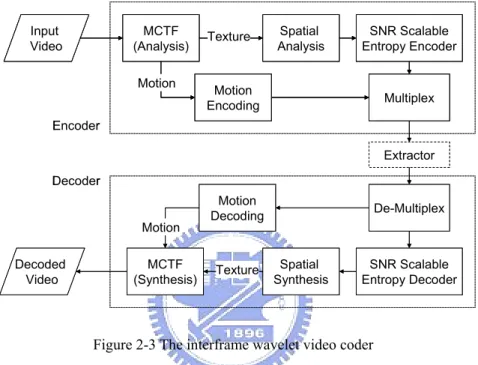
(19) temporal frames are then spatially decomposed by wavelet analysis. The wavelet coefficients are typically coded using arithmetical coding such as embedded zeroblock coding techniques [11]. The architecture of a typical interframe wavelet video coder is shown in Figure 2-3. Basically, there are three major modules in the codec,. temporal. analysis/synthesis,. spatial. analysis/synthesis,. and. entropy. encoder/decoder. We will give a brief overview in the following subsections.. Input Video. MCTF (Analysis) Motion. Texture. Spatial Analysis. SNR Scalable Entropy Encoder. Motion Encoding. Multiplex. Encoder Extractor Decoder. Motion Decoded Video. MCTF (Synthesis). Motion Decoding. Texture. De-Multiplex. Spatial Synthesis. SNR Scalable Entropy Decoder. Figure 2-3 The interframe wavelet video coder. 2.2.1 Temporal Analysis Temporal analysis can be applied by applying high-pass and low-pass filtering along the temporal axis on the same pixel location of each image. Using a simple Haar filter, the temporal subband decomposition would be like Figure 2-4. The low-pass would be a blurred image, a moving average of the original video sequence. The high-pass would be the difference. From the resulting images, we could see that the energy is not compacted very well.. 6.

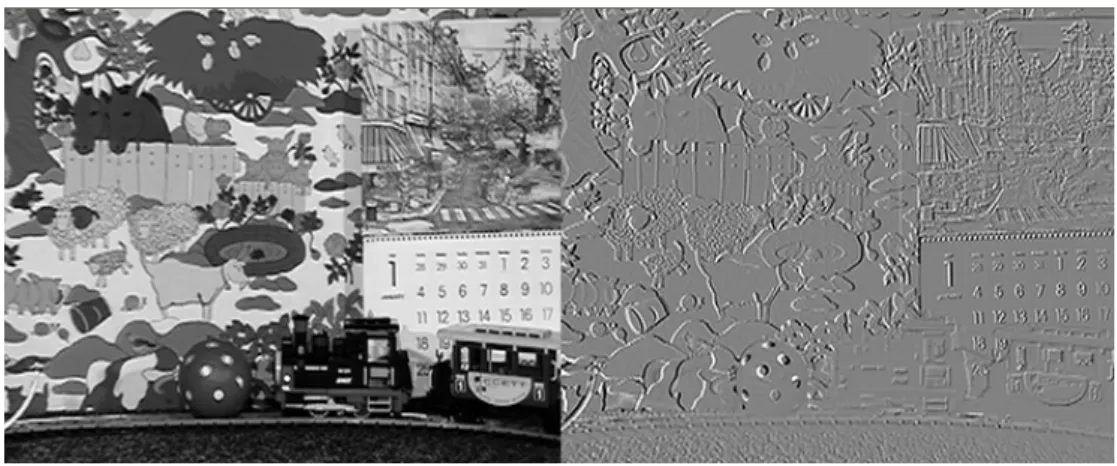
(20) Figure 2-4 Temporal filtered image. (Left: low-pass, Right: high-pass). Motion compensated techniques was first introduced to subband video coding by Kronander [12]. For two consecutive frames, forward block motion estimation is first applied. The forward motion compensated reconstructed frame is then used to do temporal filtering with the second frame to generate subband image. Then the backward block motion estimation is done to create another motion compensated frame. Temporal filtering is done again but using the first frame and the backward motion compensated reconstructed frame. The resulting frames have better characteristics of better energy compaction, like Figure 2-5.. Figure 2-5 Temporal filtered image with motion compensation (Left: low-pass, Right: high-pass). The video coder processes the video sequence in blocks of GOP (group of pictures). Each GOP contains 2n frames, where n equals to the levels of temporal subband decompositions that are done on the GOP. The temporal subband decomposition process is done by first constructing the motion vector map between two consecutive frames, and then motion compensated temporal filtering is applied to the two frames to generate the temporal high-pass frame and the temporal low-pass 7.

(21) frame. After each temporal subband is decomposed, the 2n frame GOP would contain 2n-1 temporal high-pass frames and 2n-1 temporal low-pass frames. The temporal low-pass frames are grouped as another sub-set of GOP, and temporal decomposed again. The decomposition process is iteratively done until there is only one temporal low-pass frame, and a temporal filtering pyramid is constructed, like Figure 2-6.. Video Sequence MCTF. GOP (Group of Pictures) Corresponding to temporal level=4 decomposition. MCTF. MCTF. Temporal Low-pass frame Temporal High-pass frame. MCTF. Frames that remain after temporal decomposition. Figure 2-6 Temporal filtering pyramid [8]. When temporal filtering is done on the GOP, the remaining frames will consist of one temporal low-pass frame, and (1+2+…+2n-1) temporal high-pass frames. These frames, also called residual frames, are then spatially subband decomposed into individual frames by the use of wavelet transform.. 2.2.2 Spatial Analysis The first application of subband coding to images is by Woods and O’neil (1986). The image is separated into spatial subband, encoded separately, and then reconstructed. Primary differences are in how to choose the analysis and synthesis filters. The performance of the filters would affect the rate-distortion performance of 8.

(22) the coding system. Wavelet transform, a special case of subband transform, has become a quite popular method to remove statistical redundancy among the source samples. Wavelet transform is a type of localized time-frequency analysis; therefore, the transform coefficients reflect the energy distribution of the source signal in both space and frequency domains. An example of the transformed (or decomposed) image is shown in Figure 2-7 (Left), the corresponding frequency partition for the decomposed image is shown in Figure 2-7 (Right).. Figure 2-7 Left: Transformed image of the decomposed Lena; Right: Octave-based frequency partition [8]. 2.2.3 Entropy Coder Embedded zeroblock coding is used to code the wavelet coefficients in the interframe wavelet [6]. With the help of two powerful embedded coding techniques – set partitioning and context modeling, the embedded coding algorithm features low computational complexity and high compression efficiency. By exploiting the strong statistical dependencies among the quad-tree nodes built up from the wavelet coefficients, high compression efficiency can be achieved.. 9.

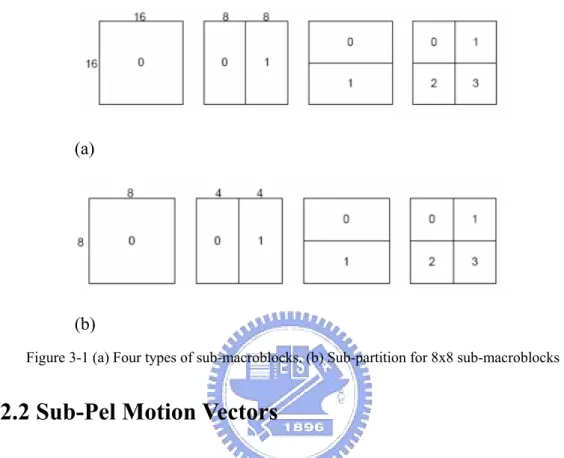
(23) Chapter 3 Interframe Wavelet with H.264/AVC Inter-Prediction Based Motion Compensated Temporal Filtering 3.1 Motivation Our motivation is to improve the motion compensated filtering process in [7]. This is because in the interframe wavelet coding structure, the errors between the original and the reconstruction frames would accumulate along the temporal hierarchy. In addition, the motion-compensated temporal filtered frames are reference pictures in temporal scalability. They are the decoded pictures in the temporally down-sampled playback. Hence, it is critical to have good quality MCTF low-pass frames.. 3.2 H.264/AVC Inter-Prediction Scheme 3.2.1 Tree Structured Motion Compensation The basic unit in AVC motion estimation is the 16x16 macroblock structure. The luminance part of each macroblock can be divided into four types of sub-macroblocks, namely, 16x16, 16x8, 8x16 and 8x8, as illustrated in Figure 3-1(a). The 8x8 10.

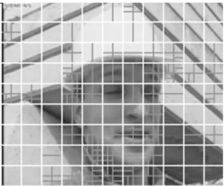
(24) sub-macroblocks can further be partitioned into 8x8, 8x4, 4x8, and 4x4 blocks, as illustrated in Figure 3-1(b).. (a). (b) Figure 3-1 (a) Four types of sub-macroblocks. (b) Sub-partition for 8x8 sub-macroblocks. 3.2.2 Sub-Pel Motion Vectors After completing motion search, the border of the reference picture will be employed for padding, and the full-pel motion estimation will be employed to find the motion vector and the mode with least cost. After the full-pel search, the interpolated picture is used for 1/2 -pel and 1/4 -pel motion search.. 3.2.3 Motion Vector Prediction The motion vector of one block is highly correlated with those of its neighboring blocks. This phenomenon becomes more apparent when the block sizes get smaller. Thus, we can make use of the left, upper-left, upper, and upper-right blocks to reduce the correlation among near-by motion vectors. Figure 3-2 demonstrates an example for mode decision after employing the AVC-based motion estimation.. 11.

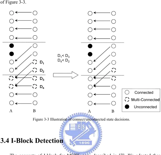
(25) Figure 3-2 An example for mode decision. 3.3 Connection State Decision After applying H.264/AVC motion estimation, we can obtain motion vectors for each frame pair. For the purpose of the temporal decomposition, we need to categorize the connected/unconnected state of each pixel in the frame pair. We call this procedure “connection state decision”. Figure 3-3 is a typical example to illustrate the decision procedure. Before the connection state decision, we can see the left figure in Figure 3-3. The pixels with single motion vector connection are denoted as the straight-line white circles. The pixels with multiple reference pixels in A frame and the related pixels in B frame are so-called multi-connected pixels, and denoted as dotted-line white circles. The others pixels in A are not referenced by any pixel in B, so we call these pixels as unconnected pixels, and they are denoted as black circles. However, the multi-connected pixels in A are not allowed because MCTF can be accomplished along only one motion trajectory for one pixel. Therefore, we need to decide a good motion vector for each multi-connected pixel. It is reasonable that a good prediction has small prediction cost. We use the difference between predicted and referenced pixels as the prediction cost. In the left figure of Figure 3-3, there are two multi-connected pixels in A frames. The corresponding prediction costs of related pixels in B are found and compared. Therefore, each pixel in A has only one corresponding pixel in B to accomplish the MCTF. We can see the connection state changes after state decision in the right figure 12.

(26) of Figure 3-3.. D1. D1< D3 D4< D2. D2 D3 D4 Connected Multi-Connected. A. B. A. B. Unconnected. Figure 3-3 Illustration of connect/unconnected state decisions.. 3.4 I-Block Detection The concepts of I-block for MCTF were described in [7]. We adopted these concepts with some modifications in our MCTF scheme. In the temporal decomposition stage we will do motion estimation first and then do pixel-based state detection. These states could be “connected” or “unconnected” (including the failed ones in multi-connected detection). After that, we decide the sate of each macroblock according to the steps below: Step 1: Unconnected frame detection If the number of connected pixels in these two frames is too small, we think these two frames are not good for MCTF. “Scene change” might happen. So we force the states of whole pixels to “unconnected”. Let Fconnect is a weighting factor between 0 and 1, so the detection criterion is as follows.. 13.

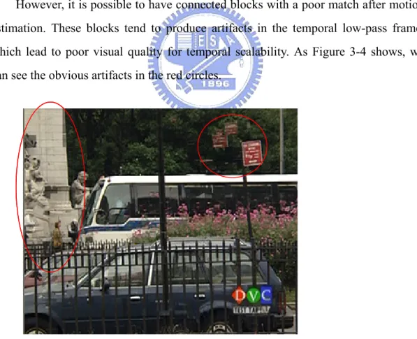
(27) ⎧ MCTF, if{connect ed pixels > F connect * (frame size)}. ⎨ ⎩ MC Only, Otherwise. Step 2: Connected/Unconnected macroblock detection If the frame is not forced to be a unconnected frame in step 1, we will detect the state of each macroblock. Let Fconnect is a weighting factor between 0 and 1, the detection criterion is very similar in step 1:. macroblock state = ⎧Connect, if{connect ed pixels > Fconnect * (macrobloc k size)}. ⎨ ⎩ Unconnect, Otherwise. Step 3: I-block detection However, it is possible to have connected blocks with a poor match after motion estimation. These blocks tend to produce artifacts in the temporal low-pass frame, which lead to poor visual quality for temporal scalability. As Figure 3-4 shows, we can see the obvious artifacts in the red circles.. Figure 3-4 The artifacts of low-pass frame after 4 temporal decomposition.. Therefore, to reduce these artifacts, we hope we can detect these poor match regions, and force their states to ‘unconnected”. Our I-block size is 16x16. According 14.

(28) to Eq. (1), let B[m,n] be the block with connected state at the location (m, n) of the B frame (predicted frame) and A[m-dm, n-dn] be the motion-compensated block with motion vector (dm,dn) in the A frame (reference frame). We compute the variance of these two blocks, and choose the minimum as Vmin. If the mean squared prediction error between these two blocks is larger the threshold F*Vmin, this block is declared as an unconnected block, where F is an adjusting parameter. Based on our experiments, F is taken around 0.7. We will show the visual quality improvement in the experimental results. Let Vmin = min{Var(B[m,n]), Var(A[m-dm, n-dn])}, and the decision is based on:. MSE{B[m, n] - A[m - dm, n - dn]} > F * Vmin. (1). After the above steps, temporal filtering starts. In the prediction stage, we generate the high-pass frame according to Eq. (2). The temporal low-pass frame is generated by Eq. (3) and (4) based on the state of connection of each macroblock. Typically, motion compensation works well on the connected pixels.. (. ). ~ H [m, n ] = B[m, n ] − A[m − d m , n − d n ]. 2. (2). ~ L[m, n] = H [m + d m , n + d n ] + 2 A[m, n]. (3). L[m, n ] = 2 A[m, n ]. (4). 3.5 Motion Cost Function Adjustment The rate-distortion cost function, J= D+ λ*R, is used to decide the best motion vectors in the AVC motion estimation, in which D is the frame difference, and R is the estimated motion vector coding bits. However, as the temporal level increases in MCTF, the energy of temporal low-pass frame is also increased. Therefore, the λ value should be increased to maintain a constant rate-distortion relation at the higher temporal levels. Therefore, the λ value is increased by a factor of W for each additional temporal level. It can be generalized as Eq. (5). The theoretical weighting 15.

(29) factor W is 2 . Therefore, the λ value is increased by a factor of. 2. for each. additional temporal level.. λ(t)= W*λ(t-1) , where t is the temporal level index. (5). 3.6 Bi-Directional MCTF In Eq.(2), H frame is produced by B frame and it’s prediction from A frame. It is only forward prediction. However, the prediction block may find a better match (motion compensation) from the other direction. Since we employ the forward MCTF in the one-directional case, we need to carry out the backward motion compensation. But that will result in an implementation problem. If the backward motion compensation is introduced into the forward MCTF scheme, the future reference frame is required, which means the future GOP data must be ready when the current GOP is encoded/decoded. Therefore, an implementation problem happens. We can simply solve this problem using backward MCTF. To accomplish the backward MCTF with bi-directional MCTF, the forward motion compensation is exploited. The forward motion compensation needs the past GOP data as references, so the mentioned problem can be solved. Figure 3-5 shows the state of connection of each pixel in the backward MCTF scheme.. 16.

(30) Figure 3-5 State of connection of each pixel. After modifying Eq. (2)-(4), we can get Eq. (6)-(8) for backward MCTF. Thus, frame B has both forward and backward motion vectors. The use of bi-directional motion estimation reduces high-pass frame magnitude and thus increases coding efficiency.. (. ). ~ H [m, n ] = A[m, n ] − B [m − d m , n − d n ]. 2. (6). ~ L[m, n] = H [m + d m , n + d n ] + 2 B[m, n]. (7). L[m , n ] =. (8). 2 B [m , n ]. Since we have forward and backward motion vectors for each macroblock, mode decision is necessary. As Figure 3-6 shows, we denote that At and Bt is the tth frame pair at certain temporal level. After bi-directional motion estimation, we can get motion vectors (dx,t, dy,t) and (dx,t-1, dy,t-1) from Bt and Bt-1 respectively. We also can obtain two prediction costs from both directions. The motion vector with minimal prediction cost will be chosen to accomplish the temporal filtering.. 17.

(31) (d x ,t −1 , d y ,t −1 ) Cost t -1. ( d x , t , d y , t ) Cost Bt-1. t. Bt. At. Figure 3-6 Bi-directional motion estimation. 3.7 Experiments and Results In this section, we will show the experiments and results of I-block, motion cost function adjustment, and bi-directional MCTF. The poor match blocks produce artifacts in low-pass frames. After deeper temporal decompositions, these artifacts propagate and cause the significant subjective quality loss. It results in the inaccurate motion prediction in the following temporal decomposition. Figure 3-7 shows the subjective improvement using the I-blocks. The artifacts in the red circles at left image are reduced at right image.. Figure 3-7 The low-pass frame after 4 temporal decompositions: Bus_CIF (Left: without I-Block; right: with I-Block). 18.

(32) I-block detection can improve the subjective quality with very small RD performance loss. Figure 3-8 shows that PSNR is reduced within less than 0.2dB in high bitrates but improved at low bitrates. If the transmission bandwidth is very small, few bitstream remains after extraction. Therefore, the percentage of the low pass signal in the extracted bitstream is large It means the quality of low-pass frame is very important. Hence, the I-block detection can contribute slight improvement at low. 34. PSNR. bitrate. Bus_CIF (15Hz). 33 32 31 30. noI I. 29 28 27 26 25 200. Bitrate 300. 400. 500. 600. 700. 800. 900. 1000. 1100. Figure 3-8 The effect of I-block on RD performance of Bus_CIF sequence. (“noI”: without I-block detection; “I”: with I-block detection). After applying the motion cost function adjustment, we can get better RD performance in all bitrates. However, in our experiments the weighting factor in Eq. (5) needs to be further tuned manually. As Figure 3-9 shows, if W is 2, the RD performance in low rates improves significantly with less than 0.2 dB PSNR loss in high rates, so we choose 2 as our default weighting factor. Figure 3-10 shows the RD performance improvement of Football_CIF sequence.. 19.

(33) MCF adjustment. PSNR. 30 29 28 27 26 25. 1 *sqrt(2). 24. *2 *3. 23 22 21. Bitrate. 20 200. 250. 300. 350. 400. 450. 500. 550. 600. Figure 3-9 Comparison of RD curves with different weighting factors of motion cost function (MCF) (Bus_CIF sequence). Football_CIF. PSNR. 36. 34. 32. 30. 28 26. MCF noMCF. 24. Bitrate 22 300. 500. 700. 900. 1100. 1300. 1500. 1700. 1900. 2100. Figure 3-10 The improvement by motion cost function adjustment of Football_CIF sequence.. Figure 3-11 shows the RD performance comparison between proposed scheme and MC-EZBC. We can find about 1dB PSNR loss at high rates and slight improvement at very low bitrate. However, the subjective quality is comparable. Figure 3-12 shows that the proposed scheme may have better subjective quality even with lower PSNR.. 20.

(34) Football_CIF. PSNR. 45 40 35 30 25. Proposed. 20. MC-EZBC. 15 10 5 Bitrate 0 100. 200. 300. 400. 500. 600. 700. Figure 3-11 RD performance comparison of proposed scheme and MC-EZBC. Figure 3-12 Subjective quality comparison of proposed scheme (left) and MC-EZBC (right). (The 39th frame of Football_CIF at 500kbps.). 21. 800.

(35) Chapter 4 Interframe Wavelet with Motion Information Scalability 4.1 Motivation The interframe wavelet has several advantages over the existing video standards, but it may be improved in a few aspects. In our experiments, we observed that the interframe wavelet does not perform well at low bit-rates. It may be due to the following reasons: First, motion vector information in the bit-stream is for reconstruction at full temporal frame rate and spatial resolution. In fact, the interframe wavelet video coding is designed and optimized for high bit-rates. The coding parameters and strategy may need readjustment when the low rate performance has also some priority. Another cause of the performance loss is that the motion information takes quite a portion of the bit-stream at low bit-rates. For example, the HD-sequence “Harbour” has about 400kbps motion information. In low bit-rate situations, the motion vector cannot even fit into the total bit budget. The high motion information bit-rate is mainly due to the fact that at higher levels of the temporal pyramid decomposition, the appropriate motion vector range is larger. In a GOP with four-level temporal decomposition, the motion information of the highest level pair would need approximately three times more bits than the lowest level pair. Motion vector prediction has than been proposed to compress the size of the motion information, but 22.

(36) still the total motion information is huge [14]. When the low bit-rate and spatial scalability are together required, the performance of the interframe wavelet drops significantly. This is mainly because of the fact that the motion information does not have spatial scalability built in it. For example, a bit-stream containing of a coded sequence of spatial resolution of 720x480, the spatially down-scaled resolution of 360x240 truncated bit-stream still contains all the motion information that used to construct the 720x480 size images. In the following section, we propose a motion information partitioning scheme that can improve the performance of interframe wavelet video coding at low bit-rates. 4.2 Motion Information Partitioning In [15], Hang and Tsai proposed the motion information scalability for MC-EZBC. In this thesis, we extend this concept with some modifications to partition the motion information generated by the AVC interframe-prediction in MCTF. The wavelet coefficient information in the conventional interframe wavelet coding scheme has spatial, temporal and SNR scalability but the motion information can not be partitioned for the cases of spatial and SNR scalability. If the required bitrate is very slow, the extractor (puller) may fail to extract the bitstream because the motion information bits are larger than the specified bits. Also, at low rates, we may want to save some bits from motion information and use these bits for wavelet coefficients to achieve acceptable quality. Therefore, we partition motion information after motion estimation. The basic idea is to partition the motion information into multiple “motion layers”. Each layer records the motion vectors with a specified accuracy. The lowest layer denotes a rough representation for the motion vectors and the higher layers are used to improve the accuracy. Particularly, different layers are coded independently so that the motion information can be truncated at the layer boundary. In AVC interframe-prediction, the basic unit in prediction is the macroblock of 23.

(37) 16x16. Each macroblock could be the combinations of 16x16, 16x8, 8x16, 8x8, 8x4, 4x8, and 4x4, and the corresponding motion vectors have 1/4-pixel accuracy. We denote that MVi is the motion vector in motion layer index i, and Modei is the best prediction mode. We partition the motion vectors according to the steps below. Step 1: Do 16x16 block size motion search with integer-pixel accuracy. In this step, the base-layer motion information is obtained. Since the first motion layer records the rough motion vectors. We only allow the macroblock size motion estimation with integer-pixel accuracy, so Mode0 can only be 16x16. Besides, to simplify the motion partitioning scheme with bi-directional motion estimation, the direction of motion vectors in the following motion layers are determined in Step 1. Step 2: Do 16x16 and 8x8 block size motion search with 1/2- pixel accuracy. The first enhanced motion layer is derived in Step 2 to refine the base-layer motion information. The more detailed motion vectors are produced in this step, so Mode1 can be {16x16, 16x8, 8x16, 8x8} with half pixel accuracy. Besides, we use the base-layer motion vectors to predict the current motion vectors. The difference between current motion vectors and the base-layer ones are the first enhanced motion layer. If we denote the obtained motion vector in this step as MV, the output residue vector MV1 is (MV- MV0*2). Step 3: Do all sub-block size motion search with 1/4- pixel accuracy. The further refined motion vector is obtained in this step. We allow the whole possible mode with 1/4 pixel accuracy to get the finest motion vector, so the Mode2 can be {16x16, 16x8, 8x16, 8x8, 8x4, 4x8, 4x4}. We also use the previous motion layers to prediction the current motion vectors. The difference between these motion vectors and the base-layer plus the first-enhancement-layer is as the second enhancement layer motion vectors. MV is denoted as the obtained motion vector in this step, so the output residue vector MV2 is MV2 – (MV1 + MV0*2)*2 Step 4: Encode the above three layers motion information using CABAC separately. 24.

(38) After all motion layers are ready, they are encoded with CABAC independently. The motion information can be truncated at the layer boundary according to the spatial size or bitrate requirement. As Figure 4-1 shows, the original motion vectors are partitioned into three layers. Each frame of motion information in the temporal decomposition is divided into base layer and enhancement layers as described earlier. Original. Proposed. Base layer Original ¼ pixel accuracy 1st enh. layer. Proposed Base layer: integer pixel accuracy 1st enh. layer: ½ pixel accuracy 2nd enh. layer: ¼ pixel accuracy. 2nd enh. layer. Figure 4-1 The base and enhancement motion layers. 4.3 Motion Information Scalability Therefore, the entire motion vector information is organized into groups as shown in Figure 4-2. The base layers of all temporal levels are needed to reproduce the full-temporal resolution sequence. Hence, they (base layers) are the highest priority motion vector information data.. 25.

(39) B E. Temporal Level 1 Temporal Level 2 Temporal Level 3. B E. B E. B E. B E. B E. B E. B E. B E. B E. B E. B E. B E. B E. B E. Temporal Level 4. Figure 4-2 Motion information of a GOP If the required bitrate is too small, the extractor will drop one or two enhancement layers according to the conditions. Besides, if the user wants to extract the spatially down-sampled bitstream, the extractor can also drop proper enhancement layers. When the codec scalability number is small, we can reduce the enhancement layers into one to save bits in encoding motion vectors.. S2 1-pixel accuracy. 1-pixel accuracy. S1. S1. 1/2-pixel accuracy. 1/4-pixel accuracy. 1/2-pixel accuracy. S0. 1/4-pixel accuracy. (a). S0. (b). Figure 4-3 Different resolution with different number of motion layers: (a) for two spatial resolutions S0 and S1; (b) for three spatial resolutions S0, S1, and S2.. Here we take Figure 4-3 as an example. We denote the original spatial resolution 26.

(40) is S0, S1= S0/4, and S2= S1/4. And we partition the motion information into 3 motion layers. In Figure 4-3 (a), if we need two spatial resolutions S0 and S1, we can extract the top two motion layers for S1 and all motion layers for S0. Besides, the motion vectors are with 1/4-pixel accuracy both in S0 and S1. The similar concept can be applied for three spatial resolution case, as Figure 4-3 (b) shows. Figure 4-4 is the basic operation element in reconstructing pictures in the interframe temporal hierarchy. Frames A and B are reconstructed using frames L and H. Frame A is roughly the sum of the original frame L and the motion compensated version of frame H. The drift comes from the motion-compensated portion of frame H because now the motion vectors are truncated. Frame B is essentially the sum of the original frame H and the motion compensated drifted copy of frame L. Because frame L usually has a much larger power than frame H, the magnitude of drift errors in frame A is much higher than that of frame B. These drift errors propagate from the higher temporal levels to the lower levels.. H. Motion C ompens a. L tion. tion ompensa Motion C. B. A. Figure 4-4 The temporal synthesis process. 4.4 Experiments and Results In Figure 3-11, we can observe that the RD curve can not extend to low rates because the “pull” process fails. The reason of the failure is the large motion 27.

(41) information. Therefore, we partition the motion information into two layers and truncate one motion layer at low rates properly. As Figure 4-5 shows, we can get significant RD improvement at very low bitrates, while the RD performance of MC-EZBC drops fast because of the large motion information. We can also see Figure 4-6 and Figure 4-7. The subjective quality is acceptable at low bitrates. PSNR. 35. Football_CIF. 30. 25. 20. 15. Proposed. 10. MC-EZBC. 5 Bitrate 0 100. 120. 140. 160. 180. 200. 220. 240. Figure 4-5 The proposed motion information partitioning scheme v.s. MC-EZBC in low bitrates.. Figure 4-6 The 15th frame of Football_CIF at 128k with motion information partitioning. 28.

(42) Figure 4-7 The 238th frame of Football_CIF at 196kbps with motion information partitioning. (Left: proposed scheme. Right: MC-EZBC). In the MPEG scalable video coding call-for-proposal [18], the MPEG committee specifies three main test conditions that define the test points for temporal, spatial and SNR scalabilities. For the CIF size sequences, there are two test conditions, test 2a and test 2b. To achieve the best performance, we manually tune all parameters. Table 1 and Table 2 show the detailed settings. Under very low bitrate conditions, we truncate motion layers properly to prevent extraction failure. Table 1 Parameters for Test 2a.. Mobile_CIF. Encoded. Motion. Extracted. Extracted. Extracted. Extracted. GOP size. Search. Spatial. Frame. Bitrate. Motion. Range. Resolution. Rate(fps). (kbps). Layers. 16. 176x144. 7.5. 64. 1. 176x144. 15. 128. 1. 352x288. 15. 256. 2. 352x288. 15. 512. 2. 352x288. 30. 1024. 2. 176x144. 7.5. 64. 1. 176x144. 15. 128. 1. 352x288. 15. 256. 2. 352x288. 15. 512. 2. 352x288. 30. 1024. 2. 8. (300 frames). Football_CIF (260 frames). 4. 16. 29.

(43) Table 2 parameters for Test 2b. Encoded. Motion. Extracted. Extracted. Extracted. Extracted. GOP size. Search. Spatial. Frame. Bitrate. Motion. Range. Resolution. Rate(fps). (kbps). Layers. 16. 176x144. 7.5. 48. 1. 176x144. 15. 64. 1. 352x288. 15. 128. 2. 352x288. 15. 256. 2. 352x288. 30. 512. 2. 176x144. 7.5. 48. 1. 176x144. 15. 64. 1. 352x288. 15. 128. 2. 352x288. 15. 256. 2. 352x288. 30. 512. 2. Bus_CIF. 8. (150 frames). Foreman_CIF. 4. 16. (300 frames). Figure 4-8 shows the experimental results for all test conditions. In some cases in Figure 4-8, the GOP size affects the coding performance significantly. The reason is the “scene change” problem. If “scene change” happens, the coding performance of MCTF degrades rapidly in the corresponding GOP due to the inefficient temporal decomposition. Some possible solutions are suggested in the next chapter.. 30. Mobile (CIF). PSNR. 35. 25 20 GOP= 8 GOP= 4. 15 10 5. Test Points. 0 176x144_7.5_64. 176x144_15_128. 352x288_15_256. (a). 30. 352x288_15_512. 352x288_30_1024.

(44) 33. PSN R. 34. Football (CIF). 32 31 30 GOP= 8 GOP= 4. 29 28 27 26. Test Points. 25 176x144_7.5_64. 176x144_15_128. 352x288_15_256. 352x288_15_512. 352x288_30_1024. (b) 40. Foreman (CIF). PSNR. 35 30 25 20. GOP= 8 GOP= 4. 15 10 5. Test Points. 0 176x144_7.5_48. 176x144_15_64. 352x288_15_128. 352x288_15_256. 352x288_30_512. (c) 35. Bus (CIF). PSNR. 30 25 20. GOP= 8 GOP= 4. 15 10 5. Test Points. 0 176x144_7.5_48. 176x144_15_64. 352x288_15_128. 352x288_15_256. 352x288_30_512. (d) Figure 4-8 RD curves for Test 2a and Test 2b (a) Mobile_CIF (b) Football_CIF (c)Foreman_CIF and (d)Bus_CIF. 31.

(45) For some test points, although the data extraction (“pull”) process can run successfully, the percentage of motion information is still too high and it may still result in quality loss. After we truncate motion layers properly, we can decrease the percentage of motion information. In Figure 4-9, we see that the proposed motion partitioning scheme produces better visual quality due to the reduction of motion information.. (a). (b) Figure 4-9 Subjective quality comparison of proposed scheme (left) and MC-EZBC (right). (a) the 77th frame of Mobile at {15fps, QCIF, 128kbps}. (b) the 31st frame of Mobile at {7.5fps, QCIF, 64kbps}. The proposed algorithm can provide acceptable video quality at very low bit rates, especially for high-motion cases. However, if not all the motion vectors are used in reconstruction, the “drifting errors” would occur. That is, the residual image data calculated at the encoder are based on the complete set of motion vectors but only “partial” motion vectors are available at the decoder if they are truncated. We can see the PSNR distribution along frame index in Figure 4-10. There are some peak PSNR values in this figure. These peak values appear periodically, and the periodic is exactly the GOP size, that is, the error drifts within the local GOP. This problem needs to be further studied. 32.

(46) Football_CIF @ 196kbps (1/2 M.I. Layer) PSNR. 40 35 30. 25 20 Frame Index. 15 1. 11 21 31 41 51 61 71 81 91 101 111 121 131 141 151 161 171 181 191 201 211 221 231 241 251. Figure 4-10 PSNR distribution along frame index for Football_CIF at 196kbps with partitioning 1 motion layer.(GOP size = 16). 33.

(47) Chapter 5 Conclusion and Future Work 5.1 Conclusion In this thesis, we propose an enhanced coding scheme for motion compensated temporal filtering to improve the existing interframe wavelet coding algorithm (MC-EZBC). We modify the motion estimation syntax/scheme specified in AVC to fit into the motion compensated temporal filtering (MCTF) structure. Various additional techniques such as I-block, bi-directional motion estimation and λ-value adjustment are incorporated. Moreover, we propose a motion information partitioning technique for AVC interframe-prediction to further improve coding performance at low rates. The diagram of the modified MCTF scheme is shown in Figure 5-1. Simulation results indicate that this new motion estimation algorithm improves the subjective image quality significantly at low bit rates. AVC Interframeprediction. Connect / Unconnect Detection. 2 or 3 layers of Motion vectors. I-block Detection. Temporal Filtering. L, H frame Status of MB (Connect/ Unconnect). CABAC Coding. Figure 5-1 Diagram of temporal information processing. 34. 2 or 3 layers Encoded Mode/MV.

(48) 5.2 Future Work Based on our experiences, many issues can be further investigated. In temporal filtering, the quality of low-pass frame is very important. The quality of low-pass frame has a strong impact on the coding efficiency of temporal decomposition. Hence, how to do accurate prediction is an important research topic. The other problem is “scene change”. To reduce the loss due to “scene change”, the concept of intra prediction and adaptive GOP coding scheme can be further studied. Moreover, because of the mismatch between the truncated motion information and the residue signal, the error drifting problem is another issue for further study. A better rate-control algorithm is very desirable. That is, we like to have a better rate control to balance the RD relation between motion information and texture coded data. Because of the extra distortion due to motion information partitioning (drifting), this rate control problem is quite sophisticated and thus is very challenging.. 35.

(49) References [1] T. Wiegand, G. J. Sullivan, G. Bjontegaard, and A. Luthra, “Overview of the H.264/AVC Video Coding Standard”, IEEE Trans. Circuits Syst. Video Technol., vol. 13, pp. 560–576, July 2003. [2] B. G. Haskell, A. Puri, and A. N. Netravali, Digital Video: An Introduction to MPEG-2. New York: Chapman & Hall, Sept. 1996. [3] R. Aravind, M. R. Civanlar, and A. R. Reibman, “Packet loss resilience of MPEG-2 scalable video coding algorithm,” IEEE Trans. Circuits Syst. Video Technol., vol. 6, pp. 426–435, Oct. 1996. [4] W. Li, “Overview of fine granularity scalability in MPEG-4 video standard,” IEEE Trans. Circuits Syst. Video Technol., vol. 11, pp. 301-317, Mar. 2001. [5] J.-R. Ohm, “Three-dimensional subband coding with motion compensation,” IEEE Trans. Image Processing, vol. 3, no. 5, pp. 559–571, Sep. 1994. [6] S.-T. Hsiang and J. W. Woods, “Embedded video coding using invertible motion compensated 3-D subband/wavelet filter bank,” Signal Processing: Image Communications, vol. 16, pp. 705–724, May 2001. [7] P. Chen, Fully scalable subband/wavelet coding, Ph.D. thesis, Rensselaer Polytechnic Institute, Troy, New York, May 2003. [8] S. S. Tsai, Motion information scalability for interframe wavelet video coding, MS thesis, National Chiao Tung University, Hsinchu, Taiwan, R.O.C., Jun. 2003. [9] J.W. Woods, “"AHG on Digital Cinema Video Coding Technology”, ISO/IEC JTC1 SC29/WG11 doc. No. M7645, Pattaya, December 2001 [10] P.S. Chen, J.W. Woods, “Comparison of MC-EZBC and H.26L TM8 on Digital Cinema Test Sequences”, ISO/IEC/JTC1 SC29/WG11 doc. No. m8130, Cheju Island, March 2002 [11] S.T. Hsiang and J.W. Woods, “Embedded image coding using zeroblocks of subband-wavelet coefficients and context modeling”, in Proceedings of IEEE International Symposium on Ciruits and Systems, vol. 3:5, pp662-665, May 2000. [12] T. Kronander, “Motion compensated 3-dimensional wave-form image coding”, 36.

(50) International Conference on Acoustic, Speech, and Signal Processing, vol. 3, pp1921-1924, 1989 [13] T. Rusert, et al., Recent Improvements to MC-EZBC, ISO/IEC/JTC1 SC29/WG11 No. M9232, Dec. 2002. [14] D.S. Turaga, M.V.d Schaar, B. Pesquet-Popescu, “Differential motion vector coding in the MCTF framework”, ISO/IEC/JTC1 SC29/WG11 doc. No. m9035, Shanghai, October 2002 [15] H.-M. Hang, S. S. Tsai, and Tihao Chiang, “Motion information scalability for MC- EZBC”, ISO/IEC/JTC1 SC29/WG11 doc. No. M9756, July 2003. [16] Call for proposals on scalable video coding technology, ISO/IEC JTC1/SC29/WG11 MPEG2003/N6193, Dec. 2003 [17] B. Pesquet-Popescu, V. Bottreau, “Three-dimensional lifting schemes for motion compensated video compression,” Int’l Conf. Acoustic, Speech, and Signal Processing, vol. 3, pp. 1793–1796, 2001. [18] Call for proposals on scalable video coding technology, ISO/IEC /JTC1 SC29/WG11 MPEG2003/N6193, Dec. 2003.. 37.

(51) 作者簡歷蔡家揚 (Chia-Yang Tsai): 1979 年 2 月 18 日生於台北縣。2001 畢業於國立交通大學電子工程學系，同年進交大電子所就讀碩士班，並於 2003 年直攻博士班，2005 年轉回碩士班取得碩士學位。研究範圍與興趣主要為視訊編碼研究。. 38.

(52)