Embedding Edge-Disjoint Spanning Trees on the Alternating Group Graphs

全文

(1)International Computer Symposium 2002, Workshop on Computer Systems. Embedding Edge-Disjoint Spanning Trees on the Alternating Group Graphs Chin-Tsai Lin (林錦財)* Assistant Professor Department of Information Management, Kun-Shan University of Technology. Abstract In this paper we construct a graph that consists of the maximum number of directed edge-disjoint spanning trees on the alternating group graph. The paths that route from the common root node to any given node through different spanning trees are node-disjoint. This graph can be used to derive fault tolerant algorithms for the broadcasting and scattering problems under the all port communication model. Keywords: Interconnection networks, alternating group graphs, node-disjoint paths, edge-disjoint spanning trees *Correspondance: 台南縣永康市 710 忠義街 10 巷 1 號, Taiwan Tel.: Fax.: E-mail:. (06) 311-2107 (0921) 217-922 (06) 273-2726 ctlin@mail.ksut.edu.tw jench1@seed.net.tw.

(2) International Computer Symposium 2002, Workshop on Computer Systems. Embedding Edge-Disjoint Spanning Trees on the Alternating Group Graphs Chin-Tsai Lin Department of Information Management, Kun-Shan University of Technology Taiwan, Republic of China. Abstract In this paper we construct a graph that consists of the maximum number of directed edge-disjoint spanning trees on the alternating group graph. The paths that route from the common root node to any given node through different spanning trees are node-disjoint. This graph can be used to derive fault tolerant algorithms for the broadcasting and scattering problems under the all port communication model. Keywords: Interconnection networks, alternating group graphs, node-disjoint paths, edge-disjoint spanning trees. 1.. Introduction Jwo, Lakshmivarahan and Dhall [18] proposed Cayley graphs based on the alternating. groups as a topology for interconnecting processors in parallel computers. With respect to contention problem for general routing, it has been shown that alternating group graphs perform better than the star graphs and are close to the hypercube. The alternating group graphs are defined as follows. Let gi+ denote the permutation (1 2. i), gi- denote (1 i 2). Let Ω={gi+| 3 ≤ i ≤ n}∪{gi-|3 ≤ i ≤ n}. It is well known that Ω is a 1.

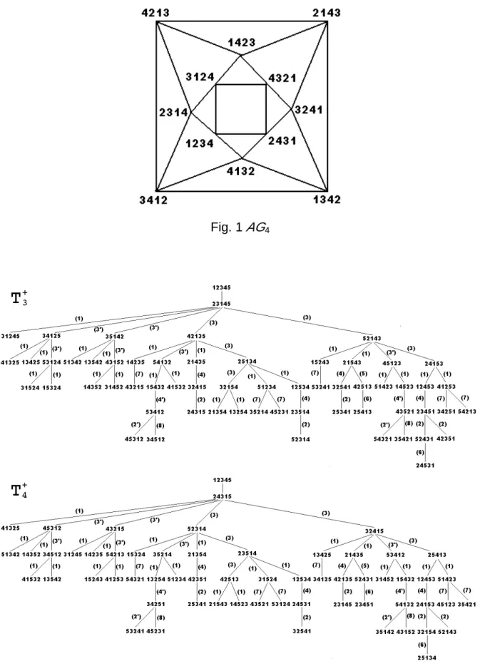
(3) International Computer Symposium 2002, Workshop on Computer Systems. generator set for the set of all even permutations of n symbols, denoted by An. Definition 1. An alternating group graph on n symbols, denoted by AGn = (Vn, En), is an undirected graph with n!/2 nodes, in which Vn is the set of n!/2 even permutations. En = {(p,. q)|p, q∈ An, q= p⋅ h, for h∈Ω}. Fig. 1 shows the AG4 graph. It can be verified that gi+⋅gi+=gi-, gi-⋅gi-=gi+, (gi+)-1= gi- and (1 2)⋅gi+⋅(1 2) = gi-, for 3 ≤ i ≤ n. The diameter of AGn is 3(n-2)/2 and the connectivity is optimal, i.e., equal to the degree 2(n-2). Alternating group graphs have received considerable attention. In [19], Lai and Tsay presented algorithm for all-port all-to-all broadcasting and single-node scattering whose time performances are one step more than the lower bounds. Hung and Huang [15] also introduced an optimal one-port one-to-all broadcasting algorithm on alternating group graphs. Yang et al. [23] introduced a method to explore a set of edge-disjoint paths between any two nodes. In [20], it has been shown that the fault diameter of an alternating group graph is no more than the original diameter by one. Cheng and Lipman [5] have shown that the alternating group graphs are a subclass of arrangement graphs. Day and Tripathi [9] introduced schemes for constructing node-to-node disjoint paths in the arrangement graphs. Another scheme for constructing node-to-node disjoint paths is given in [21]. In this paper, we introduce a scheme for constructing on AGn 2(n-2) directed. edge-disjoint spanning trees (EDSTs). This is the maximum number of edge-disjoint spanning trees that can be constructed on AGn, since the degree of AGn is 2(n-2). The depth of the. 2.

(4) International Computer Symposium 2002, Workshop on Computer Systems. EDSTs graph we construct differs from the minimum possible depth by a small constant. The root node of EDSTs has 2(n-2) node-disjoint paths to each one of the other nodes, one path through each of the 2(n-2) edge-disjoint spanning trees. Similar graphs have been previously constructed on other interconnection networks, such as the binary hypercube [16], the cube-connected-cycles (CCC) [13], and the star graphs [12]. The construction of the EDSTs graph is equivalent to the problem of exploiting the disjoint paths between a node s and all the other n!/2–1 nodes of AGn. Using the EDSTs graph we can derive fault tolerant algorithms for the single-node and multimode broadcasting, and for the single-node and multinode scattering problem on AGn as in [12]. The remaining of the paper is organized as follows. In the next section, we will introduce the notations and definitions that are throughout the paper. Section 3 presents the scheme of embedding 2(n-2) directed edge-disjoint spanning trees. Conclusions are finally drawn in section 4. 2.. Notations and Definitions We now define the rotation operation that is important for constructing the 2(n–2). directed edge-disjoint spanning trees. Definition 2. Let us define a bijection r from the set {1, 2, … ,n} to itself as follows:. i,. if i = 1 or 2. r (i) = ((i-2) mod (n-2)) + 3, otherwise, (notice that r maps symbols 1 and 2 to themselves and the remaining symbols as follows: 3 →. 3.

(5) International Computer Symposium 2002, Workshop on Computer Systems. 4 →… → n-1 → n → 3). The rotation of a node p of AGn is defined to be the node:. R(p) = r (p1)r (p2)r (pn)r(p3)… r (pn-1) or equivalently R(p) = p′ so that p′r (i) = r (pi), 1 ≤ i ≤ n. This means that the position of each symbol of p and the symbol itself are mapped through r . For example, R(4132) = 3124 and R(4321) = 3412. Notice that R(gi+) =. g ((+ i − 2 ) mod(n-2))+3 and R(gi-) = g ((− i − 2 ) mod (n-2))+3. By rotation of a network we mean that rotation is applied to each node of the network. The rotation operation is an automorphism on AGn that possesses the following properties. 1. It maps the identity node to itself. As an extension to this, nodes p and R(p) are always at the same distance from the identity node. 2. Let (v, u) be an edge and u = v⋅giσ. Then (R(v), R(u)) is an edge of generator. g σ((i − 2 ) mod(n-2))+3. (σ denotes the sign + or -.) The conjugation operation is also important for constructing the 2(n–2) directed edge-disjoint spanning trees. Definition 3. The conjugation of a node p of AGn is defined to be the node (1 2)⋅p⋅(1 2). 3.. The edge-disjoint spanning trees In this section we construct the 2(n-2) directed edge-disjoint spanning trees graph,. rooted at the identity node of AGn. The spanning tree rooted at the neighbor of the identity node over generator giσ, node giσ, is denoted by Tiσ. Each spanning tree includes all nodes of. AGn except the identity node. The reverse-direction spanning tree of Tiσ is a rendezvous result. 4.

(6) International Computer Symposium 2002, Workshop on Computer Systems. of the disjoint paths whose last generator is (giσ)–1 from each one of the other nodes to the identity node. Since the alternating group graphs are symmetric, the EDSTs graph can be easily translated into that rooted at any other node. Before proceeding to description of the spanning trees algorithms, we need the following definition. Definition 4. For each node p (excluding the identity node and its neighbor), we define w1 and w2 as follows: 1.If the cycle structure of p is (x1 x2 … xt 1)(2)… or (x1 x2 … xt 1 2)… , t > 1, we define w1 = x1. For example, for node p = 42351 = (4 5 1)(2)(3) of AG5, we have w1 = 4. 2.If the cycle structure of p is (x1 1)(2)… or (x1 1 2)… , we define w1 to be the first position in. p, among x1+1, … , n, 3, … , x1–1 that does not include its correct symbol. If w1 cannot be found, we let w1= 0 and pw1 = 0. For example, for node p = 52431 = (5 1)(2)(3 4) of AG5, we have pw1 = p3 = 4. For node 25341 = (5 1 2)(3)(4) of AG5, we have w1 = pw1= 0. 3.If the cycle structure of p is (y1 y2 … ys 2)(1)… or (y1 y2 … ys 2 1)… , s > 1, we define w2 = y1. For example, for node p = 31452 = (3 4 5 2 1) of AG5, we have w2 = 3. 4.If the cycle structure of p is (y1 2)(1)… or (y1 2 1)… , we define w2 to be the first position in. p, among y1+1, … , n, 3, … , y1–1 that does not include its correct symbol. If w2 cannot be found, we let w2= 0 and pw2 = 0. For example, for node p = 13254 of AG5, we have pw2 = p4 = 5. For node 41325 = (4 2 1)(3)(5) of AG5, we have w2 = pw2 = 0. 5.If the cycle structure of p is (x1 x2 … xt 1)(y1 y2 … ys 2)… or (x1 x2 … xt 1 y1 y2 … ys 2)… , s ≥. 5.

(7) International Computer Symposium 2002, Workshop on Computer Systems. 1, t ≥ 1, we define w1 = x1 and w2 = y1. For example, for node p = 43521= (3 5 1 4 2) of AG5, we have w1 = 3 and w2 = 4. We now describe an algorithm, Parent(p, Tiσ), that for given node p (excluding the identity node and its neighbors) computes the parent node of p in each one of the spanning tree Tiσ, 3 ≤ i ≤ n. In what follows, by fi(p) we denote the parent of node p in spanning tree Tiσ. Since the first two symbols is determinate if the other symbols are known, an even permutation p= p1p2… pn can be represented by {p1, p2}p3… pn or {p2, p1}p3… pn without ambiguity. Algor ithm Parent(p, Tiσ) { if (σ==+) { // 1 is at position i right before reaching the identity node (1) if (p=={1, z}p3… pn) {fi(p) ={z, pi}p3… pi-11pi+1… pn;}. // z may be 2 or y1. else if (p=={2, x1}p3… pn) {. k = p–1(1); (2). if (i≠k and i≠ pw1 and i≠ x1) {fi(p) ={i, 2}p3… pn;}. (3). else if (i==k) {fi(p) ={pw1, 2}p3… pw1-1x1pw1+1… pn;}. (4). else if (i==x1) {fi(p) ={1, 2}p3… pk-1x1pk+1… pn;} else if (i==pw1) {. (5) (6). if (x1==k) {fi(p) ={1, 2}p3… pk-1x1pk+1… pn;} else {fi(p) = {k, 2}p3… pn;} } // end of if (p=={2, x1}p3… pn). 6.

(8) International Computer Symposium 2002, Workshop on Computer Systems. else if (p=={x1, y1}p3… pn) {. // x1, y1 are as those stated above. k1 = p–1(1); k2 = p–1(2); (2’). if (i∉{k1 , pw1 , x1}and i∉{y1, y2, … , ys}) {fi(p) ={y1, i}p3… pn;}. (3’). if (i==k1) {fi(p) ={pw2, x1}p3… pw2-1y1pw2+1… pn;}. (4’) (6’) (7) (8) (9). else if (i==x1) {fi(p) ={y1, 1}p3… pk1-1x1pk1+1… pn;} else if (i==pw1) {fi(p) ={y1, k1}p3… pn;} else if (i==k2) {fi(p) ={1, x1}p3… pk1-1y1pk1+1… pn;} else if (i==y1) { fi(p) ={y1, k2}p3… pn;} else {fi(p) ={y1, i}p3… pn;} } // end of if (p=={ x1, y1}p3… pn). } // end of if (σ==+) if (σ==–) { // 2 is at position i right before reaching the identity node; // It is the conjugation of the case σ==+. (1) if (p=={2, z}p3… pn) {fi(p) ={ z, pi}p3… pi-12pi+1… pn;}. // z may be 1 or x1. else if (p=={1, y1}p3… pn) {. k = p–1(2); (2). if (i≠k and i≠ pw2 and i≠ y1) {fi(p) ={i, 1}p3… pn;}. (3). else if (i==k) {fi(p) ={pw2, 1}p3… pw2-1y1pw2+1… pn;}. (4). else if (i==y1) {fi(p) ={1, 2}p3… pk-1y1pk+1… pn;} else if (i==pw2) {. 7.

(9) International Computer Symposium 2002, Workshop on Computer Systems. (5). if (y1==k) {fi(p) ={1, 2}p3… pk-1y1pk+1… pn;} else {fi(p) = {k, 1}p3… pn;}. (6). } // end of if (p=={1, y1}p3… pn) else if (p=={x1, y1}p3… pn) {. // x1, y1 are as those stated above. k1 = p–1(1); k2 = p–1(2); (2’). if (i∉{k2, pw2, y1} and i∉{x1, x2,… , xt}) {fi(p) ={x1, i}p3… pn;}. (3’). else if (i==k2) {fi(p) ={pw1, y1}p3… pw1-1x1pw1+1… pn;}. (4’). else if (i==y1) {fi(p) ={x1, 2}p3… pk2-1y1pk2+1… pn;}. (6’) (7). else if (i==pw2) {fi(p) ={x1, k2}p3… pn;} else if (i==k1) {fi(p) ={2, y1}p3… pk2-1x1pk2+1… pn;} else if (i==x1) {fi(p) ={x1, k1}p3… pn;}. (8). else {fi(p) ={x1, i}p3… pn;}. (9). } // end of if (p=={ x1, y1}p3… pn) } // end of if (σ==–) } // end of algorithm. For example, the EDSTs graph on AG5 are shown in Fig.2. The following lines illustrate the usage of rules (6’) and (9) in the case p = 43156287 = (3 1 4 5 6 2) (7 8) through T5– and T5+ respectively on AG8: ( 6 ') ( 2 ') ( 4 ') (1) T5–: 43156287  → 36154287  → 53164287  → 32164587 → 43162587→…. (9) ( 8) ( 4 ') (1) T5+: 43156287 → 54136287 → 65134287  → 16534287 → 64531287→… .. 8.

(10) International Computer Symposium 2002, Workshop on Computer Systems. Theorem. The Parent(p, Tiσ) algorithm defines a spanning tree, rooted at the node giσ. The 2(n–2) spanning trees constructed by the Parent algorithm possess the following properties: 1) If all the edges of the spanning trees are directed from parent to children nodes, these spanning trees are edge-disjoint. Consequently, the EDSTs graph with node 12… n as the common root contains all edges of AGn except those edges that are directed towards node 12… n. 2) The identity node has 2(n–2) disjoint paths to each other node of AGn, one path through each one of the 2(n–2) spanning trees. The lengths of these paths differ from the shortest possible lengths by a small additive constant. 3) The depth of the EDSTs graph is less than or equal to 3(n – 2)/2+4, which is optimal to within a small additive constant. This constant is less than or equal to 3. 4) Each spanning tree can be derived from its preceding one, by the application of a rotation or conjugation. From the properties of the rotation and conjugation operations, we conclude that all the spanning trees are isomorphic. Proof: We prove each of the properties separately. 1) It is sufficient to prove that the parent of a node p in each one of the spanning trees, is a different one of its neighbor nodes. Four cases of p are distinguished: i) p = {1, 2}p3… pn. Its parent in Ti+, fi(p) ={2, pi}p3… pi-11pi+1… pn, is derived from moving 1 to position i and its parent in Ti–, fi(p) ={1, pi}p3… pi-12pi+1… pn, is derived from moving 2 to position i, for 3 ≤ i ≤ n. Clearly, the parent of the node in each one. 9.

(11) International Computer Symposium 2002, Workshop on Computer Systems. of the 2(n–2) spanning trees is a different one of its neighbor nodes. ii) p = {1, y1}p3… pn, where y1 ≠ 2. Its parent in Ti+, fi(p) ={y1, pi}p3… pi-11pi+1… pn, is derived from moving 1 to position i, while its parent in Ti– has symbol 1 at one of the first two positions and y1 at some position j, 3 ≤ j ≤ n. Clearly, the parent nodes in Ti+, are different. The parents in Ti– are again different neighbors of p because the j’s are different.. p: pw2= p–1(2) p: pw2≠ p–1(2) and y1≠ p–1(2) Ti–: i = p–1(2) Rule (3); j = p–1(pw2) Ti–: i = y1 Rule (3) Rule (4); j = p–1(2) – –1 Ti : i = pw2 Rule (5); j = p (2) Rule (3) Rule (6); j = p–1(p–1(2)) Ti–: i = other Rule (2); j = p–1(i) p: y1= p–1(2). iii) p = {x1, 2}p3… pn, where x1 ≠ 1.The proof is similar to the case b) except by conjugation. iv) p = {x1, y1}p3… pn, where {x1, y1} ≠ {1, 2}. It can be verified that the parent nodes in. Ti+ by rules (2’), (4’), (6’), (8) and (9), and those in Ti– by rules (3’) and (7), y1 is at one of the first two positions and the positions of symbol x1 are all different. Similarly, the parent nodes in Ti– by rules (2’), (4’), (6’), (8) and (9), and those in Ti+ by rules (3’) and (7), x1 is at one of the first two positions and the positions of symbol y1 are all different. 2) We explain how the path from each node p to the identity node is created through each one of the spanning trees. Let us first consider Ti+. If pi = 1, the parent is that derived by rule (3) or (3’), which has the properties: i) 1 is fixed at position i. Hence, the parent of fi(p) is also derived by applying rule (3) or 10.

(12) International Computer Symposium 2002, Workshop on Computer Systems. (3’) if it exists. ii) If 2 is at one of the first two positions of p, 2 is also at one of the first two positions of. fi(p). iii) fi(p) is closer the identity node than p, that is, p has a path of minimum length to 12… n through Ti+. In case p1= 1 or p2= 1, the parent of p is that derived by rule (1), in which 1 is at position i. If 1 ∉ {p1, p2, pi}, we first apply a sequence of rule(s) to move 1 to one of the first two positions, and then apply rule (1) to move 1 to position i. By a careful trace of the Parent algorithm, the possible sequences of rules applied before symbol 1 has moved to one of the first two positions are as follows: ( 2) ( 4) {2, x1}p3… pn → {i, 2}p3… pn → {1, 2} p3… pn. ( 4) {2, x1}p3… pn → {1, 2}p3… pk–1 x1 pk+1… pn. (5) {2, x1}p3… pn → {1, 2}p3… pk–1 x1 pk+1… pn. (6) (5) {2, x1}p3… pn → {k, 2} p3… pn → {1, 2}p3… pn. (6) ( 2) ( 4) {2, x1}p3… pn → {k, 2}p3… pn → {i, 2}p3… pn → {1, 2}p3… pn. 2 ') 4 ') {x1, y1}p3… pn (→ {y1, i}p3… pn (→ {1, y1}p3… pn. 4 ') {x1, y1}p3… pn (→ {y1, 1}p3… pk2–1 x1 pk2+1… pn. ( 6 ') 2 ') 4 ') {x1, y1}p3… pn → {y1, k1}p3… pn (→ {i, y1}p3… pn (→ {y1, 1}p3… pn. (7) {x1, y1}p3… pn → {1, x1}p3… pk1–1 y1 pk1+1… pn. (8 ) 4 ') {x1, y1}p3… pn → {y1, k2}p3… pn (→ {k2, 1}p3… pn. 11.

(13) International Computer Symposium 2002, Workshop on Computer Systems. (9) (8 ) 4 ') {x1, y1}p3… pn → {y1, i}p3… pn → {i, k2}p3… pn (→ {k2, 1}p3… pn. It can be observed that for p = {2, x1}p3… pn symbol 2 is always at one of the first two positions through this part of paths, and for p = {x1, y1}p3… pn symbol y1 is always at one of the first two positions through the sequences if the first rule is (2’), (4’) or (6’). We have similar properties for Ti– if we exchange the roles of 1 and 2 and the roles of x and y. To prove the paths are node-disjoint, we now distinguish among different of nodes. a) p = {1, 2}p3… pn. The paths are node-disjoint since that through Ti+, 1 is at position i while 2 is at one of the first two positions, and that through Ti–, 2 is at position i while 1 is at one of the first two positions. b) p = {1, y1}p3… pn, where y1 ≠ 2. Node p has a path to 12… n through Ti+ in which any node has 1 fixed at position i, and if the node has 2 at one of the first two positions, its parent node has 2 at one of the first two positions, too. Thus, these paths through Ti+’s are node-disjoint to one another. They are node-disjoint to the paths through Ti–’s since in those any node has symbol 1 at one of the first two positions. We have to prove that the paths through Ti–’s, are also node-disjoint to one another. Through Ti–, symbol 2 is moved first to one of the first two positions by applying a sequence of rule(s) unless 2 is initially at position i. Thereafter, 2 is fixed at position i and 1 is always at one of the first two positions, so the last parts of these paths are node-disjoint. Therefore, we have to prove that the first parts of the paths are also node-disjoint. The possible sequence of. 12.

(14) International Computer Symposium 2002, Workshop on Computer Systems. rules applied are as follows: ( 2) ( 4) {1, y1}p3… pn → {i, 1}p3… pn → {1, 2} p3… pn. ( 4) {1, y1}p3… pn → {1, 2}p3… pk–1 y1 pk+1… pn. (5) {1, y1}p3… pn → {1, 2}p3… pk–1 y1 pk+1… pn. (6) (5) {1, y1}p3… pn → {k, 1} p3… pn → {1, 2}p3… pn. (6) ( 2) ( 4) {1, y1}p3… pn → {k, 1}p3… pn → {i, 1}p3… pn → {1, 2}p3… pn. These paths also start at different neighbors of node p. In AGn there are no paths of length 3 or less that start at different neighbors of a node of the form {1, *}*, end at a node of the form {1, 2}*, have 1 always at one of the first two positions, and are not node-disjoint. ({1, 2}* denotes a node of AGn whose set of the first two symbols is {1, 2}, and {1, *}* denotes a node whose set of the first two symbols contains 1.) Furthermore, the lengths of these paths differ from the minimum possible length by a small additive constant because the part of each path from node {1, 2}* to 12… n are shortest paths through the subgraph of AGn that fixes 1 at position i. c) p = {x1, 2}p3… pn, where x1 ≠ 1. The proof is similar to case b) except by conjugation. d) p = {x1, y1}p3… pn, where {x1, y1} ≠ {1, 2}. The last parts of these paths are node-disjoint, since symbol 1 (symbol 2) is fixed at position i and if symbol 2 (symbol 1) is at one of the first two positions, symbol 2 (symbol 1) is also at one of the first two positions of the parent node. (Either the position of 1 or the position of 2 is different.). 13.

(15) International Computer Symposium 2002, Workshop on Computer Systems. We have to prove that the first parts of the paths are also node-disjoint. The paths that first apply rule (2’), (4’) or (6’) can be classified into the following two kinds: 1. Those have y1 always at one of the first two positions in the first part of the path; 2. Those have x1 always at one of the first two positions in the first part of the path. Since x1 or y1 does not appear at the first two positions in the counterpart, two paths of different kinds are node-disjoint in the first part of the paths. These paths also start at different neighbors of node p. In AGn there are no paths of length 3 or less that start at different neighbors of a node of the form {*, y1}*, end at a node of the form {1, y1}*, have y1 always at one of the first two positions, and are not node-disjoint. Hence, the paths of the first kind are node-disjoint to each other. Similarly, the paths of the second kind are node-disjoint to each other. The paths that first apply rule (8) are node-disjoint to the other paths because they distinguish themselves by moving symbol k1 or k2. The paths that first apply rule (9) are node-disjoint to the other paths because they distinguish themselves by moving symbol i through Ti+ or Ti–. It can be verified that the parent nodes of p by rule (7) do not happen to be one of the nodes in the other paths. Therefore, they are all node-disjoint. 3) From part 2 of this lemma, we notice the depth of each spanning tree (from node giσ) is less than or equal to the diameter of AGn–1 plus 4, 3(n–3)/2+4 ≤ 3(n–2)/2+3. Consequently, the depth of the EDSTs graph (from node 12… n) is less than or equal to 3(n – 2)/2+4, which is the diameter of AGn plus 4. A lower bound for the depth of the. 14.

(16) International Computer Symposium 2002, Workshop on Computer Systems. EDSTs graph is posed by the fault diameter of AGn. The fault diameter of AGn is the diameter of the remaining graph when an arbitrary set of 2(n–2)–1 nodes are removed from AGn and has been shown to be one more than the fault free diameter of AGn, 3(n–2)/2 +1. Therefore the depth of the EDSTs graph is optimal to within a small constant. This constant is less than or equal to 3. 4) According to the definition of the rotation operation, when we say that each spanning tree can be obtained as a rotation of its preceding one cyclically, it is equivalent to saying that spanning tree Tr (i)σ can be obtained as a rotation of spanning tree Tiσ, 3 ≤ i ≤ n and σ = + or –. According to the definition of the conjugation operation, when we say that each spanning tree can be obtained as a conjugation of its preceding one, it is equivalent to saying that spanning tree Ti+ (Ti–) can be obtained as a conjugation of spanning tree Ti– (Ti+), 3 ≤ i ≤ n. We first prove that edge (p, fi(p)) belongs to spanning tree Ti+ if and only if edge ((1 2)⋅p⋅(1 2), (1 2)⋅fi(p)⋅(1 2)) belongs to spanning tree Ti–. From the properties of the conjugation operation, (1 2)⋅p⋅(1 2) preserves the cycle structure of p except 1 is replaced by 2 and vice versus. Consequently, from the definition of pw1 (pw2) it can be verified that the role of x is replaced by y, the role of w1 is replaced by w2, and vice versus. From these we conclude that node p derives its parent in Tiσ from a specific rule (1) to (9) of the Parent(p, Ti+) algorithm if and only if node (1 2)⋅p⋅(1 2) derives its parent from the same statement of the Parent((1 2)⋅p⋅(1 2), Ti–) algorithm.. 15.

(17) International Computer Symposium 2002, Workshop on Computer Systems. We will prove that if edge (p, fi(p)) belongs to spanning tree Tiσ, then edge (R(p),. R(fi(p))) belongs to spanning tree Tr (i)σ. From the properties of the rotation operation, the rotation of a node p is node R(p) = p′, so that p ′r (i ) = r (pi). If pi = 1 or 2 then node p ′r (i ) = 1 or 2. Furthermore, p′1 = r (p1), p′2 = r (p2) and from the definition of pw1 (pw2) it can be verified that p′w1 = r (pw1) (similarly, p′w2 = r (pw2)). From these we conclude that if node p derives its parent in Tiσ by a specific rule (1) to (9) of the Parent(p, Tiσ) algorithm, then node p′ derives its parent by the same rule of the Parent(p′, Tr (i)σ) algorithm. It can be verified for nodes that derive their parents through each different rule of the Parent algorithm, that if node p is connected to its parent in Tiσ through dimension j then node p′ is connected to its parent in Tr (i)σ through dimension r (j). Since the rotation operation is an automorphism on AGn, all spanning trees Tiσ, 3 ≤ i ≤ n, are isomorphic. 4.. Q.E.D.. Concluding remar ks In this paper, we have introduced a scheme to construct 2(n–2) edge-disjoint trees in. AGn. Our scheme is different from that developed by Chen et al.[4] since AGn is isomorphic to the arrangement graph An,n–2, not An,2. As in [12], these spanning trees can be used to derive fault tolerant algorithms for the broadcasting and scattering problems under the all port communication model. References [1]. S. B. Akers, D. Harel, and B. Krishnamurthy. “The star graph: An attractive alternative to the n-cube.” In Proceedings of the International Conference on Parallel Processing, pp.393–400, 16.

(18) International Computer Symposium 2002, Workshop on Computer Systems. 1987. [2]. S. B. Akers and B. Krishnamurthy. “Group graphs as interconnection networks.” In Proceedings. of the 14th International Conference on Fault Tolerant Computing, pp. 422–427, 1984. [3]. Y.-S. Chen, T.-Y. Juang, and E.-H. Tseng. “Congestion-free embedding of multiple spanning trees in an arrangement graph.” In Proceedings of the 1998 International Conference on Parallel. and Distributed Systems, pp.260-366, 1998. [4]. Y.-S. Chen, T.-Y. Juang, and Y.-Y. Shen. “Congestion-free embedding of 2(n–k) spanning trees in an arrangement graph.” Journal of Systems Architecture, Vol. 47, pp. 73-86, 2001.. [5]. E. Cheng and M. J. Lipman. “Orienting split-stars and alternating group graphs.” Networks, Vol. 35(2), pp. 139-144, 2000.. [6]. W.-K. Chiang and R.-J. Chen, “On the arrangement graph.” Information Processing Letters, Vol. 66, pp. 215-219, 1998.. [7]. S. P. Dandamudi. “On hypercube-based hierarchical interconnection network design.” Journal of. Parallel and Distributed Computing, Vol. 12, No. 3, pp.283–289, 1991. [8]. K. Day and A. Tripathi. “Arrangement graphs: a class of generalized star graphs.” Information. Processing Letters, Vol. 42, pp. 235-241, 1992. [9]. K. Day, A. Tripathi. “Characterization of node disjoint path in arrangement graphs,” Technical Report TR91-43, Computer Science Department, University of Minnesota, 1991.. [10] Q.-P. Gu and S. Peng. “Node-to-set disjoint paths problem in star graphs.” Information. Processing Letters, Vol. 62, pp.201-207, 1997. [11] P. Fragopoulou and S. G. Akl. “Fault tolerance communication algorithms on the star network using disjoint paths.” In Proceedings of the 28th Annual Hawaii International Conference on. System Sciences, pp.4-13, 1995. [12] P. Fragopoulou and S. G. Akl. “Edge-disjoint spanning trees on the star network with applications to fault tolerance.” IEEE Trans on Computers, Vol.45, No.2, pp.174-185, 1996. [13] P. Fraigniaud and C. T. Ho. “Arc-disjoint spanning trees on the cube connected cycles network,” In Proceedings of the International Conference on Parallel Processing, Vol.I, pp.225-229, St. 17.

(19) International Computer Symposium 2002, Workshop on Computer Systems. Charles, III., 1991. [14] D. F. Hsu. “On Container Width and Length in Graphs, Group and Networks.” IEICE Trans.. Fundamentals Electronics, Information and Computer Science, E77-A, Vol.4, pp.668-680, 1994. [15] H.-S Hung and H-L Huang. “Broadcasting on the alternating group graph.” In Proceedings of the. 2001 National Computer Symposium, PCCU, Taipei, Taiwan, Dec. 2001, A085. [16] S.L. Johnson and C. T. Ho. “Optimal broadcasting and personalized communication in hypercubes,” IEEE Trans. on Computers, Vol.38, No.9, pp.1249-1268, 1989. [17] J.-S. Jwo, S. Lakshmivarahan, and S. K. Dhall. “Characterization of node disjoint (parallel) paths in star graphs.” In Proceedings of the 5th International Parallel Processing Symposium, pp.404–409, April 1991. [18] J.-S. Jwo, S. Lakshmivarahan, and S. K. Dhall. “A new class of interconnection networks based on the alternating group.” Networks, Vol.23, No.4, pp.315–326, July 1993. [19] C.-M. Lai and J.-J. Tsay. “Communication algorithms on alternating group graph.” In. Proceedings of the Second Aizu International Symposium, Parallel Algorithms/Architecture Synthesis, pp.104-110, 1997. [20] C.-T. Lin. “Fault Diameter of the Cayley graphs based on the alternating group.” In Proceedings. of the 2000 International Computer Symposium, Workshop on Computer Architecture, National Chung Cheng University, Chiayi, Taiwan, pp.40-45, Dec. 6-8, 2000. [21] C.-T. Lin and W.-C. Chiu. “A routing scheme for constructing node-to-node disjoint paths in alternating group graphs.” in Proceedings of the 19th Workshop on Combinatorial Mathematics. and Computation Theory (Algo2002), National Sun Yat-Sen University, Kaoshiung, Taiwan, Mar.29-30, 2002, pp.89-99. [22] Y.-C. Tseng and J.-P. Sheu. “Toward optimal broadcast in a star graph using multiple spanning trees.” IEEE Trans. on Computers, Vol.46, No.5, pp.593-599, 1997. [23] J-S Yang, T-Y Ho, Y-L Wang, and M-T Ko. “Applying Latin square on parallel routing of alternating group graphs.” In Proceedings of the 2000 International Computer Symposium,. Workshop on Algorithm, National Chung Cheng University, Chiayi, Taiwan, Dec. 6-8, 2000. 18.

(20) International Computer Symposium 2002, Workshop on Computer Systems. Fig. 1 AG4. Fig. 2 The EDSTs graph on AG5 (Continued). 19.

(21) International Computer Symposium 2002, Workshop on Computer Systems. Fig. 2 The EDSTs graph on AG5 20.

(22)