A Simulation-Based Experience in Learning Structures of Bayesian Networks to Represent How Students Learn Composite Concepts

A Simulation-Based Experience in Learning Structures of

Bayesian Networks to Represent How Students Learn

Composite Concepts

Chao-Lin Liu, Department of Computer Science, National Chengchi University, Taiwan

chaolin@nccu.edu.tw

Abstract. Composite concepts result from the integration of multiple basic concepts by students to form high-level knowledge, so information about how students learn composite concepts can be used by instructors to facilitate students’ learning, and the ways in which computational techniques can assist the study of the integration process are therefore intriguing for learning, cognition, and computer scientists. We provide an exploration of this problem using heuristic methods, search methods, and machine-learning techniques, while employing Bayesian networks as the language for representing the student models. Given experts’ expectation about students and simulated students’ responses to test items that were designed for the concepts, we try to find the Bayesian-network structure that best represents how students learn the composite concept of interest. The experiments were conducted with only simulated students. The accuracy achieved by the proposed classification methods spread over a wide range, depending on the quality of collected input evidence. We discuss the experimental procedures, compare the experimental results observed in certain experiments, provide two ways to analyse the influences of Q-matrices on the experimental results, and we hope that this simulation-based experience may contribute to the endeavours in mapping the human learning process.

Keywords. Student modelling, learning patterns, bayesian networks, computer-assisted cognitive modelling, computer-assisted learning, machine learning

INTRODUCTION

Obtaining good student models is crucial to the success of computer-assisted learning. Relying on student models, computerised adaptive testing systems (CATs) may assess students’ competence levels more efficiently than traditional pen-and-paper tests by adaptively selecting and administering appropriate test items for individual students (van der Linden & Glas, 2000). If, in addition, a model captures how students learn, then we may apply the model for computer assisted instruction and testing (Nichols et al., 1995; Leighton & Gierl, 2007). For instance, by introducing prerequisite relationships in a refined model, Carmona et al. (2005) showed that there is room for boosting the efficiency of CATs. In this paper, we adopt Bayesian networks (Pearl, 1988; Jensen & Nielsen, 2007) as the language to represent student models, and discuss a simulation-based experience in which we attempted to learn student models with machine-learning techniques based on students’ responses to test items. The simulation-based results indicate how and when we can learn students’ learning patterns from their item responses, and shed light on some difficulties that we may encounter in similar studies that use the item responses of real students.

Measuring students’ competence levels with their responses to test items is a typical problem of uncertain reasoning in CATs. The slip and guess cases are two frequently mentioned sources of uncertainty, e.g. (VanLehn et al., 1994; Millán & Pérez-de-la-Cruz, 2002). Students may accidentally

fail to respond to test items correctly (the slip case), or they may just be lucky enough to guess the correct answers to the test items (the guess case). Students may also make mistakes intentionally (Reye, 2004). Due to such an uncertain correspondence between students’ mastery levels and item responses, researchers and practitioners have applied probability-based methods for student assessment (Mislevy & Gitomer, 1996). Vos (2000) and Vomlel (2004), for instance, showed that probability-based procedures offer chances for teachers to correctly identify students’ mastery levels with a fewer total number of test items in tests of variable length.

In recent years, Bayesian networks have offered a convenient computational tool for implementing the probability-based testing procedures and also for cognitive and developmental psychology (Glymour, 2003). Martin and VanLehn (1995) and Mislevy and Gitomer (1996) studied the applications of Bayesian networks for student assessment. Mayo and Mitrovic (2001) conducted a survey of this trend and applied decision theories to optimise their systems for intelligent tutoring. Conati et al. (2002) applied Bayesian networks to both assessing students’ competence and recognising students’ intention. The research on applications of Bayesian networks in CATs also led to real world performing systems, e.g. SIETTE (Conejo et al., 2004; Guzmán et al., 2007b).

To apply Bayesian networks in an inference task, we need the network structure and the conditional probability tables (CPTs) that implicitly specify the joint probability distribution of all of the variables of interest. Just as we have to learn model parameters when we apply the Item Response Theory (van der Linden & Hambleton, 1997) in CATs, we have to learn the CPTs for Bayesian networks (Mislevy et al., 1999) from students’ records, while experts often provide specifications of the network structures. The network structure essentially portrays the structure of the knowledge of the students in the study, and has an influence on the ways in which the decision mechanisms in CATs make inferences about students’ mastery levels.

Not surprisingly, researchers have explored different network structures in which the nodes for the variables were organised in different styles. For instance, Millán and Pérez-de-la-Cruz (2002) categorised nodes in their multi-layer Bayesian networks into four types: subjects, topics, concepts, and questions. Reye (2004) employed nodes that represented students’ competence as the backbone of the network, and associated a uniform substructure with each node on the backbone to assist the process of making inferences about students’ competence. Despite the differences in the network structures, both studies emphasised the importance of modelling the prerequisite relationships among the learning targets. Carmona et al. (2005) reported that adding prerequisite relationships in Bayesian networks helped reduce test lengths in CATs. In addition to utilising different categories of variables, researchers may choose to let the nodes for concepts be parent nodes of nodes for test items, or the other way around. Mislevy and Gitomer (1996) and Millán and Pérez-de-la-Cruz (2002) discussed the implications of the different choices which can be made in the directions of the links.

Although the majority of the CAT research community rely on experts to provide network structures, it is conceivable that we may learn the network structures from students’ records using the machine learning techniques for Bayesian networks (Heckerman, 1999; Jordan, 1999; Neapolitan, 2004). Vomlel (2004) attempted to apply a variant of the PC-algorithm (Spirtes et al., 2000) that was implemented in Hugin (http://www.hugin.dk) to learn network structures, and augmented the networks with hidden variables based on experts’ knowledge. Recently, Desmarais et al. (2006) learned item-to-item knowledge structures from students’ records, and compared the learned structures with those reported in (Vomlel, 2004). The item-to-item knowledge structures are special in that the states of all of the nodes in the networks are directly observable, making the learning of the network structures a relatively practical matter. The experience indicates that it is an interesting but challenging task to

learn the network structures from scratch in the cases that there are many hidden variables, due in part to the large number of candidate network structures.

We approach the structure learning problem from a different perspective. Instead of trying to learn student models from scratch, we propose methods for helping experts select models that differ in subtle ways. This can be helpful for constructing student models for how students learn composite

concepts. Assume that it requires knowledge of four basic concepts, say cA, cB, cC, and cD, to learn a

composite concept dABCD. In this case, will we be able to tell whether students manage to learn

dABCD by directly integrating cA, cB, cC, and cD or whether they first integrate cA, cB, and cC into

an intermediate product and then integrate this intermediate product with cD? To what extent can the use of machine learning techniques help us to identify the direct prerequisites necessary for the production of the composite concept?

We explore methods to answer this question by expressing the problem with Bayesian networks and by learning the network structures based on students’ responses to test items. Although there are various methods for learning Bayesian networks (Heckerman, 1999; Neapolitan, 2004), our learning problem is distinct. We face a problem of learning the structure of hidden variables because we cannot directly observe students’ competence levels of the concepts. The students’ item response patterns that we can observe and collect have only an indirect and uncertain relationship with students’ actual competence patterns, which is a challenge that has long been discussed in the literature on CATs, e.g. (Martin & VanLehn, 1995; Mislevy & Gitomer, 1996). Although the states of the hidden nodes for the competence levels can only be inferred indirectly, we are sure of the existence of the hidden nodes, so our focus is to learn the structure that relates the hidden variables. Finally, for any practical problems that involve three or more basic concepts, there are at least four hidden variables in question, making the target problem nontrivial.

In order to explore the effectiveness of different computational techniques for the target problems, we employ the device of simulated students which has been used in many studies on methodologies for intelligent tutoring systems, e.g. (VanLehn et al., 1994; Vos, 2000; Mayo & Mitrovic, 2001; Millán & Pérez-de-la-Cruz, 2002; Liu, 2005; Desmarais et al., 2006; Matsuda et al., 2007). We generated the item responses of the students that were simulated with a specific Bayesian network whose structure encoded beliefs about how students learned composite concepts. We could control the degree of uncertainty in the relationship between the item responses and the mastery levels by adjusting the simulation parameters. Hiding the original Bayesian network, we applied mutual information (MI) (Cover & Thomas, 2006), search-based methods, artificial neural networks (ANNs) (Bishop, 1995), and support vector machines (SVMs) (Cortes & Vapnik, 1995) to analyse students’ item responses to determine the structure of the original network.

We report experimental results and discuss observations that are potentially useful for further studies. The quality of the predictions that are made by our classifiers depends on many factors, e.g. the algorithms that we used to guess the network structures, the degree of uncertainty in the relationships between the students’ competence levels and the item responses, and the quality of the training data for the machine-learning algorithms. On average, using SVMs as the underlying classification mechanism offers the best performance and efficiency, when training data of good quality is available. Experimental experience provides hints on the principles that are useful for guiding the designs of further studies. More specifically, we identify some methods for determining the quality of training data, provide two analytical methods for comparing the influences of Q-matrices on the experimental results, and report situations when different classification methods may offer better performance. Specific details will be discussed in appropriate sections.

We define the target problems and provide background information in Preliminaries†, discuss the

applications of mutual information, search-based methods, artificial neural networks, and support vector machines to the problems in Methods for Model Selection, and present the design of

experiments in Design of the Experiments. In Idealistic Evaluations, we evaluate and compare the

effects of the proposed methods under different combinations of slip, guess, and Q-matrices, when the quality of training data is good. In More Realistic Evaluations, we investigate the results of

experiments under different combinations of slip, guess, and Q-matrices, when the quality of training data is relatively poor. Finally, we summarise the implications of the simulation results and review more relevant literature in Summary and Discussion.

PRELIMINARIES

We outline the nature of the problems that we would like to solve in the first subsection, and explain how we formulate the target problems with Bayesian networks in the second subsection. Using Bayesian networks as the representation language, we provide a more precise definition of the target problem in the third subsection, show how we simulate students’ item responses in the fourth subsection, look into the issue about computational complexity in the fifth subsection, and illustrate the difficulty of solving the target problems with existing software in the last subsection.

The Simulated World

We consider a set of concepts

€

)

C and an item bank

€

ℑ

C are basic and others are composite. Learning a composite concept requires the students to integrate

their knowledge about certain basic concepts. A composite concept, say dABC, is the result of integrating knowledge about basic concepts c A, c B , and c C . Let

€

)

C contain n concepts, i.e.

€

)

C = {C1,C2,L,Cn}. For each concept

€ Cj ∈ ) C _{, we have a subset} € ℑj= {Ij,1,Ij,2,L,Ij,mj} in ℑ for

testing students’ competence in

€

Cj. For easier reference, we call

€

Cj the parent concept of the items

in

€

ℑj. The concepts that students directly integrate to form a composite concept

€

Ck are also referred

as the parent concepts of

€

Ck. Based on this definition, a prerequisite concept is not necessarily a parent

concept of a composite concept. More specifically, cA and cB are not parent concepts of dABC when, for instance, students learn dABC by integrating d A B and cC, although c A and c B must be prerequisites of dABC. We refer to a student’s competence in the concepts being studied as a competence pattern, and assume that students demonstrate special patterns in their competence. Students that share the same competence patterns form a subgroup.

We employ the convention of the Q-matrix, originally proposed to represent the relationships between concepts and test items (Tatsuoka, 1983), for the encoding of the competence of a subgroup in the basic concepts and also in being able to integrate the parent concepts into composite ones. In Table 1, there are two Q-matrices that are separated by the double bars, and the “SID” column shows the identification of the subgroups. We will use these Q-matrices in the experiments reported in

Idealistic Evaluations and More Realistic Evaluations. Let

€

qj,k denote the cell at the jth row and the kth

column in a Q-matrix. If

€

Ck is a basic concept, we set

€

qj,k to 1 when students of the jth subgroup has

the competence in

€

Ck; if

€

Ck is a composite concept, we set

€

qj,k to 1 when students of the jth subgroup

has the ability to integrate all of the parent concepts of

€

Ck. Hence, if the kth concept is composite, the jth _{subgroup is competent in the concept only if}

€

qj,k=1 and the jth subgroup is competent in all of the

parent concepts of the kth concept. Based on this definition,

€

qj,k is related to both the rule nodes and

the rule application nodes that are defined by Martin and VanLehn (1995).

Table 1

Competence patterns in two Q-matrices Competence in (integrating) concepts SID

cA cB cC dAB dBC dAC dABC cA cB cC dAB dBC dAC dABC

g1 1 1 1 1 1 1 1 1 1 1 1 1 1 1 g 2 1 1 1 0 1 1 1 1 1 1 1 1 0 1 g 3 1 1 1 1 1 0 1 1 1 1 1 0 1 1 g 4 1 1 1 1 0 1 1 1 1 1 1 0 0 1 g 5 0 1 1 0 1 0 1 1 1 1 0 1 1 1 g 6 1 1 0 1 0 0 1 1 1 1 0 1 0 1 g 7 1 0 1 0 0 1 1 1 1 1 0 0 1 1 g 8 1 1 1 0 0 0 1 1 1 1 0 0 0 1

The competence patterns, which are used in our simulations, are not as deterministic as they appear. In the simulations, we intentionally introduce some degree of uncertainty to reflect the possibility that teachers may not categorise the subgroups precisely. This is similar to the concept of

residual ability discussed in (DiBello et al., 1995, page 362). We will go further into this issue when

we present our simulator in GeneratingStudentRecords.

As discussed in (DiBello et al., 1995, pages 365 and 370), we can apply Q-matrices in different ways, depending on the interpretation of the rows and columns. In addition, the contents of the matrices can differ in a wide variety of ways, and, consequently, researchers can report results of experiments using a selected number of Q-matrices typically. Different choices of the Q-matrices certainly influence the results of our experiments, and we will discuss this issue shortly.

Example 1. In the Q-matrices shown in Table 1, we assume that students form only eight subgroups, although there could be 27 subgroups in a problem that includes seven concepts. The competence pattern for the subgroup g8 in the left Q-matrix is {1, 1, 1, 0, 0, 0, 1}. By adopting the left Q-matrix,

we assume that a typical student in g8 should be competent in all basic concepts, should be able to

integrate the parent concepts for dABC, but cannot integrate the parent concepts for dAB, dBC, and

dAC at the time of the experiments.

A Formulation with Bayesian Networks

We choose to use Bayesian networks to represent student models, because Bayesian networks are a popular choice for researchers to capture the uncertain relationship between students’ performance and their competence in many research projects, e.g. (VanLehn et al., 1998; Mislevy et al., 1999, Millán & Pérez-de-la-Cruz, 2002; Reye, 2004; Vomlel, 2004; Carmona et al., 2005; Chang et al., 2006; Almond, 2008). We employ nodes in Bayesian networks to represent students’ competence in concepts and the correctness of their responses to test items. For easier recognition, we use the names of the concepts as the names of the nodes that represent the concepts. The names of the nodes that represent the correctness of the item responses are in the form of iXα, where i denotes item, X is the name of the parent concept, and α is the identification number of the test item. When there is no risk of confusion,

we refer to the nodes that represent concepts simply as the concepts and the nodes that represent test items simply as test items. Hence, in Figure 1, we have seven different concepts – three basic ones (cA, cB, and cC) and four composite ones (dAB, dBC, dAC, and dABC). As a simplifying assumption, each simulated student will respond to three test items designed for every concept. For instance,

€

ℑcA = {iA1,iA2,iA3}, and iA1, iA2, and iA3 are test items for cA. group

cA cB cC

dAB dBC dAC dABC

iA1 iA3 iA2 iC2 iC3 iC1 iB2 iB3 iB1

iAB1 iAB2 iAB3

iABC1 iABC2 iABC3 iAC3 iAC2 iAC1 iBC3 iBC2 iBC1

Fig.1. A complete Bayesian network.

All nodes are dichotomous in our simulation, except for the group node. In all simulations, group will be used as a special node that represents the student subgroups, and it can have such values as g1,

g2, …, and gγ, where γ depends on the design of the simulations. Nodes representing competence

levels may have either competent or incompetent as their values, and nodes representing item responses may have either correct or incorrect as their values.

The links in a Bayesian network signify direct relationships between the connected nodes, and the nodes that are not directly connected are conditionally independent (Pearl, 1988; Jensen & Nielsen, 2007). There are no strict rules governing the directions of the links in Bayesian networks, except that a valid Bayesian network must not contain any directed cycles and that it is recommended that we follow the causal directions in model construction (Russell & Norvig, 2002). The literature has discussed the implications of different choices of the directions of the links for CATs, e.g. (Mislevy & Gitomer, 1996; Millán & Pérez-de-la-Cruz, 2002; Glymour, 2003; Liu, 2006d). We employ the most common choices, and discuss relevant issues in Impacts of Latent Variables and Summary and Discussion. As a result, links point from the parent concepts to the integrated concepts and from the

parent concepts to their test items.

In Figure 1, the values of group come from the set of possible student subgroups. If we use either of the two Q-matrices in Figure 1, group will have eight possible values, each denoting a possible student group. Since the subgroup identity of a student affects the competence pattern, there are direct links from group to all concept nodes.

We defer the discussion of how we set the contents of the conditional probability tables to

GeneratingStudentRecords.

The Target Question and Assumptions

Our target problem is to learn how students learn composite concepts by observing students’ fuzzy (Birenbaum et al., 1994) item-response patterns that have only an indirect relationship with their competence patterns. Students’ item responses are fuzzy because they do not necessarily indicate students’ actual competence.

A composite concept is a concept that requires the knowledge of two or more basic concepts. For instance, Mislevy and Gitomer (1996) used “Mechanical Knowledge”, “Hydraulics Knowledge”,

“Canopy Knowledge”, and “Serial Elimination” as the prerequisites for “Canopy Scenario Requisites--No Split Possible”, and Vomlel (2004) included “Subtraction”, “Cancelling Out”, and “Multiplication” as the basic capabilities that are necessary for finding the solution for

€ (3 4× 5 6) − 1 8.

Although it is convenient to use the nodes for all the prerequisites as the parent nodes of the node for the composite concept, we anticipate that constructing a more precise model that reflects the process of the learning of the composite concept may improve the performance of CATs and other computer-assisted learning tasks. This anticipation is related to the study of cognitive diagnostic assessment (Nichols et al., 1995; Leighton & Gierl, 2007). Indeed, Carmona et al. (2005) report that introducing prerequisite relationships into their multi-layered Bayesian student models enables their CAT system to diagnose students with a fewer number of test items. Furthermore, if teachers know how students normally learn a composite concept, the teachers will have more information as to how to provide appropriate and specific help for students who fail to demonstrate competency in the concept (Naveh-Benjamin et al., 1995). For instance, if students normally learn dABC by integrating

cA and dBC and if a student shows a lack of competence in dABC, a teacher may have to consider the

student’s ability in learning dBC from cB and cC in addition to providing the student with information about the three basic concepts. Using Vomlel’s arithmetic problem as an example, we are wondering how computational techniques can help us compare the merit of the (partial) Bayesian networks shown in Figure 2. (3/4 * 5/6) - 1/8 Multiplication Cancelling out Subtraction (3/4 * 5/6) - 1/8 Multiplication Cancelling out Subtraction _{C & M}

Fig.2. Which model is better?

Therefore, we consider the problem of how the use of computational techniques can help us identify students’ learning patterns. To facilitate the discussion about the ways in which a composite concept may be learned, we define the notation that we will use to represent how students learn a composite concept. Let τ denote the composite concept which we would like to know how students learn. Assume that there are α basic concepts included in τ. Based on our non-overlapping assumption that we present below, τ can have at most α parent concepts. If some of τ’s parent concepts are composite, τ will have less than α parent concepts. We denote a way of learning τ by a

computational form of τ . A computational form of τ may have one or more parts, the parts are

connected by underscores, and each part of the computational form represents a parent concept of τ. Definition 1. Assume that learning κ requires the knowledge of α basic concepts. Let {π1,π2,…,πµ}

denote the set of parent concepts of κ, where µ≤α. The computational form of the way to learn κ is π1_π2_…_πµ. Each computational form of a composite concept represents a learning pattern for

students to learn the composite concept.

Definition 2. (The non-overlapping assumption) We assume that any two parent concepts defined in Definition 1 do not have common basic concepts.

The non-overlapping assumption presumes that students must learn composite concepts from non-overlapping components. Specifically, the parent concepts of the composite concepts do not include common basic concepts. Hence, there are only four possible ways to learn dABC: (1) integrating cA, cB, and cC directly (denoted by A_B_C); (2) integrating dAB and cC (denoted by AB_C); (3) integrating dBC and cA (denoted by BC_A); and (4) integrating dAC and cB (denoted by AC_B). The structure shown in Figure 1 is A_B_C. Figure 3 shows three other ways to learn dABC, and, from the left to right, they are AB_C, BC_A, and AC_B (Nodes for test items are not included for readability of the networks in Figure 3 and other Bayesian networks that we will discuss later in this paper).

group

cA cB cC

dAB dBC dAC dABC

group

cA cB cC

dAB dBC dAC dABC

group

cA cB cC

dAB dBC dAC dABC

Fig.3. Three other ways to learn dABC (from left to right): AB_C, BC_A, AC_B.

The non-overlapping assumption simplifies the space of the possible answers. Without excluding the possibility of overlapping ingredient concepts, we would have to consider AB_BC, AB_AC, and BC_AC if we minimise the number of overlapping basic concepts. We would also have to consider cases like AB_BC_A and even AB_BC_AC_A if we do not minimise the number of overlapping basic concepts. It is certainly possible that a student can learn dABC with these alternative methods. However, we leave these more challenging possibilities for future studies.

As we present more details about the designs of our experiments, it will become clear that the methods we propose do not require the application of the non-overlapping assumption. However, making use of the assumption simplifies the space of the possible solutions, while the proposed methods can still be applied without the assumptions.

We do not assume further limitations on the ways that students might integrate the candidate parent concepts. For instance, under some circumstances, one might believe that a student cannot integrate cA and cB unless cA is already a part of another relevant concept, say cAC. In this case, one might learn dABC from dAC and c B but not from dAB and cC. We did not consider such special constraints in our study.

Definition 3. (The common assumption) All students learn a composite concept with the same learning pattern.

The common assumption presumes that all students use the same strategy to learn a composite concept. The purpose of using this assumption is just to simplify the presentation of our discussion. It is understood that there is no clear support for this rather controversial assumption. However, the current goal of our methods is to select exactly one best candidate from the many possible ways of learning the composite concept. It will become clear, as we present our methods in the rest of this paper, that we can easily modify our methods to select the top k candidate solutions for human experts to make the final judgment about how students may learn the composite concept. We simply have to present the k highest-scored candidate structures to the experts to relax the common assumption. Therefore, we hope this assumption is not as provocative as it might appear.

In summary, we would like to find ways to tell which of the candidate networks, e.g. those in Figure 3, was used to generate the simulated students records.

Generating Student Records

The contents of the conditional probability tables (CPTs) of the Bayesian networks were generated based on a Q-matrix (e.g. those contained in Table 1), a given network structure (e.g. those shown in Figures 1 and 3), and simulation parameters according to the methods described in (Liu, 2005). When generating the CPTs, we considered not only the chances of slip and guess but also the chances of students’ abnormal behaviours that deviated from the typical competence patterns of the subgroups to which they belonged. To capture the uncertainty of this latter type, we inherited the concepts of group

guess and group slip discussed in (Liu, 2005), but set both group guess and group slip to groupInfluence. More precisely, when

€

qj,k=1, we assigned a high probability for the jth subgroup

being competent in the kth _{concept (if} k

C is basic), and this probability is sampled uniformly from

[1-groupInfluence, 1], where groupInfluence is a simulation parameter selected for individual

experiments. Hence, even if

€

qj,k=1,

€

Pr(Ck= competent | group = gj) might not be equal to 1, and

students of the jth subgroup might not be competent in the kth concept. Similarly, when

€

qj,k= 0 , we

assigned a low probability for the jth _{subgroup being competent in the k}th _{concept (if}

€

Ck is basic), and

this probability is sampled uniformly from [0, groupInfluence]. Hence, even if

€

qj,k = 0 , students of the jth _{subgroup might be competent in the k}th _concept.

The conditional probabilities of correctly responding to test items given different competence levels were specified with a standard procedure that has been commonly employed in the literature, e.g. (Martin & VanLehn, 1995; Mayo & Mitrovic, 2001; Conati et al., 2002; Millán & Pérez-de-la-Cruz, 2002). Instead of using two simulation parameters for slip and guess, we set these two parameters to the same value and called it f u z z i n e s s – so probabilities

€

Pr(Ij,k= correct | Cj= competent) and

€

Pr(Ij,k= correct | Cj= incompetent) were, respectively, sampled

uniformly from [1- fuzziness, 1] and [0, fuzziness]. Notice, again, that the value of fuzziness functioned as the bounds of the actual values of guess and slip but not their values.

Similar to what has been reported in the literature, e.g. (DiBello et al., 1995; Mayo & Mitrovic, 2001; Conati et al., 2002), we employed the concept of noisy-and (Pearl, 1988) for setting the conditional probabilities for the composite concepts which have multiple parent nodes. Noisy-and nodes reflect a probabilistic version of the “AND” relationship in traditional logics. The degree of noise is controlled by the simulation parameter groupInfluence. Readers are referred to (Liu, 2005) for more details.

We controlled the percentages of the subgroups in the entire simulated student population by manipulating the prior distribution over the node group. We could use any prior distribution for group in the simulator. In the reported experiments, the node group took the uniform distribution as its prior distribution. Hence, if we were simulating a population of 10000 students that consisted of eight subgroups, each subgroup might have approximately 1250 students.

In summary, we created Bayesian networks with the procedure reported in (Liu, 2005), and we controlled the degree of uncertainty by two parameters, i.e. groupInfluence and fuzziness. Given the network structure and the CPTs, we had a functioning Bayesian network, and could apply this network to simulate item responses of different types of students. We employed a uniform random number generator in simulating students’ behaviours with a typical Monte Carlo simulation procedure. For

instance, we randomly sampled a number, δ, from a uniform distribution [0, 1]. If the conditional probability of correctly responding to iA2 was 0.3 for a particular subgroup of students and if δ >0.3, we would assume that this student responded to iA2 incorrectly. Students of the same subgroup may have different item responses to the same item because we independently drew a random number for each test item and each simulated student.

Table 2

A sample of simulated students’ item responses for the Bayesian network shown in Figure 1 and the left Q-matrix in Table 1 (1 and 0 denoting correct and incorrect, respectively)

Test Items

group

iA1 iA2 iA3 iB1 iB2 … iAB1 iAB2 iAB3 iBC1 … iABC1 iABC2 iABC3

g1 1 1 1 1 1 … 1 1 1 1 … 1 1 1 g1 1 1 0 1 1 … 1 1 1 1 … 1 1 0 g1 1 1 1 1 1 … 1 0 1 1 … 1 1 1 … … g2 1 1 0 1 1 … 0 1 0 1 … 1 1 0 g2 1 1 1 1 0 … 1 0 0 1 … 1 1 1 … … g5 0 0 0 1 1 … 0 0 0 1 … 0 0 1 g5 0 1 0 1 1 … 1 0 0 1 … 0 1 0 … … g8 1 1 1 0 1 … 0 0 0 0 … 1 1 1 g8 1 1 1 1 1 … 0 1 0 0 … 0 1 1 … …

Example 2. Table 2 shows the data for certain students that we generated with the Bayesian network shown in Figure 1 and the left Q-matrix shown in Table 1, when setting groupInfluence and fuzziness to 0.05 and 0.10, respectively. Each row in Table 2 contains a record for a simulated student, e.g. the first simulated student correctly responds to all of the test items while the second simulated student fails iA3 and iABC3. Although we always simulate item responses for students of all of the subgroups, we cannot show all of the data here. Notice that, due to the degree of uncertainty which was simulated and which was controlled by groupInfluence and fuzziness, a student who should be competent in a concept might not respond correctly to a test item for that concept. For instance, the second student of g1 fails to respond correctly to iA3, although all the members of g1 are supposed to be competent in cA

as indicated by the Q-matrix.

Computational Complexity

Assume that there are β basic concepts in €

)

C . The computational complexity of our target problem

comes from both the number of different ways that students can learn the composite concept which, directly or indirectly, integrates all β basic concepts and the number of different Q-matrices.

Given the non-overlapping assumption and the common assumption, the number of different ways that students can learn the composite concept which integrates all β basic concepts is related to the Stirling number of the second kind (Knuth, 1973). Formula (1) shows the number of ways to partition t different objects in exactly i nonempty sets.

€ S(t,i) =1 i! (−1) j i j       (i − j)t j= 0 i−1

∑

Formula (2) shows the number of ways to partition β different objects in more than two nonempty sets, and Table 3 illustrates how the number of possible learning patterns grows with β.

€

)

S (β) is the

number of possible ways to learn a composite concept from β basic concepts. € ) S (β) = S(β,i) i= 2 β

∑

∑

∑

The choice of the Q-matrix influences the prior distribution for the students being simulated, and is an important issue for studies that employ simulated students (VanLehn et al., 1998). There can be a myriad number of different Q-matrices, cf. (DiBello et al., 1995), and clearly the chosen Q-matrix affects the difficulty of identifying the learning pattern of interest. When there are β basic concepts in

€

)

C , there can be as many as n=2β

-1 different concepts in €

)

C , and there can be as many as 2n different competence patterns, as we have explained in Example 1. In principle, a student can belong to any of these 2n patterns. Because each of these 2n patterns can be either included or not included in the Q-matrix, there are ₂2n _{different Q-matrices. Note that such quantities occur only in the worst-case}

scenario as not all of these 2n patterns and not all of the 2β_{-1 concepts are practical.} Table 3

Results of computing Formula (2) grow exponentially with β

β 3 4 5 6 7 8 9 10

€

)

S (β) 4 14 51 202 876 4139 21146 115974

We can choose to include all possible competence patterns in a Q-matrix, or, alternatively, we can make the Q-matrix include only those patterns that appear to be helpful for identifying the learning patterns. In the former case, there is only one possible Q-matrix, but the size of this Q-matrix will be quite large. For β =3 and β =4, the Q-matrices will include, respectively, 128 and 32768 competence patterns. In the latter case, the selection of Q-matrices is equivalent to choosing a certain population of students to participate in our studies in order that we can achieve our goals. For instance, all of the values in the dABC columns of the Q-matrices in Table 1 are set to 1. As explained in Generating StudentRecords, such a setting makes the simulated students very likely to be able to integrate the

parent concepts of dABC to learn dABC, and, if we want to learn how students learn dABC, it should be reasonable to recruit students who appear to be competent in dABC in our studies. Hence the choice for the settings of the dABC columns of the Q-matrices in Table 1 is not groundless. We will discuss the influence of Q-matrices in more detail in Influences of the Q-Matrices and More Realistic Evaluations when we present the experimental results.

Example 3. Based on this discussion, we choose to report results for interesting Q-matrices in which there are only three or four basic concepts. For the

€

)

C used in Table 1, β=3 and n=7. There are four

different ways to learn the composite concept dABC, 128(=27_{) different competence patterns, and 2}128

possible Q-matrices, so there are 2130 (=4×2128) problem instances. For the problem in which we consider four basic concepts (i.e. β=4), there will be 14 different ways to learn dABCD based on Formula (2). A complete enumeration of the subsets of {A, B, C, D}, without considering the empty subset, includes 15 configurations, which makes n =15 in

€

)

C (cf. Table 7). Hence, for this case, we

Impacts of Latent Variables

In addition to the large search space that was discussed in Computational Complexity, another major

difficulty in learning the learning patterns comes from the fact we cannot directly observe the levels of competence of the students. What we have at hand are students’ responses to test items that are indirectly and probabilistically related to the actual competence levels. The literature, e.g. (Heckerman, 1999), has addressed common issues in learning network structures with hidden variables, and some, e.g. (Desmarais et al., 2006), have discussed issues that are specific to learning network structures for educational applications. In this subsection, we look into problems that are directly related to our target problems.

If we could directly observe the states of competence levels of concepts, we would be able to apply theoretical inference tools. Let CI(X, Y, Z) denote the situation that variables in X and Z become independent when we obtain information about the variables in Y. For simplicity, we say X and Z are

conditionally independent given Y when CI(X, Y, Z) holds. (Note that X, Y, and Z may contain one or

more variables.) Take the case for learning dABC as an example. If we can directly observe the states of group, cA, cB, cC, dAC, and dABC, we will find that CI(dAC, {group, cA, cB, cC}, dABC) if the actual structure is the network shown in Figure 1. We can tell whether the conditional independence holds based on the criteria for judging whether d-separation (Pearl, 1988) holds in Bayesian networks, and the data generated with this network are expected to reflect the independent relationship. Hence, we would be able to tell the learning pattern for dABC by checking whether CI(dAC, {group, cA, cB,

cC}, dABC) and other relevant conditional independence relationships hold.

In reality, we cannot directly observe the states of group, cA, cB, cC, dAC, and dABC, and can observe only the states of the test items for cA, cB, cC, dAC, and dABC, i.e. the states of iAj, iBj, iCj,

iACj, and iABCj, where j=1, 2, 3. This information is helpful but does not allow us to determine the

answer to the problem for sure, because CI({iACj|j=1,2,3},{iAj, iBj, iCj|j=1,2,3}, {iABCj|j=1,2,3}) fails to hold for any structure shown in Figures 1 and 3 now. In Figure 1, even if we further assume the availability of information about group either because of students’ records or because of the help of student assessment software, nodes iACj and nodes iABCj, j=1,2,3, remain probabilistically dependent. In this network, only direct information about the competence levels, i.e. cA and cC, or either of dAC and dABC, can d-separate nodes iACj and nodes iABCj, j=1,2,3. As a consequence, if we can observe only the states of the nodes for test items, we cannot tell the difference among different ways of learning dABC based on the concept of d-separation.

The research into learning Bayesian networks from data has made significant progress in recent years (Heckerman, 1999; Neapolitan, 2004). Yet, the problem of learning Bayesian networks with hidden variables is relatively more difficult. Based on our limited knowledge, existing algorithms can tackle problem instances that consider a limited number of hidden variables but such algorithms do not explicitly attempt to learn the relationships among a set of hidden variables, which is the focus of this paper. In addition to the consideration of hidden variables, a further major technical challenge in learning Bayesian networks is missing values in some of the training data. We disregard this consideration at this moment, though it is possible for a real student not to answer all the questions in a test. We assume that students will be motivated to respond to all of the test items, though it may be quite difficult to ensure that students will make their best efforts.

(a)

(b)

Fig.4. Learning with the PC algorithm: (a) Only with item responses (b) With complete data.

In order to show the applicability and limitation of the existing algorithms, we tried our problem with the PC-algorithm (Spirtes et al., 2000) implemented in Hugin. Hugin was implemented and is being supported by the research team that originally invented the junction-tree algorithm (Jensen & Nielsen, 2007), so we believe that it is a reliable software tool. We generated records for 10000 students with the procedure described in Generating Student Records. (More details about our

simulation and experiments are provided in Generating Datasets) In that simulation, we used the

network shown in Figure 1 and the left Q-matrix shown in Table 1, and we set groupInfluence and

fuzziness to 0.05. (It will become clear that setting both groupInfluence and fuzziness to 0.05 is the

simplest case in our experiments.) After recording test records for 10000 simulated students, we removed the data for group and all of the nodes for concepts to achieve a table like Table 2. We informed the PC-algorithm that the values for these nodes were missing in training instances, and achieved the network shown in Figure 4(a) when we set “Level of Significance” to 0.05 (which is the default value in Hugin). This recommended choice of the Level of Significance has also been adopted in other research work, e.g. (Vomlel, 2004). With the absence of all of the data for group and concept nodes, the PC-algorithm isolated these nodes from the rest of the network. If we ignore the isolated nodes in Figure 4(a), the resulting network appears as an item-to-item knowledge structure that relates nodes representing test items (Desmarais et al., 2006). Note that, without an appropriate introduction of the hidden nodes into the learned structure, the nodes for the test items become probabilistically related, resulting in a very complicated network in Figure 4(a) when compared with the network in Figure 4(b). Interested readers may refer to (Desmarais et al., 2006) for the techniques for learning item-to-item knowledge structures.

We obtained the network shown in Figure 4(b) from the PC-algorithm in Hugin by using the original simulation data, while not removing the data for group and the concept nodes. We manually

arranged the nodes in Figure 4(b) to put them in positions that were similar to their counterparts in Figure 1. A simple comparison of these two networks shows that the directions of the links between the concept nodes in the learned network (Figure 4(b)) are quite different from those in the original network (Figure 1). In addition, the node dABC has only one parent node in Figure 4(b), which is obviously incorrect. These two networks look quite similar except for these differences.

The differences between the networks shown in Figure 4 show how direct observations about the nodes in the networks help the PC-algorithm to build better networks. The network in Figure 4(b) does not have isolated nodes, and looks more similar to that in Figure 1 from which the simulation data were created. Qualitatively, the network in part (b) reflects the relationships among the variables more concisely and faithfully than the network in part (a).

The implication of the differences in directions of the links in Figure 1 and Figure 4(b) is a complex issue, and we cannot jump immediately to the conclusion that Figure 1 is a superior option, as might be the case had we actually learned a network from real data. Although applying causal relationships in determining the directions of links in Bayesian networks generally helps us build more concise networks (Russell & Norvig, 2002), links in Bayesian networks do not necessarily reflect causal relationships (Pearl, 1988). Indeed, we can apply Shachter’s arc reversal operations (Shachter, 1988) to reverse the directions of the links in Bayesian networks and preserve the joint probability distributions. If the applications ultimately rely only on the joint probability distributions implicitly represented by the Bayesian networks, the structure of the learned Bayesian network will not seriously affect the application of the learned network. A structure that is unnecessarily complex will make the inference algorithm run less efficiently, but that will not affect the correctness of an inference procedure. Hence, if we learn Bayesian networks to build better CAT systems, the structures of the learned Bayesian networks may not play a crucial role, unless the learned networks can encode the joint probability distributions of important variables more precisely. For instance, Carmona et al. (2005) report that adding links for prerequisite relationships enables their assessment system to actually shorten the test lengths for variable-length tests.

From our perspective, the difference in directions of the links in Figure 1 and Figure 4(b) indicates that learning student models from scratch does not help much for identifying the structure of the network based on which students’ item responses were generated. The aim of our work is to identify this unobservable Bayesian network based on students’ external performance, when students, either consciously or unconsciously, utilise a common strategy to learn a composite concept and if this strategy can be represented by Bayesian networks. Hence, we propose that we use computer software as an aid in the selection of the best model from a set of candidate models that experts provide. We hope that this is a more viable approach for some problems, and we present our methods in the following sections.

METHODS FOR MODEL SELECTION

The main goals of our experiments are to evaluate the effectiveness of the proposed methods. The hidden structures of the Bayesian networks embody the abstract learning patterns, so our algorithms aim at guessing the hidden structures that were used to create the simulated test records, and we call our programs the classifiers, henceforth. (Depending on the context of the discussion, we may say that we want to learn the learning patterns, or we may say that we want to learn the hidden structures of the Bayesian networks.) We discuss three different ways to build the classifiers in three subsections.

Mutual Information-Based Methods

Consider the problem of learning the learning pattern for dABC. When there is only one actual structure, we can consider the networks shown in Figure 3 as competing structures, and we can try to define scores for the competing structures to compare their fitness to the data.

Although students’ item responses provide only indirect evidence about the values of the concept nodes, they are still useful for estimating the states of the concept nodes. Given the estimated states, mutual information-based measures will become useful. Intuitively, the nodes that represent the parent concepts of a composite concept should contain a greater amount of information with the node that represents the composite concept. Let M I(X;Y) denote the mutual information (Cover & Thomas, 2006) between two sets of random variables X and Y. Formula (3) shows the definition of MI(X;Y); where d(X) and d(Y) are, respectively, the domains of X and Y, and x and y are, respectively, the values of X and Y. ∑ ∑ ∈ ∈ = = = = = = = ) ( ( ) Pr( )Pr( ) ) , Pr( log ) , Pr( ) ; ( X d x y dY X x Y y y Y x X y Y x X Y X MI (3)

Let H(X) denote the entropy of X, H(X|Y) the conditional entropy of X given Y (Cover & Thomas, 2006), and R, S, and T three sets of random variables. We can show that MI(R;T)>MI(S;T) implies

H(T|R)<H(T|S).

€

MI ( R;T ) > MI (S;T ) ⇒ H(T ) − H(T | R) > H(T ) − H(T | S) ⇒ H(T | R) < H(T | S)

Since entropy is a measure for gauging the uncertainty about random variables, this derived inequality suggests that R may be more related to T than S is to T (because the information about R makes T less uncertain than the information about S does). Experience has shown that mutual information is useful for studying student classification (Liu, 2005; Weissman, 2007). For the current study, we prefer the set of candidate concepts that contain a larger amount of mutual information about the target composite concept, when trying to find the parent concepts of a composite concept.

Based on this heuristic interpretation, if the actual structure is the leftmost one in Figure 3, then

MI(dAB, cC; dABC) should be larger than MI(dAC, cB; dABC). Analogously, if the actual structure is

the rightmost one in Figure 3, then the inequality should be reversed.

In order to apply this heuristic principle, we use the observed item responses to estimate the obscure competence levels. We have assumed that students will respond to three test items for each concept in GeneratingStudentRecords, so students may give correct answers to 0%, 33%, 67%, or

100% of the test items for each concept. We can use this percentage as the estimation for the state of a concept node, and, similarly, we can estimate the joint distributions of multiple concept nodes. For instance, Pr(dAB=33%, cC=67%) is set to the percentage of students who correctly answered one item and two items, respectively, for dAB and cC. In estimating the joint probabilities, we smooth the probability distributions to avoid zero probabilities because some configurations of variables may not appear in the samples by chance, cf. (Witten & Frank, 2005). We add 0.001 to every different configuration of the variables. By adding this small amount to the count of each configuration of the variables, we will not distort the actual probability distribution reflected by the students’ records and also, at the same time, completely avoid the problem of zero probability. With this procedure, we have a way to estimate the mutual information measures. Hence, we can try the following heuristic for learning how students learn composite concepts.

Table 4

A sample of statistics for responses to test items designed for dAB and cC dAB 0% 33% 67% 100% row total 0% 765 901 573 867 3106 33% 971 453 432 431 2287 67% 567 648 865 358 2438 cC 100% 643 729 199 598 2169 Heuristics 1. Let €

Ω = {ω1,ω2,L,ωσ} be the set of computational forms for all possible ways to learn a

composite concept τ. Let

€

Πj be the set of parent concepts represented by ωj, where j=1,2,…,σ. We

choose

€

Π* _{as the parent concepts of τ if}

€

Π* _{is the set of parent concepts represented by the ω}*

specified in the following formula.

€

ω*_{= argmax} ωj∈Ω

MI (Πj;τ ).

Example 4. Using some simulated data similar to those shown in Table 2, our classifier constructs a table like Table 4. Table 4 contains counts for 10000 simulated students who responded correctly to 0%, 33%, 67%, and 100% of test items designed for dAB and cC. We do not consider the smoothing operations at this point as we wish to focus on the function of this numerical example. The “row total” and “column total”, respectively, show the counts of students who correctly responded to items for cC and dAB. Individual cells in the table show the counts of students who correctly responded to the test items with the percentages specified on the row a n d in the column. There were 10000 simulated students, so the estimated values for Pr(dAB=33%), Pr(cC=67%) and Pr(dAB =33%,cC=67%) are, respectively, 0.2731, 0.2438, and 0.0648. Hence the classifier can estimate the individual probability distributions for dAB and cC. It can also estimate the joint distribution for dAB and cC.

When using a larger table containing data for dAB, dAC, cB, cC, and dABC, the classifier can compute the mutual information MI(dAB, cC; dABC) and MI(dAC, cB; dABC) with Formula (3), and can apply Heuristic 1 accordingly. For instance, if MI(cA, cB, cC; dABC) is the largest among the estimated values of MI(dAB, cC; dABC), MI(dAC, cB; dABC), MI(dBC, cA; dABC), and M I(cA, c B,

cC; dABC), then the structure is A_B_C. If MI(dAC, cB; dABC) is the largest among the estimated

values of MI(dAB, cC; dABC), MI(dAC, cB; dABC), MI(dBC, cA; dABC), and MI(cA, cB, cC; dABC), then the structure is AC_B.

We will examine the effectiveness of this heuristic method in experiments.

Search-Based Methods

An obvious drawback of applying Heuristic 1 is that we will have to compute the estimated mutual information for each possible way of learning the composite concepts. We have seen how the number of candidate structures can grow with the number of basic concepts in Table 3. Instead of computing the MI measures for all competing structures, it is possible to do the comparison incrementally using a search-based procedure. We present and explain the search procedure, provide a simple running example, and analyse the computational complexity of the proposed algorithm in this subsection.

Algorithm. Search4Pattern

Input. Students’ item responses (e.g. the data listed in Table 2) and the target composite concepts (e.g. dABCD)

Output. The most likely way to learn the target composite concept Procedure.

1. If the target composite concept involves only two basic concepts, return these basic concepts. 2. Let κ=2, ρ=∞, and σ be an empty set. Denote the target composite concept by τ, and let β be

the number of basic concepts included in τ. Set

€

ω1* to τ’s computational form that is the

concatenation of all symbols for the basic concepts included in τ. 3. Find all legal ways to split

€

ωκ −1* into κ parts. Let

€

Ωκ = {ω1,ω2,L,ωsize(κ )} denote the set of legal

splits of

€

ωκ −1* , where size(κ) denotes the number of elements in Ωκ.

4. Let €

{πj,1,πj,2,L,πj,κ}be the set of candidate parent concepts that we concentrate to form an

€

ωj∈ Ωκ. Compute the score for each

€ ωj∈ Ωκ, j = 1, 2, …, size(κ). € score(ωj) ≡ MI (πj,1,πj,2,L,πj,κ;τ ) 5. Find € ωκ* such that € ωκ* = argmaxωj∈Ωκ score(ωj) . 6. If €

score(ωκ*) ≤ ρ and σ is not an empty set, return σ. Otherwise, set ρ to

€

score(ωκ*), set σ to

the set of candidate parent concepts represented by

€

ωκ*, and increase κ by 1.

7. If κ>β, return σ. Otherwise, return to step 3.

We include step 1 in the algorithm just to make the algorithm methodologically complete. We do not expect a normal condition when we have to run our algorithms to find the learning pattern for a composite concept that consists of only two basic concepts.

At step 2, we conduct initialization operations for the algorithm. We set

€

ω1* to the unique

computational form of τ that is simply the sequence of symbols that represents the basic concepts required for learning τ. For instance,

€

ω1* will be ABCD if τ is dABCD.

Step 3 is the key step by which we search for the solution hierarchically. This step requires the definition for legal ways of splitting

€

ωκ −1* . A computational form for a learning pattern of τ contains

one or more symbols, and a legal splitting of the computational form converts exactly one of these parts into two smaller parts. A legal split of

€

ωκ −1* is called a successor of

€

ωκ −1* . For instance, {ABC_D,

ABD_C, ACD_B, BCD_A, AB_CD, AC_BD, AD_BC} is the set of successors of ABCD, and A_B_CD and AB_C_D are the only successors of AB_CD. Two or more computational forms can share a successor. For instance, A_B_CD is a successor to both AB_CD and BCD_A. We cannot split A_B_C_D further because it does not have any parts that include two or more symbols. (Note that

size(κ) is equal to S(β,κ) as defined in Formula (1).)

Step 4 computes the scores for each

€

ωj ∈ Ωκ. The scores are defined as the estimated mutual

information as discussed in Formula (3). Recall that a computational form, as defined in Definition 1, contains names of parent concepts, i.e.

€

{πj,1,πj,2,L,πj,κ}, of a composite concept. A πj,t represents

a corresponding concept of the tth _{part of}

j

ω . For instance, if ωjis AB_C_D, we have

€ πj,1= dAB, € πj,2= cC , and € πj,3= cD .

Step 5 finds the

€

ωκ* that has the largest score among all

€

ωj∈ Ωκ.

At step 6, if the largest score of the successors is smaller than or equal to the score of the current candidate, then the current candidate becomes the answer. Otherwise, the successor that has that largest score becomes the current candidate. Notice that this search procedure prefers simpler

structures by using “≤” rather than “<”. This design choice should bring to mind the principle of

Occam’s razor, which prefers simpler models against complex ones, and this principle is commonly

embraced in the machine learning literature (Witten & Frank, 2005). Evidently, Search4Pattern

can be applied to solve the problem for any value of β, and the algorithm must stop when κ becomes larger than β at step 7.

Example 5. We illustrate the search procedure for learning how students learn dABCD in Figure 5. In Figure 5, arrows connect computational forms and their successors, and successors include exactly one more component than the original computational forms. Part (a) shows the complete search space, and part (b) shows a particular search example. The search procedure begins by setting

€

ω1* to ABCD, and

the search goes from the left to the right. We compute the scores for the competing structures in which

dABCD has only two parent concepts at steps 2, 3, and 4. The structure that has the largest score

becomes the current candidate at steps 5 and 6. (Assume that ABD_C is the current candidate in Figure 5(b).) At step 7, we return to step 3 to compute the scores of the successors of the current candidate. In the second iteration of the algorithm, we repeat steps 3 and 4, and compute the scores for the computational forms that contain three components, namely, AB_C_D, AD_B_C, and A_BD_C in Figure 5(b). We call the computational form, in Ω3, that has the largest score at step 5 the n e w

candidate (say A_BD_C). At step 6, if the score for the current candidate (ABD_C) is higher than that

for the new candidate (A_BD_C), we return the current candidate as the answer. Otherwise, we replace the current candidate with the new candidate and carry out step 7. In the latter case, we will have to compute a score for A_B_C_D, which must be the only successor to the new candidate in Figure 5. If the score of A_B_C_D is larger than that of the new candidate, then A_B_C_D is the answer, otherwise the new candidate is the answer.

A_B_C_D ABCD AD_B_C A_BC_D AC_B_D AB_C_D A_BD_C A_B_CD ABC_D ABD_C ACD_B BCD_A AB_CD AC_BD AD_BC A_B_C_D ABCD AD_B_C A_BC_D AC_B_D AB_C_D A_BD_C A_B_CD ABC_D ABD_C ACD_B BCD_A AB_CD AC_BD AD_BC a) b)

Fig.5. Learning the models through a search procedure: (a) The complete search space for learning dABCD (b) An example.

Computationally, using Search4Pattern is more efficient than directly computing the scores

for all candidate structures, which is illustrated by the data in Table 5. We duplicate the first row and the second row of Table 5 from Table 3. Except for the trivial case when β is 2 at step 1, we must run at least the iteration for κ=2. It is easy to verify that when κ=2, there will be 2β -1_{-1 elements in Ω}

κ.

This is the number of different ways to split β different objects into two nonempty sets, and is equal to

S(β,2) as defined in Formula (1). Ωκ can have at most β elements for the following iterations in which

κ=3, κ=4, …, κ=β -1. There are only β basic concepts in τ, so we can split any Ωj, where j=2, 3,…,

β-2, in at most β different ways. Hence, during these intermediate search steps, Search4Pattern will compute at most β×(β-3) scores. In the worst case, Search4Pattern must run the iteration for κ=β,

and will stop when κ>β at step 7. In this very last iteration, Ωκ can have only one element, which

represents the situation when students learn the target composite concept directly from β basic concepts.

Table 5

Percentage of avoided computation by using Search4Pattern grows with β

number of basic concepts in τ (i.e. β) 3 4 5 6 7 8 9 10

total number of candidate structures 4 14 51 202 876 4139 21146 115974 an upper bound of checked structures 4 12 26 50 92 168 310 582 a lower bound of saving in percentage 0.00 14.3 49.0 75.2 89.5 95.9 98.5 99.5

Hence, in the worst case, Search4Pattern computes at most (2β -1_{-1+ β×(β-3)+1) scores. The}

third row of Table 5 shows this quantity for different values of β. Note that the numbers are pessimistic estimates of the number of times that Search4Pattern has to compute scores. For instance, when β is 4, Search4Pattern computes at most 11 scores rather 12 scores as discussed in Example 5. The difference between the actual times of computing the scores and their pessimistic estimates comes from two sources. First, we do not necessarily reach the case when κ>β for all different ways of learning the target composite concept. In addition, Ωκ must have fewer than β

successors in Ωκ+1 when κ is between 3 and β-1. The fourth row of Table 5 shows a lower bound of the

avoided computation in percentage. To obtain the percentage in each column, we subtract the quantity in the third row from the quantity in the second row, and divide the difference by the quantity in the second row.

Model-Based Methods: ANNs and SVMs

In addition to using the heuristic method and the search-based method, we build classifiers by employing the data about mutual information measures to train artificial neural networks (ANNs) (Bishop, 1995) and support vector machines (SVMs) (Cortes & Vapnik, 1995) for better performance. We experiment using two specific classes of ANNs: probabilistic neural networks (PNNs) (Wasserman, 1993), which are a variant of radial basis networks, and feed forward back-propagation networks (BPNs) that are implemented in MATLAB (http://www.mathworks.com). Support vector machines are a relatively new tool that can be applied to the task of classifications, and we try the C-SVC SVMs that are implemented in the LIBSVM package (Chang & Lin, 2001). We can train ANNs and SVMs with training patterns that are associated with known class labels, and the trained ANNs and SVMs can be used to classify the classes of test patterns.

We must determine what features the ANNs and SVMs will use to do classification. In addition to the estimated mutual information that we have to compute to apply Heuristic 1, we introduce more features that are computed from these original features. Based on the evidence that we gathered in experiments (Liu, 2006b), we found that the classifiers performed relatively poorly when the estimated values of the largest mutual information and the second largest mutual information were close, so we chose to add the ratios between the estimated mutual information as features of the training instances. We divide each of the raw (estimated) mutual information by the largest mutual information to create new features. We also divided the largest mutual information by the second largest, and divided the largest mutual information by the average mutual information.

Table 6

A sample instance for training ANNs and SVMs

class label: AB_C

original features derived features

MI(dAB,cC;dABC) 0.17 MI(dAB,cC;dABC)/max 1.00 max/runnerUP 2.12 MI(dBC,cA;dABC) 0.04 MI(dBC,cA;dABC)/max 0.23 max/avg 1.94 MI(dAC,cB;dABC) 0.06 MI(dAC,cB;dABC)/max 0.33

MI(cA,cB,cC;dABC) 0.08 MI(cA,cB,cC;dABC)/max 0.47

Example 6. Table 6 shows a training instance for learning dABC by integrating dAB and cC, which is indicated by the class label AB_C. Let max denote the largest mutual information among the original features, runnerUp the second largest, and avg the average of all original features. We need to compute the scores for four competing structures that are shown in Figures 1 and 3, and they are shown in the leftmost column of the table. A simple comparison and calculation show that max=0.17,

runnerUp=0.08, and avg=0.0875 in this example.

We also compute new features that are defined based on the original features. For instance,

MI(dBC,cA;dABC)/max=0.04/0.17=0.23 and max/avg=0.17/0.0875=1.94. Among these new features,

we observed in experiments that max/runnerUp is quite indicative of the danger that a wrong decision can be made. When this ratio is small, it is generally dangerous to apply Heuristic 1. In this particular case, the fact that max/runnerUp is 2.1 indicates that it is quite safe for us to choose AB_C as the way students learn dABC. The chance of choosing a wrong solution by applying our heuristics increased when this ratio fell below 1.2 in many of our pilot experiments.

We can compute the number of features for this procedure of preparing the training instances. When there are β basic concepts included in the composite concept, there will be

€ ) S (β) original features and € )

S (β) + 2 derived features. As we have shown in Table 3, the total number of features can grow

explosively. Trying to examine the possibility and effects of reducing the computational load, we will reduce the number of features using the principle component analysis (PCA) (Jolliffe, 2002) in Effects of Methods and Parameters.

There are further details that we should provide about how we applied the ANNs and SVMs. For instance, we had to choose different parameters in applying both the ANNs and SVMs, and we scaled all feature values into the range [-1, 1] to improve the performance of the resulting ANNs and SVMs. These details are important but it is more appropriate to discuss them along with the experiments, so we defer such discussion until then.

DESIGN OF THE EXPERIMENTS

We explain the generation of student data, the major steps for an individual experiment, the evaluation of the classification results, and the major categories of experiments in four subsections.

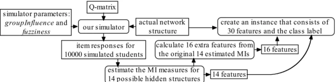
Generating Datasets

Figure 6 shows the main flow of how we create the test records for the simulated students. The simulator requires three different types of input. They include the skeleton of a Bayesian network that