The Mean Estimation of the Combined Quantities by the Asymptotic Minimax Optimization

(1)

AMUEM 2009 - International Workshop on Advanced Methods for Uncertainty Estimation in Measurement Bucharest, Romania, 6-7 July 2009

The Mean Estimation ofthe Combined Quantities by the

Asymptotic Minimax Optimization

Wen-Hui Lo, Member, IEEE and Sin-Homg Chen, Senior Member, IEEE National Chiao Tung University, Taiwan

hs3341.cm90g@nctu.edu.tw, schen@cc.nctu.edu.tw

variables of normal, triangular or rectangular distribution to generate a linearly weighted sum as output, i.e.

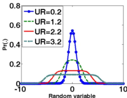
In the basic formulation of the Fotowicz's algorithm, the output of those weighted sums can be approximated by an R*N distribution, which is the convolution of a rectangular function and a normal distribution. The shape of R*N distribution depends on UR known as the uncertainty ratio and expressed by

Abstract-The mean value estimation for the output quantity of combined random variables is one of the major issues in measurement. In this paper, a new quantile-based maximum likelihood estimation (QMLE) method for mean value estimation is proposed. It fuses the concept of both empirical and symmetric quantile to incorporate the order statistics into the QMLE. Unlike Sample mean derived basing only on the maxim um likelihood criterion, the QMLE also considers MMSE defined using the quasi symmetric quantiles (QSQ), i.e., the first- and last-order samples. Simulation results confirm that the proposed QMLE mean estimator outperforms the conventional Sam pIe mean estimator. This work also gives a looking-up table for the refinement corresponding to the QSQ

adjustments. UR:=----;:::::=:::::::::IM=ax=[U=i(x=)]==1

=-~u~

(x) - Max[ui(X)]2

(1)

(2)

(3)

0.2

o

10 Random variable

Fig. 1: Zero mean of R*N distribution for different uncertainty ratio (UR) where K; is a normalization constant. Fig.l displays the R*N pdffor four different values of UR.

0.8rr=========;---.---, ...UR=0.2

0.6 ---UR=1.2 -UR=2.2

f

0.4 -.- UR=3.2

II. PAPER REVIEW

Sample mean is the general usage for the mean value estimation. Its use is convenient because of free pdf assumption for any random variables. If we want to predict the mean value of a combined quantity accurately, the only way is to take Sample mean on heavy observations. The basic where U_i(x) is the standard uncertainty of the i-th input random variable which is of rectangular distribution, and

uc(x) is the combined standard uncertainty. An example of the pdfof R*N distribution is given as

I. INTRODUCTION

In accordance with the Joint Committee for Guides in Metrology (JCGM) Evaluation of measurement data [1], it proposed the concept of quantity expression as a result of propagation of probability distributions. Besides this suggestion, it also considers a generic procedure to determine an estimation for the values of various input quantities which form a hybrid quantity. Up till now, it is convenient and popular to apply the Law of Uncertainty of Propagation to model the standard uncertainty for the combined quantities. But it still lacks a proper formulation to describe the mean value of combined quantities except Sample mean. We would like to cure this weak point via formulating a new mean estimator basing on Sample mean with goal of improving its efficiency.

In our plan, we would like to take the estimator, designed for normal distribution, to estimate the mean value of the output of combined quantities with non-normal pdf Uncertainty can be regarded as a quantization index to measure the performance ofan estimator, hence we introduce the "uncertainty ratio (UR)" as the basic unit to represent the uncertainty. In the formulation of uncertainty for the output of combined quantities, Fotowicz [2, 3] gave a brief description for the case that there is at least one quantity which is submitted to the rectangular distribution. This occurs at a typical occasion of mixing several input random Index Terms-Sample mean, central limit theorem, maximum likelihood estimation, quantile, combined quantities

(2)

Here, the value xp is called the p-quantile of population (or

the output of combined quantities).

volume of requirement for one digit accuracy in measurement is 106 _{observations for 95% coverage interval}

[4]. Sometimes, there are not enough samples to support this rule so that the middle- or small-size sampling plans are also taken frequently. It is known that Sample mean is a uniformly minimum variance unbiased estimator (UMVUE) as well as the random variable of central limit theorem (CLT). Matching to our ideas, we regard Sample mean of the combined quantity as different random variables added together. Bowen [5] has pointed out that CLT may be explained as the sum of independent process whose characteristic function is the product of the component characteristic functions. If we can discard the unbiased requirement, there are still some biased estimators that outperform Sample mean. Stearls [6], and GIeser [7], addressed a new approach for the given coefficients of variation of Sample mean. Ashok et al. [8] further proposed a realistic method to adjust the coefficients of variation of Sample mean to improve its performance.

In this paper, a new method of mean value estimation, referred to as the quantile-based maximum likelihood estimator (QMLE), is proposed. In the single-quantile application, Giorgi and Narduzzi [9] gave a quantile estimation for the self-similar process. Different from the single quantile, our topic focuses on the special style of couple-quantiles, the symmetric quantiles. The classical application of quantiles is the general usage of empirical quantiles, Koenker and Bassett[1 0] extended the empirical quantiles to the regression quantiles, which is especially useful to predict the bounding information. Gilchrist [11] collected many studies about the estimation, validation, and statistical regression with quantile models. Recently, Heathcote, et al. [12] addressed the quantile maximum likelihood estimation ofthe response time distribution. But it involved a time-consuming numerical computation for the inverse of the quantile function, which is typically the cumulative distribution function(cdfJ.

In the proposed QMLE, the quantiles are determined by the maximum percentage of its original population, i.e., coverage. The coverage-constrained quantiles will obey the properties of symmetric quantiles so that the QMLE will be efficient and robust, whose variance asymptotically approaches to the Cramer-Rao lower bound [15]. The symmetric quantiles were described with a strict definition in [15], but we consider them with a more flexible operation to be the ranked variables of the first-order sample xl:_n and the last-order sample x_{n :n •} So, they are both empirical quantiles and quasi-symmetric quantiles (QSQ). We plan to derive the QMLE basing on the order statistics; hence the coverage-constrained quantiles are the endpoints ofthe range. That is, it can support not only the concept of empirical quantiles but also the quasi-symmetric quantiles; otherwise it still needs a quantile function defined below to link quantiles andMLE: (7) (6) 5 Rectangular QSQ 4 Normal QSQ 3 \

-,

\ 2 \_"', "', \ \

_l...

_-

_.

_..

~4 ...-2 0 2

...

~

.

4

(;pn

(n(x -

X

Pn))

r

+

4n(t

(x, -

xpj)

i=l 2n

±~---with the constraint u* > 0 and

x

is Sample mean. where

* C;p:n

(n(x -

xp :n ) )

u==---p 2n

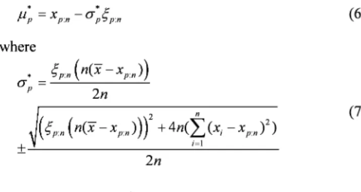
We plot the QSQ of equal variance rectangularpdfas the blue line in Fig.2. It is easily observed that the dispersion of the equal variance ofrectangular QSQ is always less than that of the normal QSQ, while the expectations of theirpdfare close to each other. Huber [13] ever addressed the following robust statistical method via the least possible variance searching and now we plan to take it:

III. THE PROPOSED QUANTILE-BASED MEAN ESTIMATOR

We derive the QMLE by solving the problem of maximizing QMLE(f.1,u) defined by

{

QMLE (P ,O)=

(-~log21l"-nloga)-

t

(x; -

~)2

2 i=l 2u (5)

f.1 == xp :n - UC;p:n· forp ==1 orn

where x_{p :n} is the minimum order (for p=l) or maximum order (for p=n) of samples Xi , 1~i~n ; and C;p:n is a standard normal random variable normalized from x_{p :n ;} and n is the sample size. The solution derived in detail in Appendix is given below:

IV. QMLECONDITIONED ON RELIABLE QUANTILES If we emulate the pdf of combined quantities as a quasi-normal, its extreme shape may be like a rectangularpdf, e.g., the case of UR=3.2 in Fig. 1. As inspecting the distributions of first-order and last-order samples of the rectangular and normal random variables with the same standard uncertainty, we find that the dispersion-areas of QSQ of the rectangularpdfare more concentrated than the normalpdf

Fig. 2: Standard normal pdf combined with its CLT pdf and QSQ pdf for sample size= 11.

(4) Q(p) ==Pr(X

<

xp ) ==p

(3)

0.25

~1 -0.5 0 0.5

We can then apply the minimax operation to Eq.(9) to maximize the objective function.

(9)

!2(Xp :n - flPS)2 2 as 1 {(( * xl:n- flps ) )2 - -₂ X -a· - I I l:n 1 r as

_i

Xi -Xp:n •Xp:n - Jips i=l a as

1(

*

2

*

2)

ArgMax{QMLE(a,flps)-- (fl1 -fl) +(fln-fl) } JLps 2 n 1~ Xi - Xpon 2 = Arg Max{(--log27Z"-nloga)-- L.,( 0 ) JLps 2 2i=l a

D. MMSE criterion applied to the asymptotic minimax optimization

Motivated by the fact that QMLEs are efficient and robust [12], we propose a new QMLE mean estimator incorporating the order statistics for the normal distribution. In accordance with Eq.(9), we realize the optimization ofobjective function in two stages. The first stage takes the roots of differentiation in terms of QMLE, and the second stage takes the QSQ of MMSE under the CLT constraint. By our opinion, QMLE does not guarantee the minimum variance for non-normal data so that we may try the QMLE of normal in association with the MMSE with respect to the QSQ, _{xl:n and xn:n. We} have shown that the QSQ are reliable quantiles in Fig. 2 and its relative formulation as Eq.(9).

~ 0.15

~ CLi

~ 0.1

C. Minimax operations

We define a new objective function via adding an error term to Eq.(5):

0.2

B. Least variance

It is shown in Fig. 3 that the MMSE corresponds to the case that

(f.1

ps -

f.1)

approaches to zero conditioned on heavy

trials. Thus, we may infer to say that the QMLE may probably converge to the population mean for a single trial and is guaranteed to converge to the population mean on heavy trials. Hence, QMLE is near the least variance basing on the MMSE criterion.

(Differences)

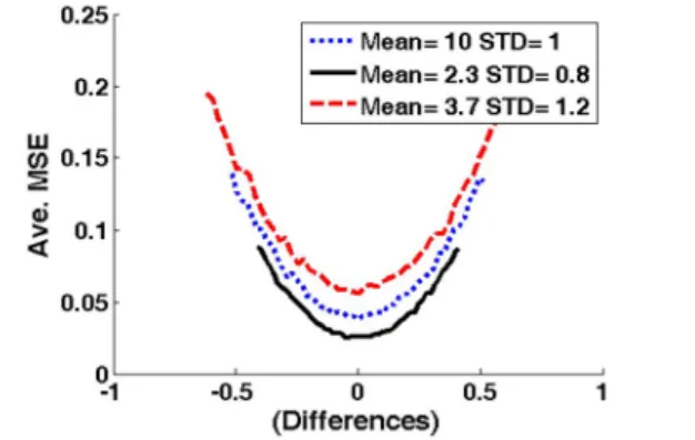
Fig. 3: Average MSE of QMLE versus difference=(flps - fl) for three normal distributions. Note that C;l:n is calculated using true standard deviation a .

0.05

a* is calculated by Eq.(7). We denote it as a;. The final mean estimate is obtained by Eq.(6), i.e.,

u;

=

_{xp:n- a;C;p:n} for p = 1 orn.

We define theMSE for performance measure by

1 1000 ((/-/(i) - fl )2+(fl*(i) - fl )2)

MSE=-L 1 ps n ps (8)

1000 i=l 2

We take the error between the pseudo mean and real mean,

(flps - fl) , as the reference and set the inspection interval of flps to be [fl- 2a /

.j;",

fl+2a /.j;,,], which is the 95% coverage of population mean according to CLT. The inspection interval is determined based on CLT for choosing the best MMSE candidates which only count the two endpoints of range. Remember that the sample variance for the censoring scheme is always smaller than the non-censoring one on heavy data testing. It is thus reasonable to examine the quasi-symmetric quantiles represented by the two endpoints of range, and choose the one with smaller MSE as the best efficient estimator.

We take 50 pseudo means distributed uniformly over the interval. Fig. 3 displays the average MSE of QMLE versus

(f.1

ps -

f.1)

.It can be found from the figure that all the three

curves of average MSE look like convex sets within the CLT searching interval. So, we can conclude that, for all the three test cases using different normal distributions, the average MSEs of QMLE are characterized as convergence curves to become smaller as the absolute value of the difference between flps and fl decreases. Each convergence curve acts

as a convex set.

Asymptotic minimax results: Let K be a convex compact set of distribution F on the real line. To find a sequence T; of estimators of location which have a small asymptotic variance over the whole ofK ;more precisely, the supremum over K of the asymptotic variance should be least possible.

There are three components in the asymptotic minimax result: convex set, minimum variance, and minimax operation. We layout them in details in the following:

A. Convex set

Eq.(5) is a quadratic equation so that there is a global minimum in its curve near the population mean. We use three normal distributions with different mean and variance to demonstrate this assumption. They are N(10,12

) ,

N(2.3,0.82

) and N(3.7,1.22) .In each test, 1,000 trials with

15 samples in each trial are performed. In each trail, the 15 samples are firstly sorted in the ascending order to find the two endpoints, _{x1:n and xn:n. They are then transformed into} the standard normal distributed versions, C;l:n and C;n:n' by

using a pre-assumed pseudo mean

f.1

ps and the true standard

deviation a , or the sample standard deviation

(J"s = ..!.-

i

(Xi -

xl

if(J" is unknown. Then, the estimate n i=l

(4)

QSQ are the wide-sense symmetric quantiles and they have been proved to be more efficient than the regression quantiles [14, 15]. Besides, Chiang et al. [16] suggested to use symmetric quantiles and showed that they are more efficient than the empirical quantiles when the percentage of quantiles is very small or large. Now we denote the two-stage estimator, including applying MMSE-CLT to QSQ for QMLE evaluation, as Q2MMSE-CL T. A sub-optimal searching interval for finding the most possible MMSE candidates can be defined to be uniformly distributed in

Lu -

20-/

.J;z,

f.1+20-/

.J;z].

Here, 0- may be replaced by samples' standard uncertainty o-s ifit is unknown. It is worth to note that the interval covers about 95% coverage of the random variable of Sample mean. It is reasonable to take the MMSE ofthe candidates as the best solution to the combined mean value in the sub-optimal searching interval.

V. EXPERIMENTS ON COMBINED QUANTITIES: Now we evaluate its robustness by simulations using combined quantities formed by input quantities of different pdfs with at least one rectangular pdf We directly test the realistic case that both f.1 and 0- are unknown. Suppose we are given four random quantities as input and they are four independent random variables, including two normal random variables, Zl ---N(0.1,12) and Z2 ---N(2.15,1.52) , and two

rectangular random variables,

Z3 ---rect[

-2.J3

-1.05, 2.J3 -1.05] and Z4 ---rect[-1 0.J3+1.45,10.J3+1.45] .

(10)

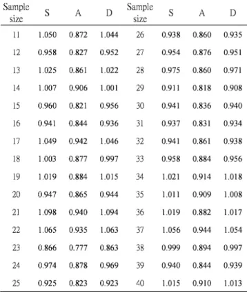
The uncertainty ratio computed according to Eq.(2) is 3.7. Our scope is to test for sample size in the rangeof 11---40. We generate 500,000 samples of the combined quantities and uniformly select the needed observations. We test 5,000 trials for the output of combined quantities for each sample size.

Both Q2MMSE-CL T and Sample mean are estimated in each trial. Table 2 lists the experimental results. Notice that all MSEs are normalize with respect to the square of combined standard uncertainty. After such processing, all the values are in the equal base. There are four conditions encountered in the setting of the searching interval of Q2MMSE-CLT. We list them in the following:

1. Condition A: The CLT searching interval is known and set as [-20- /

.J;z

+u, 20-/

.J;z

+f.1] . The combined standard uncertainty is known as 0-. If Sample mean is larger than 20-/

.J;z

+

u ,

set it as 20-/

.J;z

+f.1 ; and if Sample mean is smaller than -20- /

.J;z

+f.1 , set it as

-20-

/.J;z

+f.1 .

2. Condition B: The CLT searching interval is unknown and set as [-20-

/.J;z

+X,20-

/.J;z

+x] . The combined

standard uncertainty is known as 0- .

3. Condition C: The combined standard uncertainty is unknown. Use the given combined mean and the samples'

standard uncertainty, o-s , to determine the CLT searching interval as [-20-_s

/.J;z

+u,20-_{s /}

.J;z

+f.1] . If Sample mean is out of the searching interval, set it to the bound of the interval, [-20-_s

/.J;z

+u,20-_s

/.J;z

+f.1] . 4. ConditionD:Both the combined standard uncertainty and

combined mean are unknown Set the CLT searching interval as [-20-_s

/.J;z

+

x,

20-_s

/.J;z

+

x] .

TABLE 1: TABLE OF CONFUSION FOR THE CONDITIONS OF COMBINED MEAN AND STANDARD UNCERTAINTY

Population Mean (CLT searching interval) Known Unknown STU of Known A B combined _Unknow quantities _n C D

It can be found from Table 2 that Q2MMSE-CLT significantly outperforms Sample mean for Condition A, and is slightly better for Condition D.

TABLE 2: AVERAGE MSEs RESPECT TO THE SQUARE OF COMBINED STANDARD UNCERTAINTY, 5,000 TRIALS, UNIT IS NORMALIZED TO THE SQUARE OF COMBINED STANDARD UNCERTAINTY, u: (x) / n, S: SAMPLE MEAN, UR=3.7; Sample _S _A _D Sample _S _A _D size size 11 1.050 0.872 1.044 26 0.938 0.860 0.935 12 0.958 0.827 0.952 27 0.954 0.876 0.951 13 1.025 0.861 1.022 28 0.975 0.860 0.971 14 1.007 0.906 1.001 29 0.911 0.818 0.908 15 0.960 0.821 0.956 30 0.941 0.836 0.940 16 0.941 0.844 0.936 31 0.937 0.831 0.934 17 1.049 0.942 1.046 32 0.941 0.861 0.938 18 1.003 0.877 0.997 33 0.958 0.884 0.956 19 1.019 0.884 1.015 34 1.021 0.914 1.018 20 0.947 0.865 0.944 35 1.011 0.909 1.008 21 1.098 0.940 1.094 36 1.019 0.882 1.017 22 1.065 0.935 1.063 37 1.056 0.944 1.054 23 0.866 0.777 0.863 38 0.999 0.894 0.997 24 0.974 0.878 0.969 39 0.940 0.844 0.939 25 0.925 0.823 0.923 40 1.015 0.910 1.013 VI. IMPROVE THE PERFORMANCE BY QSQ ADJUSTMENTS

We have stated earlier that the QSQ expectations of the pseudo-normal pdf are near the QSQ expectations of the

(5)

quasi-normal pdf with the same combined standard uncertainty. Should we adjust the QSQ expectations of the pseudo-normal more closely to the QSQ expectations of the quasi-normal pdf in order to improve the performance of Q2MMSE-CLT? This session discusses the method of improvement and result.

We know that the expectation of coverage IS

(n-1) /(n+1) for different sample size, [17, 18 , 19 ]. According to our standard normal transform, N(0,I2

) , its

corresponding rectangular distribution with equal standard uncertainty is rect[

-.J3,

.J3] . So, the expectation of the first-order sample for the ranked random variable is -.J3+2.J3 /(n+1) . Thus, we may consider adjusting the standard uncertainty of the pseudo-normal pdfto get a better performance. We try to solve the integral equation from the

cdfof normal distribution as:

where a is the adjustment factor multiplying to the original standard uncertainty and we get the following looking-up tables for the value of a depending on the sample size ranging from 11----40:

TABLE3:THE CALI BRATION TABLE FOR SAMPLE SIZE RAGING FROM11~40

Sample _Adjust Sample _Adjust Sample _Adjust

size size size

11 1.46 21 1.12 31 0.99 12 1.40 22 1.10 32 0.98 13 1.35 23 1.08 33 0.97 14 1.31 24 1.07 34 0.96 15 1.27 25 1.05 35 0.96 16 1.24 26 1.04 36 0.95 17 1.21 27 1.03 37 0.94 18 1.18 28 1.02 38 0.93 19 1.16 29 1.01 39 0.93 20 1.14 30 1.00 40 0.92 40 35 -Before C.llb,8tlon - After Callbrdon -.- S8mpleIIlIII!UI - BelateClllbrfltion - After Callbratlon -~

••

~~!~~ - BeforeCalibration

1-

Aft.. C.lbndlon !- S8mple me... 20 30 40 Sample size 20 25 3D 8ample8lze 15 1.4 0.8 0.75 1... 0.9 0.95,...---, ~

!

0.85

~

0.8 ~ 1.1 - -..,---.-- ,-_ _...L....-_----l...._----,I O.8~ Op1O'~"-'-"'15

-,,-,

"'''-20-''---

25--'~'----

3+0"--'---

is

--"-40

Simpleslze &11 1.2

!

1 cj > ~ 0.8 1.2~

~

1t

!

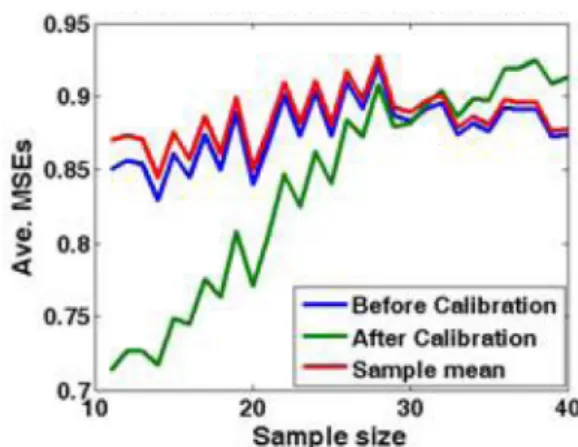
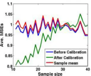
~ OpS, 4

Fig. 4: Prior-Posterior comparison, Condition C, UR=I1.1, 4 combined quantities.

Fig. 6: Prior-Posterior comparison, Condition A, UR=I1.1, 4 combined quantities.

Fig. 5: Prior-Posterior comparison, Condition B, UR=I1.1, 4 combined quantities.

(11)

rf3(~-1) 1 _x2 ₁ ₂

100 n+l --exp(-2)dx~[ - , - ]

00 5a 2a n+I n+I

The testing data are four combined quantities:

Zl ----N(0.1,I2) Z2 ----N(2.15,I.52)

Z3 ----rect[

-2.J3

-1.05, 2.J3 -1.05] and

Z4 ----rect[-

30.J3

+1.45,

30.J3

+1.45] . Fig. -l-Fig. 7 display

the experimental results for the four conditions shown in Table 1. It can be found from Figs.5 and 6 that the refined method works very well for both Condition A and Condition B. We also find from Figs. 4 and 7 that the These figures show that the refined method works well for small sample size, but fails when the sample size is greater than 30.

(6)

1.1,....---..---"""'T"""---, where

Fig. 7: Prior-Posterior comparison, Condition D, UR=I1.1, 4 combined quantities.

VIII. ApPENDIX:

The Quantile-based mean estimator: By substituting

f.1 ==_{xp:n- UC;p:n'} forp ==1 orn , into QMLE(f.1,u) defined in Eq.(5), we obtain

VII. CONCLUSIONS

In this paper, the issue of applying quantile-based maximum likelihood estimation (QMLE) to mean value estimation ofnormal distribution in sparse data condition was addressed. It proposed to incorporate order statistics into QMLE to take the maximum coverage as quantiles so as to conform to the requirement of symmetric quantiles. The asymptotic minimax principle was successfully applied to realize the QMLE mean estimation for combined quantities. The new QMLE estimator combined with the MMSE-CLT to form a new Q2MMSE-CLT algorithm. Simulation results have confirmed that the new Q2MMSE-CLT performs very well to outperform the conventional Sample mean estimator. We showed that the Q2MMSE-CLT earns the greatest gain when the combined mean is known and obtained the least benefit if we take the Sample mean to substitute for population mean in the setting of searching range. The looking-up table only supports the robust estimation on sparse data condition.

REFERENCES

n n

B; ==C;p:n L (Xi - Xp:n) , C; ==L (Xi - Xp:n)2 and u* >0 .

i=l i=l

[1] JCGM, "Evaluation of measurement data -supplement 1 to the guide to the expression of uncertainty in measurement- propagation of distributions using a Monte Carlo method," Joint Committee for Guides in Metrology, final draft, 2006.

[2] P. Fotowicz, "An analytical method for calculating a coverage interval," Metrologia, vol. 43, pp.42-45, 2006

[3] P. Fotowicz, "A method approximation of the coverage factor in calibration," Measurement, vol. 35, pp.251-256, 2004.

[4] ISO, "Guide to the expression of uncertainty in measurement (GUM)-Supplementl: Numerical methods for the propagation of distributions," International Organization for Standardization, 2004, p.12.

[5] B. A. Bowen, "An alternate proof of the central limit theorem for sums of independent processes," Proceedings of the IEEE, vol. 54, iss. 6, pp. 878-879, 1966.

[6] D. T. Searls, "The utilization of a known coefficient of variation in the estimation procedure," Journal of American Statistical Association, vol. 59,pp. 1225-1226,1964.

[7] L. 1. GIeser and1. D. Healy, "Estimating the mean of a normal

distribution with known coefficient of variation," Journal of American Statistical Association, vol. 71, pp, 977-981, 1976

[8] Ashok Sahai, M. Raghunadh and Hydar Ali, "Efficient estimation of normal population mean," Journal of Applied Science, vol. 6, iss. 9, pp. 1966-1968,2006.

[9] G. GIORGI and C. NARDUZZI "Uncertainty of quantile estimates in the measurement of self-similar processes," In: Workshop on Advanced Methods for Uncertainty Estimation Measurements, AMUEM 2008, pp.78-83.

[10] R. Koenker and G.J. Bassett, "Regression quantiles," Econometrica, vol. 46, pp. 33-50, 1978.

[11] W. G. Gilchrist, "Statistical modeling with quantile function," London: Chapman and Hall/CRC, 2002

[12] A. Heathcote, S. Brown, and D.1.K. Mewhort, "Quantile maximum

likelihood estimation of response time distribution," Psychonomic Bulletin and Review, 2002.

[13] Peter1.Huber, "Robustr statistics: a review," Ann. Math. Stat. vol. 43, No.4, pp.l041-1067, 1972.

[14] S.1.Kim, "The metrically trimmed means as a robust estimator of location," Annals of Statistics, vol. 20, pp. 1534-1547., 1992. [15] L.-A. Chen and Y.-C. Chiang, "Symmetric type quantile and trimmed

means for location and linear regression model," Journal of Nonparametric Statistics, vol. 7, pp. 171-185, 1996.

[16] Y.-C. Chiang, L.-A. Chen and H.-C. Peter Yang, "Symmetric quantiles and their applications," Journal of Applied Statistics, vol. 33, iss. 8, pp. 803-817,2006

[17] W.-H. Lo and S.-H. Chen, "The analytical estimator for sparse data," International Association of Engineers (IAENG) Journal of Applied Mathematics, vol. 39, iss. 1,2009, pp. 71-81.

[18] W.-H Lo and S.-H. Chen, "Robust estimation for sparse data," The 19-th international conference on pattern recognition, 2008, pp.I-5. [19] W.-H. Lo and S.-H. Chen, "Theoretical and practical realization for the

uncertainty measurement by coverage interval," IEEE. international instrumentation and measurement technology conference, 2009, pp. 1562-1567 (12) - e.fol. Callb,lllon - After Callbrdon -Semple