ON THE USE OF THE REACH-BACK CHARACTERISTICS METHOD FOR CALCULATION OF DISPERSION

ON THE USE O F THE REACH-BACK CHARACTERISTICS

METHOD FOR CALCULATION OF DISPERSION

JINN-CHUANG YANG AND EUAN-LUNG HSU

Department of Civil Engineering, National Chiao Tung University. Hsinchu, Taiwan 30049, R.O.C.

SUMMARY

The Holly-Preissmann two-point finite difference scheme (HP method) has been popularly used for solving the advection equation. The key idea of this scheme is to solve the dependent variable (i.e. the concentration for the pollutant transport problem) by the method of characteristics with the use of cubic interpolation on the spatial axis. The interpolating polynomials of higher order are constructed by use of the dependent variable and its derivatives at two adjacent grid points. In this paper a new interpolating technique is introduced for incorporation with the Holly-Preissmann two-point method. The new method is denoted herein as the Holly-Preissmann reach-back method (HPRB) and allows the characteristics to project back several time steps beyond the present time level. Through stability analyses it has been observed that the increase of the reach-back time step numbers for the characteristics indeed reduces the numerical damping and dispersive phenomena. A schematic model has been constructed to demonstrate the merits of this new technique for the calculation of the pure advection and dispersion equations. Numerical experiments and comparisons with analytical solutions which support and demonstrate this new technique are presented. KEY WORDS Advection Diffusion Numerical simulation

INTRODUCTION

In predicting the pollutant transport in a one-dimensional channel flow by using numerical simulation, one has to be very careful to avoid the possible diffusion and dispersion induced numerically. Holly and Preissmann' have presented an excellent method for the calculation of advection in one and two dimensions. This method is the well known Holly-Preissmann two- point method (HP method) which is based on the construction of higher-order interpolating polynomials between the dependent variable and its derivatives for two adjacent points on the spatial axis. In comparison with some other existing schemes it has been found that the H P method gives fewest numerical dispersion and diffusion problems. In particular, for the case of transport in a coastal area where the transport phenomenon is dominated by advection rather than diffusion, the numerical damping can be minimized to the greatest extent by using the H P method to compute the advection. Therefore it has been very popular to apply the H P method to solve the mass transport equation.

In fact, the H P method is a kind of characteristics method in which only one characteristic is considered. When one looks at the unsteady flow problems solved by the characteristics method, it is seen that many investigators have improved the characteristics method by including various better and more attractive features: some have extended the characteristics outwards in distance, e.g. References 2-4; others have extended them backwards in time, e.g. References 5 and 6. Each extension has its own appropriate interpolation scheme and its accompanying improvements and

0271-2091/91/030225-11$05.50

0

1991 by John Wiley & Sons, Ltd.

Received October 1989 Revised April 1990

merits. A similar concept of extending the characteristics outwards in space or backwards in time has also been applied to the HP method for solving the advection equation by Yang and Wang’ and Yang and Hsu* respectively. The main aim of the former paper is to extend the original Holly-Preissmann method for solving the dispersion equation under the condition Cr

>

1 (Cr is the Courant number). The latter paper presents a scheme using time line interpolation instead of spatial interpolation for the Holly-Preissmann method.

In this paper a concept similar to the temporal reach-back scheme presented by Laig is applied to the HP method. The key feature of this scheme is that the characteristic is allowed to project back beyond the present time level for spatial interpolation. Error analyses in terms of damping and dispersive factors for the HPRB method are investigated and compared with those for the HP method. In fact, the HP method is a special case of the HPRB method in which no reach-back characteristics are considered. The solutions for the linear advection equation solved by the use of the HPRB method are compared with those solved by the HP method and with the analytical solution.

For the advection4iffusion (i.e. dispersion) problem the split operator algorithm is used to compute the advection and diffusion separately but successively in one time step. For the advection portion, as mentioned previously for the purpose of comparison, both the HPRB and HP methods are used in this paper. For the diffusion portion the well known Crank-Nicholson method is used. A schematic model is constructed to demonstrate and evaluate the applicability of this new technique.

REVIEW O F HP METHOD

For the one-dimensional case the pure advection equation of concentration C of a contaminant can be written as

where x is the distance along the positive direction of flow, t is the time, u(x, t) is the time- dependent flow velocity (assumed to

concentration at any point and time.

along

be directed in the positive x-direction) and C(x, t ) is the Equation (1) can also be stated as

dx

- = u (x, t).

dt (3)

Integration of the above equations yields along

c,=

c,

(4)

( 5 ) X h - X, =

1;

U(X, t) dt.

When u(x, t) = constant = uo,

x h

-

X, = Uo At. ₍₆₎

t 4

n

n - 1

j - 2 j - 1 aAx j. j + l

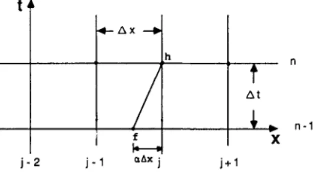
Figure 1. Schematic grid diagram for HP method

concentration for grid point h at time level

n,

which is to be solved. C , is the concentration for grid point

f

at time level n - 1 , in which concentrations for all grid points are known.

Holly and Preissmann' developed a two-point fourth-order method for evaluating ch. They

introduced C,-.', C , and their spatial derivatives C X , - ' , C X , at the present time level as dependent variables to construct a cubic interpolation polynomial over the interval (j- 1 , j):

(7)

where a i d 4 are coefficients which can be found in Holly and Preissmann's paper' and will be restated in the following section;j and j- 1 indicate the computation points; n indicates the time level. The newly introduced variables C X , - and C X , have to be advected also. By following a similar procedure to that described above,

cxh

can be obtained as

(8) where b,-b, are coefficients which can again be found in Holly and Preissmann's paper' and will be restated in the following section also.

Ch =

cf

= a1

c;::

+

a2 C ; - l + a3 C x y : :

+

a4CXy'

'

CXh= c X , = bl C y I :

+

b,Cj"-'+ b 3 C X ; I :

+

b,CX;-',

DESCRIPTION O F NEW METHOD

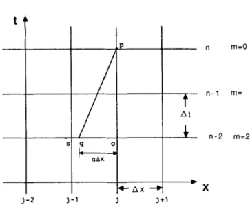
As mentioned previously, when the concentrations are known only at fixed grid points, referring to Figure 1, interpolation is usually required to calculate the unknown concentration for the characteristics. Instead of the HP spatial interpolation technique described previously, the present method is to let the characteristics project back beyond the present time level for the spatial interpolation as indicated in Figure 2. The similar interpolating function can be expressed as

C,= C q = a l CQn-"

+

a2Cz-" +a3 CX:-"+ a,CX:-", ₍₉₎

where C"-" and CX"-" denote the concentration and its derivative with respect to space at time level n

-

m as indicated in Figure 2; m is the reach-back number; s and o represent any two adjacent points which the characteristics foot on the spatial axis falls in between. The coefficients ~ 1 - ~ 4 are expressed as

a,=a2(3-Za), a 2 = 1 - a l , a,=a2(1-a)Ax, a4= -a(l-a)2Ax,

where a is the interpolation parameter which is the decimal portion of mCr and is self-explanatory from Figure 2; Cr is the Courant number. A similar argument to that for deriving equation (8) has also to be taken into account here. The derivative of concentration also has to be advected.

t 4

n n - 1 n - 2 m=O m= m=2 X j -2 j - 1 j j +1

Figure 2. Schematic grid diagram for HPRB method

Therefore C X at point p can be obtained as

C X , = C X , = b , C:-"'+ b Z C : - m

+

b , CX:-"+ b4CX!-"',

where

b , = 6a(a

-

l)/Ax, b , = - b ,

,

b,

= a(3a - 2), b4 = (a

-

1) (3a

-

1).

Equations (9) and (10) complete the calculation of pure advection of the concentration and its derivative for one time step. This scheme is of fourth-order accuracy. The coefficients a1-u4 and

b,-b, are identical to those of the original Holly-Preissmann method and are unchanged by the process of allowing the characteristics to project back beyond one time step.

ERROR ANALYSIS

The accuracy of the scheme can be investigated through the analysis of the errors in the calculation of pure advection of a simple sine wave. An error analysis is performed to provide quantitative information by using the von Neumann method," which assumes the solution can be described as a linear sinusoidal wave.

The error analysis results in two quantities, the damping factor R, and the wave speed factor R,. R, is the modulus of the complex ratio of numerical solution to actual solution after one time step. R, is the ratio of numerical wave speed to actual wave speed after one physical wave travel time.

From the advection equation (1) a Fourier series solution is assumed. When it is written for the grid points the solution can be expressed as

m

k = 1

~ ( X Y t)'

1

Ckexp[i(akx+pkt)]~ (1 1)

where a = 2n/L ( L is the wavelength) and

p

= 2a/T ( T is the wave period). By focusing on the kth term and substituting into equations (9) and (10) one can obtain the relations

Ck(exp(i/3krnAt)-a,exp[-iak(r+ l)Ax] -a,exp(-ira,Ax)}

CX,(exp(i/?,rnAt)-b,exp[ -io,(r+ l)Ax] -b4exp( -iro,Ax)}

+ C k { -b,exp[-i(r+ l)a,Ax]-b,exp(-ira,Ax))=O, (13) where r is the integer portion of mCr, At is the time interval and

Ax

is the space interval. The eigenvalues are determined by setting the coefficient determinant to zero. By letting

cp = exp(i&At) and

6

= exp(

-

io,Ax), one can obtain

The complex amplification factor cp, which can be solved from the above equation, provides insight to the stability and numerical dispersive character of the numerical scheme; cp can also be expressed as

cp = ~ ( C O S 8

+

i sin 0), _{(1 5 )}

where is the amplitude of cp and O is the degree of cp. Then the amplification factor R , and the dispersive factor R , for one time step can be obtained as

where I = L/Ax.

Figures 3(ab3(e) show the amplitude portraits for Cr =01,0*25,0*5,0.75 and 0.9 respectively. Each figure shows a comparison of the results for reach-back numbers m = 1,2,3 and 4. In fact, the case for m = 1 is identical to the HP method. From all of these figures one can deduce a general tendency, namely the values of R , and R , approach unity when no damping occurs as the reach- back number m increases. For Cr = 0.25 (Figure 3(b)) the value of R , for m = 4 is equal to unity; this is so because the characteristic intercepts the grid point at time level m = 4. Similarly, for Cr =0.5

(Figure 3(c)) one can observe that R, = 1-0 when m =

2

and 4; and for Cr =0*75, R , is equal to unity when m=4 as shown in Figure 3(d). This should also be true for the phase portraits shown in Figures 4(a)-4(d). In particular, it is known that for Cr = O m 5 the value of R , will always be equal to unity for any value of m. Therefore the phase portrait for Cr=0.5 is not shown here.

In addition, Figures 3(a)-3(e) indicate that the resolution for R, increases as the reach-back number increases. Similarly, Figures 4(a)-4(d) show this consistent tendency for the phase portraits. If this is the case, then it becomes very important for one to determine how large a reach- back number should be used. From several test cases and the results discussed above it seems that the reach-back number m = 4 should be sufficient. Using a larger value of reach-back number gives an insignificant improvement in resolution. In addition, difficulties in setting up the initial conditions may arise when a large reach-back number is used.

SOLUTION FOR DISPERSION EQUATION

The linear dispersion equation can be expressed as a combination of pure advection and diffusion. The equation can be written as

DC

azc

dx

-=v- along

d t = ~ O ,

Dt

ax,

0.89 ~ 0.88 ~ 0.87

(4

1 .oo 0.99 0.98 0 97 0 96 0.95

-

0.94 n 0.93 n 093 - 0 9 2 - 0 9 1 - 0 9 0 - 089 - 0 8 8 - 087

:;;

Ica,,

, , , , ~ , , , , 0.89 0.88 0.87 2 3 4 5 6 7 8 9 10 1 1 12 - 13 1: L/DX (el , , , , , , , , , , , , , , , , 0.98 0.97 0.96 0.92 0.91 0 90 0.89 0.88 I I , , , I , , , , 8 9 10 1 1 12 13 14 15 16 17 1's lb L/DX 1 .oo 0 99 0 98 0.97 0 96 0.95 0.94 0 93 0.92 0.91 0.90 0.89 0.88 0 87 M exo

-

m=1 _d m = 2

-

m=3 ctseful m = 4 LY L/DX 100 0.99 0.98 0.97 0 96 0.95 w

-

e m m=l -+a m=2

-

m=3 oeess m=4

0.96 - 0.94 - 0.92 - 0.90 - 0.86

:::

1.04 (b) [L 0.98 - 1.0004 - : - I I -A exa m = l N o m=2 t m=3 a m=4 [r 0.9994

-

:"',

, , , , , , , , , , , , , , , 0.90 0.88 0.86 4 5 6 7 8 9 10 1 1 12 13 14 15 16 17 18 19 L/DX ( 4 0.9992 1.08

4

0.99970

-

0.99965

-

1.04 ' . 0 6

h

(4 1 .wow 0.99995 0.99990

y

I

0.99985

2

0,99980 0.99975 A exo m=1 o m = 2 m=3 8 m=4

This equation can be solved

by

decomposition into pure advection and pure diffusion using a split operator method.' The advection can first be solved

by

the HPRB method as described in the previous section. The concentration and its derivative after the advection are denoted as C; and

C X ; . Then the diffusion portion can be computed by use of the Crank-Nicholson method, which can be expressed as (1 - $)vAt

(c;;;-2c;-1+c;I;),

$vAt Ax2 Ax2

c;

-

c; =--c;+

1

-

2ci"

+

c;-

+

By the same argument as that stated in the advection portion, one has to diffuse the term C X . The expression for the diffusion of C X can be written as

*vAt ( l - + ) v A t

cx;-cxja=-(cx;+l

- 2 c x ; + c x ; - , ) +

(cx;;:

- 2 c x ; - ’ + c x ; 3 . (20)

Ax2 Ax2

From equations (19) and (20) the concentration C and its derivative C X after the diffusion process at the next time step t” can be obtained. This completes the calculation for the dispersion equation.

DEMONSTRATION AND EVALUATION

Calculation of pure advection

The pure advection of a Gaussian concentration distribution for different velocities, i.e. for different Courant numbers Cr, with constant At and Ax, has been computed. The distribution of mean position 3000 m and standard deviation 200 m is defined on the regular grid Ax = 200 m.

Upstream and downstream boundary conditions are assumed to be C = 0 and C X = 0 respectively. Test cases with Cr = 0.1,0.25,0.5 and 0-9 are simulated for time t = 7oooO,28000,14000 and 8000 s

respectively. When a reach-back number m greater than unity is used, other schemes may be

i

n

1

-

-

-i\

10 9 8 )).ex0 7

-

m=1

-

rn-2

-

m=3

-

nl=4 $ 6 Q. E 5 8 4 8 5 2 1 0 1 -1

‘

Bwo LIMD o m 95M) l r n 10500 1 1 m l l M O 12ooo 8000 8500 9000 9500 lWo0 10500 1lWo 11500 12000

DISTANCE (m) DISTANCE (m) 10 8g

;[

342 1 0 10 9 8 7 6 6 $ 5 I g 4 8 3 2 1 0

needed to set up the initial conditions. For those cases studied herein the H P method is used to establish the initial condition.

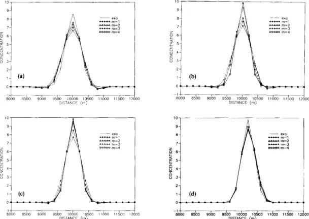
The results computed by the use of HPRB with various reach-back numbers and the analytical solution are shown in Figures 5(ab5(d). In fact, when rn= 1 the HPRB method is identical to the original H P method. From Figure 5(b) it can be seen that the solution for Cr =0.25 and m = 4 is identical to the analytical solution. This situation was explained previously because the characteristic falls exactly on the grid point, hence no error exists. The same situation can be found in Figure 5(c) for Cr = 0.5 when rn = 2 and 4. From these test simulations it can be concluded that the results get better, i.e. closer to the exact solution, as the reach-back number rn increases. However, when the characteristic closes to the grid point, such as is the case for Cr=0.9 (Figure 5(d)), the effect due to the increase of rn will not be so significant. This should be obvious since the exact solution will be obtained when the characteristic falls on the grid point.

Calculation of dispersion

A Gaussian distribution and the same boundary conditions as mentioned previously are used for the calculation of the dispersion. Cases with Cr = 0.1, 0*25,05 and 0-9 are studied for reach- back numbers rn= 1,2, 3 and 4. The diffusivity used for these studies is 0.1 m2 s-'. The results for all of the test cases are shown in Figures 6(abqd). From these results it can again be seen that an

- e m

-

m=1 _d m=2 m=3 _(I m=4 - exa

-

m=1 _d m=2

-

m=3 _(I m=4 & - 1 4 - r v - - - , - T 1 -8000 8500 9000 9500 10000 10500 Il000 11500 1: DISTANCE (m) DISTANCE (m) 9 8 7

-

m=1

-

m=2

-

m=3 5 6 g 5 $ 4 8 3 2 1 0

I

_{- i o b} 9 o b o - l o d o O lOJ00 11doo 11400 l i DISTANCE (m)

&k&

s o b o h 0 x O & x 11500 12000 DI5IANCE ( m )

Figure 6. Comparison of analytical solution and numerical solution for dispersion equation: (a) Cr=O.l, t=70000s;

(b) Cr = 0.25, t = 28OOO s; (c) C r = 0 5 , t = 1 4 0 0 0 s ;

(d) Cr=0.9, t=SOOOs

increase in reach-back number gives better results, but again the improvement will not be obvious when the characteristic approaches the grid point, such as is the case Cr = 0.9 (Figure qd)).

CONCLUSIONS

The Holly-Preissmann two-point fourth-order scheme has been a very popular and successful scheme for computation of the advection equation. On the basis of the main framework of the H P method, in this paper a new interpolation technique taking into account the reach-back characteristics is introduced. From the stability analysis and the demonstration of the test simulation, one finds that for the advection problem an increase in reach-back number can reduce the numerical diffusion and dispersion problems. When the characteristic projects back exactly on the grid point, the result computed is identical to the exact solution. The dispersion equation is solved by the split operator algorithm. The advection portion is calculated by using the HPRB scheme and the diffusion portion is computed by using the Crank-Nicholson scheme. For the weak diffusion case presented in this paper, the effect due to the increase of the reach-back number is quite convincing. Furthermore, on the basis of the numerical experiments and the demon- stration presented, the reach-back number m = 4 seems to be sufficient for accurate calculation. In

practice, the higher the reach-back number used, the better are the results that can be obtained. The use of m = 4 is a compromise which already gives a significant improvement in solution accuracy without introducing problems in initiating the calculation.

ACKNOWLEDGEMENTS Lee. a 1Ca4 b 1 4 4 C

cx

I

j

k

L m n R l R2 T t U X Ax At V c7

The authors would like to express their appreciation for the funding support from the National Science Council of Taiwan and for the assistance in the drawing preparation by Mr. Jen-Chung

APPENDIX: NOTATION coefficients for the interpolation polynomials coefficients for the interpolation polynomials concentration

concentration derivative with respect to space dimensionless spatial discretization, L/Ax computation point

component of sinusoidal wave length of sinusoidal wave

integer denoting reach-back number time level index

damping factor dispersive factor wave period time velocity

distance along the flow direction space increment

time increment diffusivi t y

B

2n/T

4

exp(iak Ax)

i

amplitude of cp 8 degree of cp

*

weighting factor cp exp(iBkAt) REFERENCES

1. F. M. Holly Jr. and A. Preissmann, ‘Accurate calculation of transport in two dimensions’, J. Hydraul. Diu. ASCE, 98.

1259-1277( 1977).

2. F. F. M. Chang and D. L. Richards, ‘Deposition of sediment in transient flow’, J . Hydraul. Diu. ASCE, 97, 837-849

(1971).

Conf: on Pressure Surges, BHRA, Fluid Engineering, Cranfield, 1977, pp. 15-30.

3. A. E. Vardy, ‘On the use of the method of characteristics for the solution of unsteady flows in networks’, Proc. 2ndInr.

4. D. C. Wiggert and M. J. Sundquist, ‘Fixed-grid characteristics for pipeline transients’, J . Hydraul. Diu., ASCE, 103, 5. E. B. Wylie, ‘Inaccuracies in the characteristics method’, Proc. 28rh Ann. Hydraulic Specialty Con$ ASCE, Chicago, IL, 6. D. E. Goldberg and E. B. Wylie, ‘Characteristics method using time-line interpolations’, J. Hydruul. Eng., ASCE, 109,

7. J. C. Yang and J. Y. Wang, ‘Numerical solution of dispersion equation in one dimension’, J . Chin. Inst. Eng., 11,

8. J. C. Yang and E. L. Hsu, ‘A new technique for numerical solution of dispersion equation’, J. Hydraul. Res., I A H R ,

9. C. Lai, ‘Comprehensive method ofcharacteristics models for flow simulation’, J. Hydraui. Eng., A X E , 114, 1074-1097

1403-1416 (1977). 1980, pp. 165-176. 67-83 (1983). 379-383 (1988). 28(4), in press. (1 9881.

10. J. Von Neumann and R. D. Richtmyer, ‘A method for the numerical calculations of hydrodynamic shocks’, J. Appl.