STUDY OF ACOUSTIC-RESONANCE IN ENCLOSURES USING EIGENANALYSIS BASED ON BOUNDARY ELEMENT METHODS

Study of acoustic resonance in enclosures using eigenanalysis based

on boundary element methods

Mingsian R. Bai

Department of Mechanical Engineering, National Chaio Tung University, 1001 Ta Hsueh Road, Hsin Chu 30050, Taiwan, Republic of China

(Received 17 August 1991; accepted for publication 6 February 1992)

It is well known that, from the modal theory of room acoustics, resonance will occur if the driving frequency of a sound source located in a room coincides with one of the natural frequencies of the sound field. In this study, an eigenanalysis technique based on the boundary element method (BEM) is developed for extracting eigenmodes of a sound field in an

enclosure. A method of singular value search, in conjunction with a golden section

optimization algorithm, is utilized for efficient calculation of eigenmodes. In particular, modes associated with repeated eigenvalues can be well resolved by the technique developed in this research. Enclosures of various geometries have been analyzed by using the developed algorithm in a numerical simulation. Satisfactory agreement has been achieved between the BEM results, the FEM results, and the analytical solutions if available.

PACS numbers: 43.20.Ks, 43.55.Br

INTRODUCTION

Resonance phenomenon in an enclosure is one of the

important subjects in research of acoustics. The importance

lies in the fact that the knowledge of acoustic eigenmodes is essential to the analysis of dynamic responses of a sound field

in an enclosure. For example, modal theory is employed in

room acoustics for analyzing reverberation phenomena

when ray acoustics does not provide, especially for low and

intermediate frequency ranges, a complete modeling of

sound

fields

in an enclosure.

1.2

Adequate

distribution

of res-

phenomenon of combustion chambers. Research 3 has

shown that combustion knock, which is harmful to engines,

is mainly due to acoustic resonance in combustion cham-

bers. Proper tuning of resonance frequencies will reduce combustion knock to a minimum so that engine perfor- mance can be improved.

While separable coordinate systems 4 are available for

analytically calculating acoustic eigenmodes in dealing with enclosures of simple geometries, one has to resort to numeri- cal methods, e.g., the finite element method (FEM) and the

boundary element method (BEM) for enclosures of com-

plex geometries. Since only boundary meshes need be con- structed in the application of BEM, dimensionality of the original problem is reduced by one. This fact makes BEM a particularly attractive technique for eigenanalysis of enclo-

sure resonance.

The objective of this study is to develop a numerical technique for extracting acoustic eigenmodes in enclosures based on the boundary element formulation and to demon- strate how best to implement it. Problems involved in the implementation phase including resolution of eigenmodes associated with repeated eigenvalues and algorithms of effi- cient search for eigenmodes are investigated. In order to ver- ify the BEM-based eigenanalysis technique, a rectangular room with a known exact solution is selected as the first test

object in a numerical simulation. Numerical performance of the developed method is also compared with that of another commonly used method, FEM. Higher accuracy has been achieved by using BEM than FEM. Then, both methods are applied to the case of a car interior. The results of eigen- modes obtained from these eigenanalysis methods display excellent agreement.

I. THE BEM-BASED EIGENANALYSIS TECHNIQUE

In the beginning of this section, the theory of integral equations for the boundary value problems of sound fields will be briefly reviewed. Then, a BEM-based eigenanalysis technique in conjunction with eigenmode search schemes will be presented. Some technical problems during the im- plementation phase will also be discussed.

A. The BEM-based eigenanalysis of sound field in an enclosure

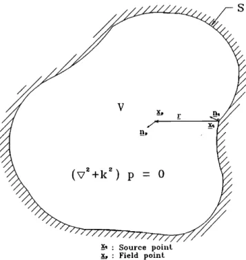
From the theory of linear acoustics, it is well known that

the solution of a boundary value problem (see Fig. 1 ) asso- ciated with a monochromatic sound field in an enclosure is represented by the following Kirchhoff-Helmholtz equa-

tion: *-6 where

ap(xp

) = G(xp,Xq

) • (Xq)

-- p(Xq

) • (Xp,Xq)dSq,

x•S,

S a smooth

surface

x•S, S a nonsmooth

surface

(11 is the solid angle). 5

(1)

••/• (va+k•)

P

= 0

x_• ß Source l)oint

xp. Field point

FIG. 1. Schematic diagram for the interior boundary value problem of a

sound field in an enclosure.

sured at the location x. The free-space Green's function

G(xp,Xq

) = exp(ikr)/4rcr

for the Helmholtz

equation

in a

ing the speed of sound). The position vector xp and Xq de-

note, respectively, the field point and the source point. The

distance

r = Ix• -- xql. The directional

directive

8/Sn =n-V

On the basis of boundary integral equations, we are now in a position to develop a BEM-based technique for the ei- genanalysis of a sound field in an enclosure. In this study, triangular elements and quadrilateral elements are used to construct a mesh on a surface. Isoparametric transformation is adopted for discretizing a boundary. The same set of qua- dratic shape functions are used to interpolate global coordi- nates, sound pressures, and pressure gradients on a bound-

ary as follows: 7 L

Xi (g) = Z N/(g)x,, i = 1,2,3;

L = 6 or 8,

(2)

Pro(g)= • Nt(g)pm•, m=l,2,...,M; L=6 or 8, (3)

8%

(g)

= • N,(g) , m=

l= 1

•nq

1,2,...,M;

L=6 or

8,

where x, is the ith coordinate of the l th node, N• (•) are the quadratic shape functions, •----(• ,•2 ) are the local coordi-

nates,

pro/and

t•pmt/t•rt

q are the sound

pressure

and

the pres-

•nq

into Eq. ( 1 ) gives the following discretized boundary inte- gral equation:

aip(xp)

m=l

(5)

where

a• is the solid

angle

parameter

of the field

point

x v, VG

(•,) m are L X 1 column vectors corresponding, respective-

ly, to Pm•

and •m•/•nq terms

in the integral

equations,

and

N (g) is an 1 X L row vector with N• (g) as its components.

In terms of operator notation, Eq. (5) can be assembled into the following matrix form for a mesh with M elements and N

nodes on the boundary:

ai•(Xp) = sPq•g

-- wq• q,

(6)

sound pressure

p(Xq) and the pressure gradient

•p (Xq)/•nq, respectively,

of the N nodes

Xq,

and

S vq

and

wq

the spatial

transformation

from the field point x v to the

source points Xq.

Now, taking the field points to the boundary S and set-

ting a• = i or •/4v (• denotes

the solid

angie

at the field

point

x v and i = 1,2

.... ,N), depending

on whether

the sur-

face is smooth or not, one obtains

•q = sqq•g -- Dqq• q (7)

or

Dp q = Sqqpg, ( 8 )

where a is an N X N diagonal matfix whose diagonal terms are composed of the parameters a i's corresponding to the N nodes on the boundary. D qq and S qq are both N X N square matrices corresponding to the integrals in Eq. (5) relating

the N field points

x v and the N source

points

Xq on the

and D • (D qq + a).

In some situations, care should be taken for the treat-

ment of nonsmooth surfaces. Recall that the parameter a• in

•. (5) equals

• for smooth

surfaces

and •/4w for nons-

ed by applying a uniform potential to the inte•or domain to yield 7

= - fs

W(x,Xq

(g))-nq

(g)IJIN

dSq

]qu

or

Oti

= -- E (Dqq)o'

(9)

j=l

u denotes an N X 1 column vector whose terms are all ones, and (D qq) ii are the components of D qq.

In this study, the walls of enclosures are assumed to be rigid, which is approximately true in many cases, e.g., a hard-walled room. This corresponds to imposing the bound- ary condition •3p/•3n = 0 on $. Thus, Eq. (8) is simply re- duced into

Dp = 0. (10)

Here, Eq. (10) constitutes the main equation of the BEM- based eigenanalysis of a sound field in an enclosure. In prin- ciple, the wave numbers k's that render the matrix D singu- lar should be the desired eigenvalues. The eigenvectors associated with each eigenvalue can be obtained from find- ing the nontrivial solutions of Eq. (10). Nevertheless, care should be taken because Eq. (10) is not the usual form of the generalized eigenvalue problem Ax = )[ Bx and accordingly must be handled differently. In the case of the BEM-based formulation discussed herein, the eigenvalues are embedded

in the kernel functions G or o•G/o•n and the coefficient matrix

D is a function of the eigenparameter A. This peculiarity of the BEM-based formulation precludes the use of standard eigensystem solvers such as those widely used in the FEM. Therefore, special eigenmodes search schemes, e.g., the method of determinant search and the method of singular value search, are developed in this study to alleviate this numerical difficulty.

B. The search schemes for eigenmodes

In the method of determinant search, one seeks to deter- mine the eigenvalues by incrementally varying the wave number k such that the matrix D in Eq. (10) becomes singu-

lar.

8'9 This amounts

to finding the wave numbers

k e,

e -- 1,2,..., so that the determinant of D vanishes. In numeri-

cal implementation, however, one can only search local minima of the determinant of D for the eigenvalues because it is virtually impossible for D to become ideally singular

except for some special cases. •ø Once the eigenvalue ke's

have been found, the natural frequency co e's can readily be recovered from W e = k ec.

In addition to eigenvalues ke's, the eigenvectors pe's re- main to be found. The eigenvector Pe, which represents the eigenmode associated with the eigenvalue co e, is, by defini- tion, the nontrivial solution of the following equation:

DePe --0, (11)

where the N X N matrix De is obtained from the coefficient matrix D evaluated at k = ke and the eigenvector Pe is an N X 1 column vector. These nontrivial solutions of Eq. ( 11 ) can be calculated by the Gauss elimination algorithm.

In addition to the previously mentioned determinant search method, another approach based on singular value decomposition (SYD) is developed in this study for calcu-

lating eigenmodes. From the theory of linear algebra, the

following decomposition of an arbitrary matrix D is always

possible: 11

D = UI•V h, (12)

where h is the Hermitian conjugate operator, U and V are

both N X Nunitary matrices and are composed of Northogo- nal column vectors ui's and vi's, respectively, and •; is a pseudodiagonal matrix (but is a diagonal matrix in our

case)'

0'i

•0, i--j

Z/•=

O, i•:j

(rri's are singular values arranged in descending order). If the matrix D is almost singular, then the rank of D tends to be degenerate with the last one or more singular values being nearly negligible in comparison with the rest of singular val- ues. In the initial stage of extracting the eigenvalues ke's, the coefficient matrix D is evaluated with the wave number k incrementally varied by a coarse step size Ak. In each iter- ation, the matrix D associated with different k is processed by the SVD algorithm. The minimal singular value obtained

at the rth iteration (denoted by rr•,r ) is compared with the

minimal singular values fry's obtained from the other itera-

tions. If rr•,r is smaller than those obtained from the adjacent iterations, i.e., rr•.•_ • and rr•,• + •, then at least one eigenval- ue must exist within the interval (k- Ak, k + Ak).

Having established a search interval for an eigenmode, one may proceed to calculate a more accurate value of a particular mode. Instead of using a sequential search proce- dure, a more efficient optimization technique termed the

"golden section search algorithm "•2 is then utilized for lo-

cating the eigenvalue of interest. This simple search method is selected because the gradient of the cost function (which is

difficult to estimate in our case) is not required. In general it

takes less than 10 search step to reach accuracy within two decimal places.

Parallel to searching for eigenvalues, the eigenvectors are obtained from the SVD process without additional ef- fort. This is manifested by postmultiplying Eq. (12) by

(vh) -•.

•(V h) -• =

or

DV = U• ( 13 )

since vh= V-1 from the property of unitary matrices.

Further partitioning of Eq. (13) yields

D¾ i = O'ill i. (14)

Whenever the singular value o' i • 0, Eq. (14) becomes

Dvi = 0. (15)

Direct comparison of Eqs. (10) and (15) reveals that the eigenvector ¾i in the latter equation is a legitimate nontrivial

solution of Dp = 0. In other words, whenever cr• vanishes,

the right singular vector vi of D can be regarded as an eigen-

vector associated with the eigenvalue k,.

In addition, this SVD approach for finding eigenvectors

is particularly useful when the eigenvalue problem of con-

cern involves nondegenerate repeated eigenvalues (which

are frequently encountered in the cases of enclosures with high degree of symmetry). For instance, if the eigenvalue k, is of multiplicity m, then the last m singular values

an -- rn

+ 1 ,an -- rn

+ 2 ,"-,an will be significantly

smaller

than

are accordingly the desired linearly independent eigenmodes associated with the same eigenvalue ke. In this regard, the method of singular value search has more preferable perfor- mance than the method of determinant search because the latter approach fails to provide linearly independent eigen- vectors for the cases involving repeated eigenvalues. Thus, in the following sections, the method of singular value search is

selected in the BEM-based eigenanalysis for calculating

eigenmodes of sound field in an enclosure. II. VERIFICATION OF THE BEM-BASED EIGENANALYSIS ALGORITHM

In order to investigate numerical characteristics of the developed BEM-based eigenanalysis technique, computer simulations are conducted for extracting eigenmodes of a sound field in an enclosure. The BEM result is compared with the corresponding analytical solution. For a case where the analytical solutions is not available, FEM is selected as an alternative numerical approach. The formulation of the FEM-based eigenanalysis is omitted here because it is quite

standard and can be found in the literture. 13-•6

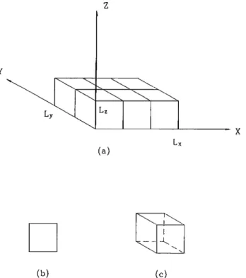
The first simulation case involves determination of eigenmodes of a rectangular room. Consider a rectangular

room bounded by rigid walls lying along the planes x -0,

x -- L,,, y = O, y -- Ly, z = O, z -- Lz, as shown in Fig. 2 (a).

The boundary value problem can be expressed in terms of rectangular coordinates as

82P

+ 82P

+ 82P

+k2p-O

(16)

09x 2 09y2 09F

subject to 8p/Sn = 0 on the walls. It can be shown4 that the

Lx

(b) (o)

FIG. 2. (a) The mesh for the rectangular room used in the numerical simu- lation. (b) The boundary element used in the mesh. (c) The finite element

used in the mesh.

eigenvalues of the above boundary value problem are

+

with the associated eigenfunctions

p (x,rt • ,fly ,rt z ) = ,4 COS • /•/x 7TX COS /•/y 7Ty COS • /•/z 7TZ

L,, Ly Lz

(18)

where A is an arbitrary constant. Here, an eigenmode is iden-

tified by a particular combination of integers n,,, ny, and he.

Each of these three integers is assumed nonnegative to avoid redundancy. In this simulation, a rectangular room bounded

by rigid walls of dimensions Lx- 3 m, Ly- 2 m, and

Lz -- 1 m is selected for testing the BEM-based eigenanalysis algorithm.

The results obtained from the BEM-based algorithm are first compared with the corresponding analytical solutions to check if the algorithm is correctly implemented. Since the BEM used for eigenanalysis purpose is a relatively new ap- proach, it is worthwhile to compare its numerical perfor-

mance with the other methods. To this end, the BEM-based

approach is compared with another commonly used numeri- cal method FEM in this simulation. The mesh of BEM co- alesce with that of FEM on the boundary in order to achieve

a fair comparison. In this case, 22 quadratic rectangular ele-

ments with 68 colocation points are used for constructing the BEM mesh, while 6 quadratic brick elements with 70 colocation points are used for constructing the FEM mesh (Fig. 2).

The minimal singular values tr n's are computed by vir- tue of the SVD algorithm for different wave numbers k's with initially a coarse step size Ak (0.1 in this case), as shown in Fig. 3. Whenever a local minimum occurs, its adja- cent wave numbers are chosen as a search interval for the golden section search algorithm that gives more accurate eigenvalues. In addition to the BEM-based approach, the same case of a rectangular room is analyzed by FEM. The results obtained from both numerical methods are then com-

Minimum singular value

0.08 0.06 o.o,i 0.02 o o o.5 i l ..5 3 Wave number

FIG. 3. The minimum singular values •r.'s calculated for each wave number k in the case of a rectangular room.

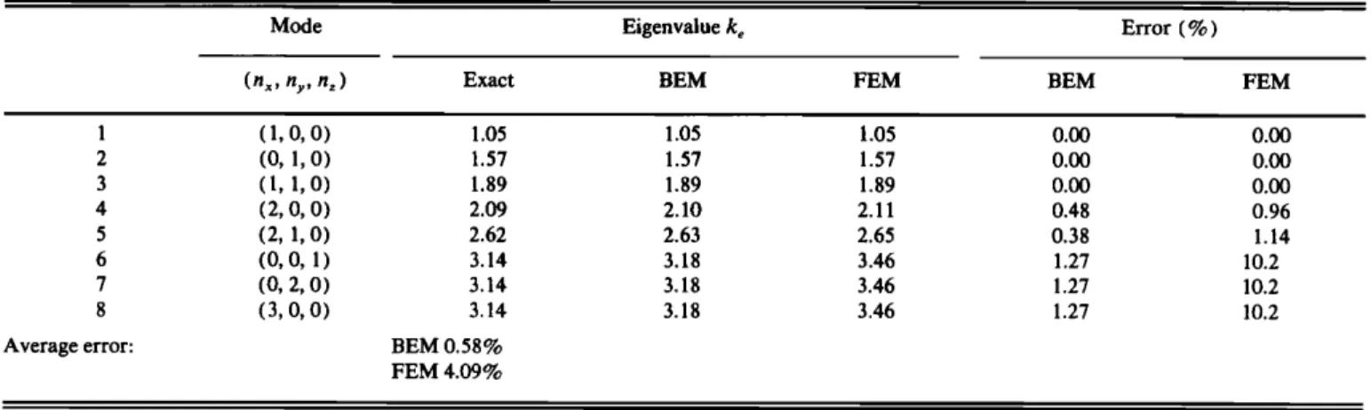
TABLE I. Comparison of eigenvalues of the sound field in a rectangular room.

Mode Eigenvalue k e Error (%)

(nx, %, nz ) Exact BEM FEM BEM FEM

1 (1, 0, 0) 1.05 1.05 2 (0, 1, 0) 1.57 1.57 3 ( 1, 1, 0) 1.89 1.89 4 (2, 0, 0) 2.09 2.10 5 (2, 1, 0) 2.62 2.63 6 (0, 0, 1) 3.14 3.18 7 (0, 2, 0) 3.14 3.18 8 (3, 0, 0) 3.14 3.18

Average error: BEM 0.58%

FEM 4.09% 1.05 0.00 0.00 1.57 0.00 0.00 1.89 0.00 0.00 2.11 0.48 0.96 2.65 0.38 1.14 3.46 1.27 10.2 3.46 1.27 10.2 3.46 1.27 10.2

pared with the corresponding analytical solutions in Table I. A sharp contrast of numerical performance is immediately observed from the table. The BEM achieves much higher accuracy (with an average error ofeigenvalues 0.58% ) than the FEM (with an average error of eigenvalues 4.09%). This could be attributed to the fact that the integral formula- tion of BEM has well-posed numerical characteristics in comparison with the weak formulation of FEM. Neverthe-

less, the higher the mode, the larger the error is, regardless of

which method is used. In any event, to what extent one is able to search for eigenvalues is basically limited by sound wave length in comparison with the mesh spacing.

Another interesting observation worth mentioning is as-

sociated with the last three modes (0, 0, 1 ), (0, 2, 0), and ( 3, 0, 0) listed in Table I. These modes correspond to the same eigenvalue 3.14 and are successfully detected by the method of singular value search. The last three singular values com- puted from decomposing the coefficient matrix D evaluated at these repeated eigenvalues 3.14 are closer to zero than the others (see Fig. 4). On the other hand, if there is only one mode associated with some eigenvalue, e.g., k = 1.05, only

the last singular value will be nearly zero (see Fig. 5 ).

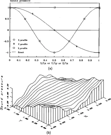
Some representative eigenmodes obtained from the

BEM-based eigenanalysis algorithm are shown in terms of profile curves and 3-D hidden line graphs from Figs. 6-9. Every eigenvector has been normalized with respect to the largest amplitude. Evidently, the calculated eigenmodes ap- pear to agree very well with the exact solutions. In fact, the same BEM technique was also applied to a rigid spherical enclosure. Very good agreement was achieved between the numerical results and the exact solutions. The BEM-based technique again provides much higher accuracy than the

FEM-based technique. Since this do•s not add up any new conclusion, the numerical results are omitted here.

In addition to the previously mentioned rectangular room, a car interior is selected as the second example for testing the usefulness of the BEM-based eigenanalysis tech- nique when applied to a more practical situation where an odd-shaped boundary is present. The motivation of explor- ing this problem stems from the need of optimizing acoustic performance that could be important for noise control in automobile design.

Consider a car-shaped enclosure with the dimensions as shown in Fig. 10. Since no analytic solution is available for this car interior of complex geometry, comparison of eigen- values and eigenmodes can only be made between numerical

Sing•lar values 1.6 1.4 I o 0.8 0.6

0.

,t

'•"-•.._..._•,_.•_....,...••_,

0

FIG. 4. Singular values associated with the repeated eigenvalue 3.14 corre-

sponding to the modes (0, 0, 1 ), (0, 2, 0), and (3, 0, 0).

Singular values O. 0. 0. 0. 0 0 10 20 30 40 50 60 70 Number

FIG. 5. Singular values associated with the eigenvalue 1.05 corresponding to the single mode ( 1, 0, 0).

-0 5 X_prof•le Y_profile Z_profile Exact I _{I I I I ! I I} 0 01 02 0.3 0.4 0.5 0.6 07 0.8 0.9 X/Lx ,)r Y/l,y or Z/Lz (a) (•)

FIG. 6. Eigenmode ( 1, 0, 0) associated with the eigenvalue 1.05 in the case

of a rectangular room. •o!ind presstire I -0.5

ß i t i I z

FIG. 8. Eigenmode (2, 1, 0) associated with the eigenvalue 2.62 in the case of a rectangular room. pressure 05 -0.5 X_profile Y_profile Z_proflle Exact i i i I i i i i i O. l 02 0.3 0.4 0 5 0 B 0.7 0.8 0.9 X/Lx or Y/Ly or Z/Lz (•) (b)

FIG. 7. Eigenmode ( 1, 1, 0) associated with the eigenvalue 1.89 in the case

of a rectangular room.

•OHIi(l i)re•511 l'e

0 O. 1 0 2 0.3 0.4 0 5 0 6 () 7 0 8 0.9 1

X/Lx or Y/l,y or Z/Lz

(•)

FIG. 9. Eigenmode (3, 0, 0) associated with the eigenvalue 3.14 in the case

FIG. 10. The mesh and the dimensions of a car interior in the numerical

simulation.

methods. In this simulation, the mesh of BEM consists 90 rectangular boundary elements with 272 colocation points

and the mesh of the FEM consists of 54 brick elements with

376 colocation

points.

The problem

size

is appreciably

larger

It should be noted that the solid angles at corners and

edges of the car interior do not have theoretical values. The numerical technique presented in Sec. I must be utilized to

solve for the solid angle parameter ai associated with each

node.

From the simulation results, the BEM-based eigenana- lysis technique does exhibit its effectiveness in extracting eigenmodes for an enclosure of complex geometry. In Table II, the eigenvalues of the first five modes obtained from the BEM-based eigenanalysis technique are compared with those obtained from the FEM. Excellent agreement of eigen- values has been achieved between the BEM and the FEM

(the errors are all within 2%). The corresponding eigen-

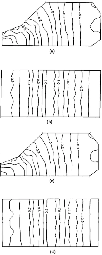
modes are shown in terms of contour graphs from both the side views and the top views (see Figs. 11-15). Differences between the mode shapes obtained from these two numerical methods are barely noticeable. Except for some figures, e.g., Figs. 1 ! (b) and 12(b), which show wavy contours instead of perfect straight lines (due to discretization errors), the mode shapes appear to be satisfactorily computed. No con- tours appear in Fig. 13 (a) and (c) because, for this mode,

(b)

(d)

TABLE II. Comparison of eigenvalues of the sound field in the car interior.

Eigenvalue k e

Mode BEM FEM

FIG. 11. The first eigenmode of the sound field in the car interior. (a) Pres- sure contours in plane y = 0, obtained from the BEM. (b) Pressure con- tours in plane z = 0, obtained from the BEM. (c) Pressure contours in plane y = 0, obtained from the FEM. (d) Pressure contours in plane z = 0,

obtained from the i•EM.

1 0.70 0.71

2 1.20 1.22

3 1.40 1.38

4 ' 1.48 1.49

5 1.57 1.55

the pressures of all nodes on this plane are supposed to be of a constant level.

Some comments can be made from the computed results in regard to the nature of the mode shapes. Similarities are

(b) (c) (b) (c)

,

FIG. 12. The second eigenmode of the sound field in the car interior. (a) Pressure contours in plane y = 0, obtained from the BEM. (b) Pressure contours in plane z = 0, obtained from the BEM. (c) Pressure contours in plane y = 0, obtained from the FEM. (d) Pressure contours in plane z = 0,

obtained from the FEM.

0.4. • - 0.4 •

0,2 '--T

(d)

FIG. 13. The third eigenmode of the sound field in the car interior. (a) Pressure contours in plane y = 0, obtained from the BEM. (b) Pressure

contours in plane z = 0, obtained from the BEM. (c) Pressure contours in plane y = 0, obtained from the FEM. (d) Pressure contours in plane z = 0,

obtained from the FEM.

found between, for example, Figs. !1 (b) and 12(b) as well as Figs. 11 (a) and 15 (a). This implies these two modes are

of identical order in one coordinate surface, but of different

order in the others (although these coordinate surfaces al-

ways

exist,

they

do not have

analytical

forms

due

to the com-

plex

geometry).

The higher

the resonance

frequency

is, the

more variations there are in the mode shapes, e.g., the sym-

metric

mode

in Fig. 11

(b) versus

the antisymmetric

mode

in

(b)

(c)

(b)

(d)

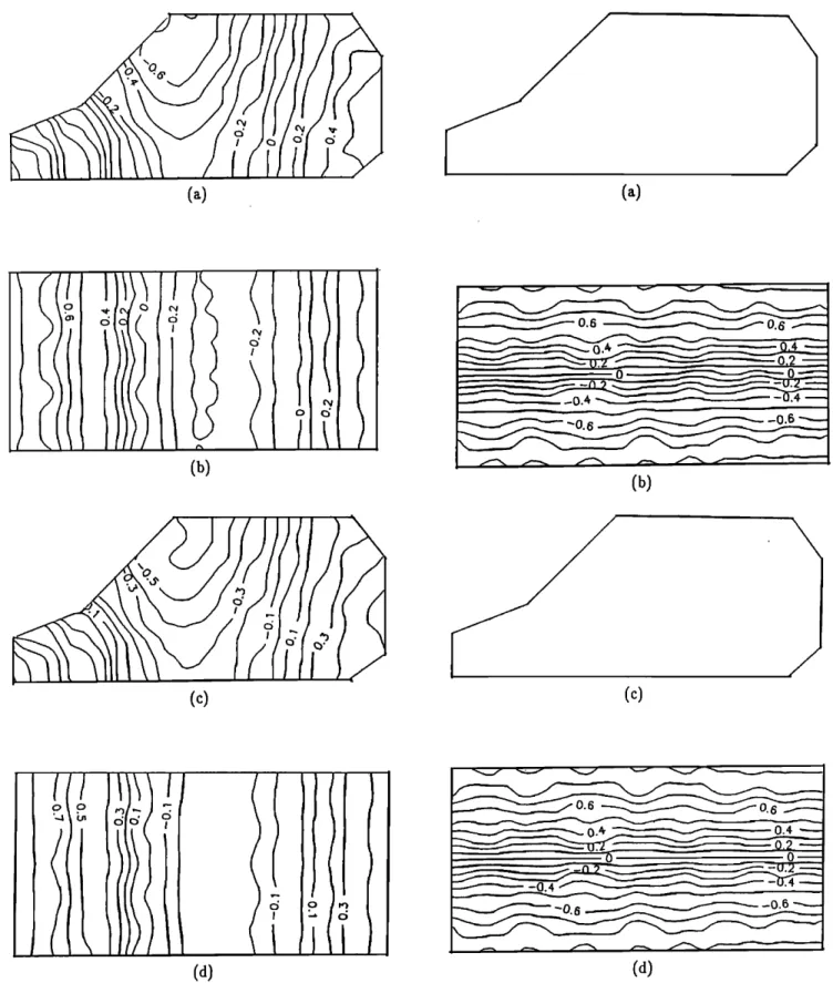
FIG. 14. The fourth eigenmode of the sound field in the car interior. (a) Pressure contours in plane y = 0, obtained from the BEM. (b) Pressure contours in plane z = 0, obtained from the BEM. (c) Pressure contours in plane y = 0, obtained from the FEM. (d) Pressure contours in plane z -- 0,

obtained from the FEM.

Fig. 15 (b). On the other hand, orthogonality is readily ob- served from some contour figures, e.g., Figs. 11 (b) and 13 (b). This is a natural consequence of the self-adjoint and undamped eigenvalue problem considered herein.

(d)

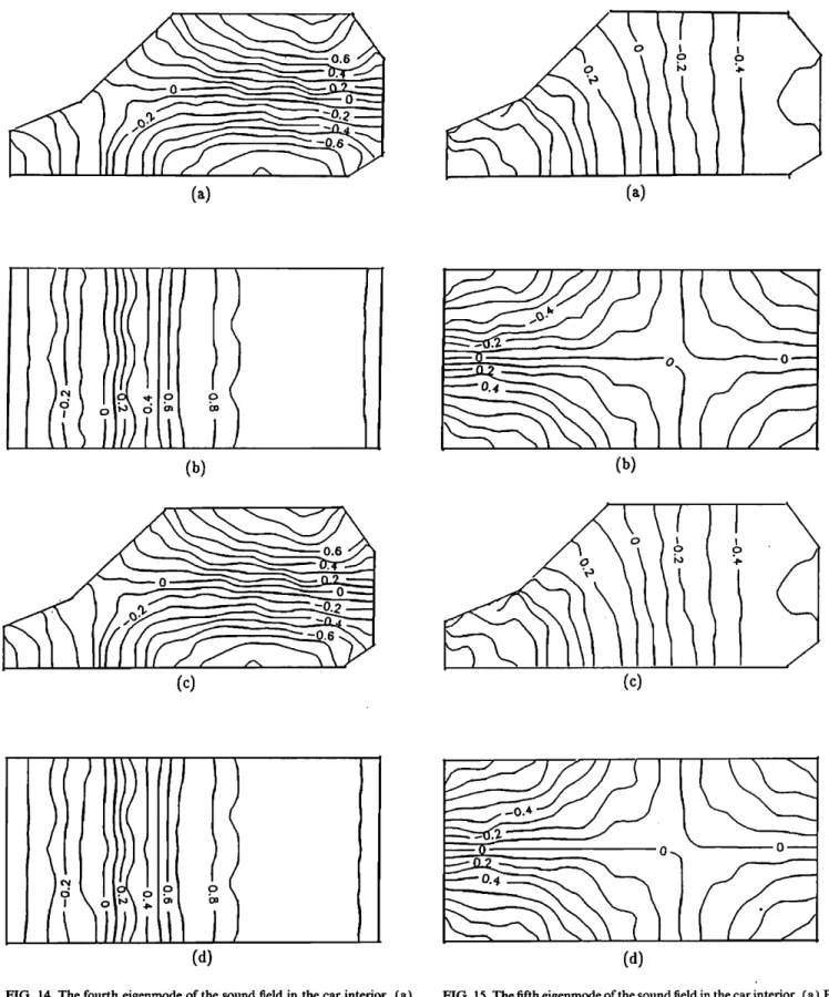
FIG. 15. The fifth eigenmode of the sound field in the car interior. (a) Pres-

sure contours in plane y = 0, obtained from the BEM. (b) Pressure con- tours in plane z- 0, obtained from the BEM. (c) Pressure contours in plane y = 0, obtained from the FEM. (d) Pressure contours in plane z -- 0,

obtained from the FEM.

Questions may be raised regarding the use of the eigen- modes associated with a car interior. To the author's knowl- edge, one possible application is optimizing the acoustical performance for the purpose of noise control. For example,

judging from the pressure distribution in Fig. 15 (a), one may want to apply certain sound absorption measures to the regions around the front end as well as the rear part of the car interior where pressure magnitudes reach maxima if the fre- quency of the major concern is around 38 Hz. In addition, if

a hi-fi stereo system is to be installed in the car, one may

prefer a relatively uniform distribution, e.g., the pressure field in Fig. 13, of the sound field over a nonuniform one.

Under these circumstances, the BEM-based eigenanalysis

technique serves as a useful simulation tool for extracting

resonance frequencies and mode shapes of sound fields be- fore an actual prototype of a car is built.

III. CONCLUSIONS

A BEM-based eigenanalysis technique is presented in this study for extracting eigenmodes of sound fields in arbi- trarily shaped enclosures. Complete procedures involved in numerical implementation are demonstrated in details. The method of singular value search is utilized to determine nat- ural frequencies and mode shapes of sound pressure distribu- tion (associated with not only distinct but also repeated eigenvalues).

The BEM eigenanalysis technique has been verified through comparisons between the numerical results and the

exact solution if available. In addition, the BEM results are

also compared with those obtained from the FEM in order to explore the numerical performance. The BEM approach, in- terestingly enough, achieves much higher accuracy than the FEM despite the fact that the errors of the higher modes are always greater than those of the lower ones, regardless of which numerical method is used. It is of no doubt that these numerical schemes will lose their effectiveness at high-fre- quency ranges due to increasing density of eigenmodes.

The sizes of the resulting system matrices of the BEM are always smaller than those of the FEM because the re- quired meshes for the BEM are simpler than those for the FEM. This should become more pronounced for the enclo- sures of large volume-to-surface ratio in a three-dimensional space. This reduction of problem size facilitates generation of boundary meshes with reference to the design changes regarding boundary conditions and geometry of an enclo- sure. This attractive feature makes BEM-based eigenanaly- sis technique a useful simulation tool before an actual proto- type is built. Note that the BEM, while dimensionally

smaller than the FEM, takes more CPU time than the FEM

because of full and asymmetric nature of assembled matri- ces. More research is required for improving the efficiency of the BEM-based approach.

Although the boundaries of enclosures have been as-

sumed perfectly rigid in this study, the BEM-based eigenan- alysis technique can be easily extended to the other types of

boundary such as the pressure-release type, the impedance

type, and the mixed type. These aspects will be explored by

more numerical as well as experimental investigations in the future research.

ACKNOWLEDGMENTS

The author is indebted to the graduate student Yuan- long Lan for the computer implementation of the concepts

developed in this research. The work was supported by the

National Science Council in Taiwan, Republic of China un- der the project number NSC80-040 l-E009-13.

A.D. Pierce, Acoustics (McGraw-Hill, New York, 1981 ).

L. E, Kinsler, A. R. Frey, A. B. Coppens, and J. V. Sanders, Fundamen-

tals of Acoustics (Wiley, New York, 1982).

R. Hickling, D. A. Feldmaier, F. H. K. Chen, and J. S. Morel, "Cavity

Resonances in Engine Combustion Chambers and Some Applications," J.

Acoust. Soc. Am 73, 1170-1178 (1983).

p.M. Morse and K. U. Ingard, Theoretical Acoustics (McGraw-Hill, New York, 1968).

G. F. Roach, Green's Functions (Cambridge U.P., New York, 1982). R. E. Kleinman and G. F. Roach, "Boundary Integral Equations for The

Three-Dimensional Helmholtz Equation," SIAM Rev. 16, 216-236

(1974).

p. K. Banerjee and R. Butterfield, Boundary Element Methods in Engi-

neering Science (McGraw-Hill, New York, 1981 ).

G. DeMey, "Calculation of the Eigenvalues of Helmholtz Equation by An

Integral Equation," Int. J. Num. Meth. Eng. 10, 56-66 (1976).

M. Kitahara, Boundary Integral Equation Methods in Eigenvalue Prob-

lems of Elastodynamics and Thin Plates' (Elsevier, Amsterdam, 1985).

2o E. Dokumaci, "A Study of The Failure of Numerical Solutions in Bound-

ary Element Analysis of Acoustic Radiation Problems," J. Sound Vib.

139, 83-97 (1990)

B. Noble and J. W. Daniel, Applied Linear Algebra (Prentice-Hall, Engle- wood Cliffs, NJ, 1988).

22 j. $. Arora, Introduction to Optimum Design (McGraw-Hill, New York, 1989).

•3 A. Craggs, "The Use of Simple Three-Dimensional Acoustic Finite Ele-

ments for Determining the Natural Modes and Frequencies of Complex Shaped Enclosures," J. Sound Vib. 23, 331-339 (1972).

24 M. Petyt, J. Lea, and G. H. Koopmann, "A Finite Element Method for

Determining the Acoustic Modes of Irregular Shaped Cavities," J. Sound

Vib. 45, 495-502 (1976).

R. K. Sigman and B. T. Zinn, "A Finite Element Approach for Predicting Nozzle Admittances," J. Sound Vib. 88, 117-131 (1983).