基於色彩及深度影像之即時人形偵測系統設計

國 立 交 通 大 學

電控工程研究所

碩 士 論 文

基於色彩及深度影像之

即時人形偵測系統設計

Real-time Human Detection System Design

Based on RGB-D Images

研 究 生：林谷穎

指導教授：陳永平 教授

基於色彩及深度影像之

即時人形偵測系統設計

Real-time Human Detection System Design

Based on RGB-D Images

研 究 生：林谷穎 Student：Ku-Ying Lin

指導教授： 陳永平 Advisor：Professor Yon-Ping Chen

國 立 交 通 大 學

電控工程研究所

碩 士 論 文

A Thesis

Submitted to Institute of Electrical Control Engineering College of Electrical and Computer Engineering

National Chiao Tung University In Partial Fulfillment of the Requirements

For the Degree of Master In

Electrical Control Engineering June 2013

Hsinchu, Taiwan, Republic of China

基於色彩及深度影像之

即時人形偵測系統設計

學生: 林谷穎 指導教授: 陳永平 教授

國立交通大學電控工程研究所

摘 要

本篇論文針對人形偵測提出一個即時人形偵測系統，此系統基於 Kinect 所 產生的彩色及深度串列影像來找出影像中的人形。此系統分成四個部分，包括感 興趣區域的選擇、特徵擷取、人形識別以及靜態人形之檢查。首先，根據人在行 走或站立時之人形特性，進而利用直方圖投影、連通物件標示法以及移動物體區 分法來選擇出感興趣的區域。然後，藉由雙線性插值法將感興趣的區域標準化， 以及透過方向梯度直方圖來擷取人形的特徵。再來是採用支持向量機或類神經網 路來訓練出 Leeds Sports Pose 資料集的分類器，並利用此分類器來辨識人形。最 後，檢查在影像中是否有包含任何靜態的人形而後辨識它。從實驗結果可知，本 論文所設計之人形偵測系統擁有即時且高準確率的特性。

Real-time Human Detection System Design

Based on RGB-D Images

Student：Ku-Ying Lin Advisor：Prof. Yon-Ping Chen

Institute of Electrical Control Engineering

National Chiao-Tung University

ABSTRACT

This thesis proposes a real-time human detection system based on RGB-D images generated by Kinect to find out humans from a sequence of images. The system is separated into four parts, including region-of-interest (ROI) selection, feature extraction, human shape recognition and motionless human checking. First, the histogram projection, connected component labeling and moving objects segmentation are applied to select the ROIs according to the property that human is walking or standing with motion. Second, resize the ROIs based on the bilinear interpolation approach and extract the human shape feature by Histogram of Oriented Gradients (HOG). Then, support vector machine or artificial neural network is adopted to train the classifier based on Leeds Sports Pose dataset, and human shape recognition is implemented by the classifier. Finally, check whether the image contains any motionless human, and then recognize it. From the experimental results, the system could detect humans in real-time with high accuracy rate.

Acknowledgement

在研究所的兩年中，首先我要感謝我的指導教授-陳永平教授，在陳 永平老師的諄諄教誨下，讓我在口語表達能力、思考邏輯以及英文聽說讀 寫上都有大幅的進步，另外在求學路上以及人生方向提供了我許多寶貴建 議，最終也使我得以順利完成此篇論文，實則受益良多。還要感謝世宏、 振方、榮哲、孫齊、崇賢以及咨瑋學長在我遇到問題時能夠幫助我、引導 我解決問題。最後，謝謝口試委員-林昇甫教授與張浚林教授提供寶貴的 意見，讓整篇論文更加仔細而完整。 另外，感謝可變結構控制實驗室的兆村、仕政、宣竣、仁傑、惠琪、 御旻以及冠銘同學的陪伴與學習，讓我充實了研究所兩年的歲月。最後， 感謝我的父母、家人和所有我的朋友，給予我支持與鼓勵。謝謝你們！ 謹以此篇論文獻給所有照顧我、關心我的人。 林谷穎 2013.6

Contents

Chinese Abstract ... i English Abstract ... ii Acknowledgement ... iii Contents ... iv List of Figures ... vi

List of Tables ... viii

Chapter 1 Introduction ... 1

1.1 Preliminary ... 1

1.2 System Overview... 2

1.2.1 Hardware Architecture ... 2

1.2.2 Software Architecture ... 4

Chapter 2 Related Works ... 6

2.1 Human Detection Methods ... 6

2.1.1 Foreground Segmentation ... 6

2.1.2 Feature Extraction ... 7

2.1.3 Human Recognition ... 8

2.2.1 Introduction to ANNs ... 10

2.2.2 Back-Propagation Network ... 12

2.3 Support Vector Machine ... 16

2.4 Morphology Operations ... 19

2.4.1 Dilation and Erosion ... 19

2.4.2 Opening and Closing ... 22

Chapter 3 Intelligent Human Detection ... 24

3.1 ROI Selection ... 25

3.1.1 Histogram Projection ... 25

3.1.2 Connected Component Labeling ... 27

3.1.3 Moving Objects Segmentation ... 30

3.2 Feature Extraction ... 31

3.2.1 Normalization ... 32

3.2.2 Histogram of Oriented Gradient ... 34

3.3 Human Shape Recognition ... 36

3.4 Motionless Human Checking ... 42

Chapter 4 Experimental Results ... 44

4.1 ROI Selection ... 44

4.2 Feature Extraction ... 49

4.4 Motionless Human Checking ... 53

Chapter 5 Conclusions and Future Works... 55

Reference ... 57

List of Figures

Fig-1.1 (a) Example of the depth image (b) Example of the color image ... 3

Fig-1.2 Software architecture ... 4

Fig-2.1 Examples of Haar-like features ... 7

Fig-2.2 Basic structure of ANNs ... 11

Fig-2.3 Multilayer feed-forward network ... 12

Fig-2.4 Neural network with one hidden layer ... 13

Fig-2.5 A set of 2D-points which belong to one of two classes ... 16

Fig-2.6 Multiple straight lines separate the set ... 17

Fig-2.7 The optimal separating hyperplane with maximum margin ... 17

Fig-2.8 Example of dilation operation ... 20

Fig-2.9 Example of erosion operation ... 21

Fig-2.11 Example of closing operation ... 23

Fig-3.1 Flowchart of the human detection system ... 24

Fig-3.2 Example of the depth image and color image generated by Kinect ... 25

Fig-3.3 Scanning the image ... 28

Fig-3.4 Example of 4-pixel CCL (a) Binary image (b) Labeling (c) Componentizing ... 29

Fig-3.5 (a)Previous frame (b)Current frame (c) The difference of frames ... 31

Fig-3.6 (a)The result of nearest neighbor interpolation approach (b)The result of bilinear interpolation approach ... 33

Fig-3.7 The parameters of HOG for computation... 34

Fig-3.8 (a) the horizontal operation (b) the vertical operation ... 35

Fig-3.9 The example of HOG ... 36

Fig-3.10 Some examples of original dataset ... 37

Fig-3.11 Some examples of normalized dataset ... 37

Fig-3.12 The distribution of training data of SVM ... 38

Fig-3.13 The classifier for human shape recognition of SVM ... 39

Fig-3.14 The structure of neural networks ... 40

Fig-3.16 The process of parameters of ROI storing... 42

Fig-4.1 The process and result of ROI selection ... 45

Fig-4.2 Comparing difference of depth and gray images ... 47

Fig-4.3 ROI selection only by moving objects segmentation and CCL ... 49

Fig-4.4 Some original data and normalized original data ... 49

Fig-4.5 Some normalized test data of subjects for experiment ... 50

Fig-4.6 Three continue frames of motionless human checking ... 54

Index of Tables

Table 1.1 Specification for the Kinect ... 3

Table 4.1 TP, FP, FN, TN table ... 52

Table 4.2 The performance and average executing time of two approaches ... 53

Chapter 1

Introduction

1.1 Preliminary

In recent years, the techniques for human detection in images or videos have been studied widely and intensively in a variety of applications such as intelligent vehicles, video surveillance and advanced robotics. In the field of advanced robotics, it is devoted to develop a robot which could take care of children and interact with them. In order to provide the information of interaction between robots and children, it is required to determine whether children are in the image or whether the objects in front of the robot are children. Thus, human detection plays an important and essential role for the development of robots.

Nonetheless, detecting humans in an image is often a challenging task. First, human may appear in various shapes, poses, clothes, etc. Hence, it is difficult to handle all the situations through any simple models. Second, when more than one human are in the image, humans may occlude each other or with other objects, like desks, chairs and shelves, and reveal only parts of their bodies. Therefore, it is required to detect human correctly even though the body is partially occluded. Third, the detection process should be influenced by the distances between objects and camera. With a longer distance, an object has a smaller size in the image which makes the detection process more difficult. Finally, if the camera is static, it is easy to establish a background model to implement foreground segmentation. However, when the camera is installed on a moving platform, it is hard to segment foreground using conventional techniques.

According to the above reasons, a lot of problems exist in human detection and recently several detection methods have been proposed to solve these problems. In general, the overall process is usually separated into three main steps, including foreground segmentation, feature extraction and human recognition. First, foreground segmentation is implemented to filter out non-human background regions. Hence, only foreground regions are processed to speed up the detection process. Then, feature extraction is implemented to efficiently and correctly extract appropriate human features, like edges, skeletons, etc. Finally, based on the extracted features, human recognition is applied to recognize the human shape and complete the human detection process. The related techniques and methods would be introduced in the following chapters.

1.2 System Overview

This section would briefly introduce the hardware architecture and software architecture of the system for the human detection algorithm.

1.2.1 Hardware Architecture

The hardware of the system is based on the Personal Computer (PC) and Xbox Kinect to obtain image frames, including color image and depth image. The

specification of Kinect is shown in Table 1.1 and the specification of the PC is Intel® Core™ i3-2100, 4GB random-access memory, and Windows 7 64-bit operation system. Fig-1.1 gives an example of depth image and color image. In the depth image, the lower pixel value of an object implies the shorter distance between the object and Kinect. Moreover, for the areas where the depth sensor cannot measure the depth,

their pixel values would be offset to zero and revealed as dark areas. In the color image, the pixel in RGB color space is represented by the format in 32 bits. After PC receives the frames from Kinect, the human detection and tracking will be further implemented by using C/C++.

Table 1.1 Specification for the Kinect [1, 2]

Item Array specification

Color and depth Effective range is 1.2m ~ 3.6m

Viewing angle 43 degrees vertical by 57 degrees horizontal field of view

Frame rate 30 frames per second (FPS)

Resolution of depth QVGA (320×240)

Resolution of color VGA (640×480)

(a) (b) Fig-1.1 (a) Example of the depth image (b) Example of the color image The experimental environment is our laboratory and building. Moreover, the Kinect camera is set at about 100cm height. However, there are two limitations when implementing the human detection system: First, the detection distance is between

1.2m to 3.6m due to the hardware limitation of Kinect. Second, the Kinect camera always adjusts white balance automatically.

1.2.2 Software Architecture

For the software architecture, the image shown in Fig-1.2 is the flowchart of the proposed system. For a start, the system obtains the depth images and color images from Kinect, and then it selects the region-of-interest (ROI) through the color and depth (RGB-D) information. ROI selection could be divided into three sub-steps: histogram projection, connected component labeling (CCL) and moving objects segmentation. After ROI selection, the size of the ROI would be normalized based on the bilinear interpolation no matter how large it is. Afterword histogram of oriented gradients (HOG) is implemented to be human feature descriptors. At the next step, the overall features are passed to the human shape recognition system to judge whether the ROIs contain human or not. Finally, the system check if any motionless human exists in the current frame, and regard it as new ROI in next frame.

The remainder of this thesis is organized as follows: Chapter 2 describes the related works of the algorithm in the system. Chapter 3 introduces the above-mentioned human detection system in detail. Chapter 4 shows the experimental results. Chapter 5 is the conclusions of the thesis and the future works.

Chapter 2

Related Works

2.1 Human Detection Methods

In recent years, many human detection approaches have been developed. In general, there are three parts of human detection system, foreground segmentation, feature extraction and human recognition.

2.1.1 Foreground Segmentation

In order to simplify image scanning, the foreground segmentation is used to filter out the background of an image and separate the interested regions, regions of interest (ROI), from the original image. There are several methods to segment foreground such as optical flow method [3-5], background subtraction [6-9]. For the optical flow method, the relative motion of a camera to the scene results in optical flow, treated as the pattern of apparent motion of objects, surfaces, and edges in a visual scene. This method can detect interesting foreground regions accurately, but it costs lots of time on computation and is difficult to realize in real-time. As for the background subtraction, it has been widely used in computer vision systems to detect moving objects in videos. In this method, the difference between a current frame and a reference frame is calculated, and then the objects of interest are retrieved according to a threshold. But the background model must be updated continuously due to the illumination change or changeable background.

Furthermore, some methods are used with the special techniques such as infrared cameras [10] or depth sensors [10-15]. Based on the depth information, it is

feasible to generate a faithful background model for the scene, which can be used to detect foreground objects, because it is not sensitive to illumination change and distance influence. Therefore, this thesis uses depth information to implement foreground segmentation of the humans in the realistic environment.

2.1.2 Feature Extraction

As soon as the foreground regions are segmented, different combinations of features and classifiers will be applied to distinguish human shape from other objects. The purpose of feature extraction is to extract human-related features to increase detection rate. Besides, there are many kinds of features which could be used to recognize the human shape. For example, one of the features is on the basis of image gradient, like the histogram of oriented gradient (HOG) [16, 17], edge information [10, 12, 13], and Haar-like features [18]. Fig-2.1 shows some of Haar-like features. Since the image gradient reflects the direction change in the intensity or color in a digital image, the boundary of objects including the human shape information could be found and extracted from image gradient. The other feature is based on the motion [13, 18], because humans often perform periodic motion, like walking. Therefore, humans could be separated from other objects by their motion periodicity. As to the other features, such as texture [12], skeleton [19], scale-invariant feature [20], and so on, they are often applied in human detection. In practice, it is common to use more than one feature to implement human detection due to the high variation of human appearance.

2.1.3 Human Recognition

After feature extraction, the system can separate the human from other objects through many kinds of features. In this way, the system can recognize the humans by the techniques of machine learning such as support vector machine (SVM) [7, 16], Adaptive Boosting (AdaBoost) [18, 21], artificial neural network (ANN) [10, 22, 23], and so on. The main advantages of machine learning are the learning ability and the tolerance of variation. Nevertheless, the system often requires a large amount of training samples in order to learn how to judge human and non-human in machine learning. With regard to support vector machines, they can determine the best discriminant support vectors according to the minimum empirical classification error and the maximum geometric margin. As for the Adaptive Boosting, it constructs a classifier based on a weighted linear combination of selected features for the lowest error on the training set consisting of human and non-human. For the artificial neural networks, they have been successfully applied to pattern recognition and data processing. For example, the artificial neural networks are able to model complex relationship between inputs and outputs or find patterns for judging human and non-human.

Besides, the technique of template matching [11, 14, 24-27] is also popular in human detection. When compared with machine learning, the template matching is easier to implement and costs lower computation time, but suffers from less variation tolerance. For example, the system in [28] uses a set of templates to form a hierarchical structure [27, 29] according to the similarity between each pair of models. The root of the structure, like a tree, is situated by the model with the highest similarity while the more particular models will be leaves of the tree. As a result, it

would improve the variation tolerance without increasing the computation time because of its hierarchical structure. Nonetheless, it is difficult and inefficiency to collect the templates and determine the similarity between each pair of models.

Except the above methods which directly detect the whole human shape, another methods use part of the templates [21, 24, 26, 27, 30] to match human shape in order to get higher detection rate and handle the occlusion problems. These methods decompose the structure of a human body into a number of body parts, where each part is described by a small set of part templates and would contribute differently to recognition of the whole human body. Therefore, the methods could detect different body parts rather than detect the whole human shape. In the part templates matching, it could reduce the variation of human appearance by a street and resolve partial occlusion problem; however, it would result in more computational cost and decrease the detection speed.

2.2 Neural Network

Artificial neural networks (ANNs) are systems that are constructed to make use of some organization of principles resembling those of the human brain. They represent the promising new generation of information processing system. ANNs are good at tasks such as pattern matching, classification, function approximation and optimization, while traditional computers are inefficient at these tasks, especially pattern-matching. However, traditional computers are faster in algorithmic computation and precise arithmetic operations.

2.2.1 Introduction to ANNs

The human nervous system consists of a large amount of neurons. Each neuron includes four parts: somas, axons, dendrites and synapses, and is capable of receiving, processing, and passing signals from one to another. To mimic the characteristics of the human nervous system, recently investigators have developed an intelligent algorithm, called artificial neural networks (ANNs). Through proper learning processes, ANNs have been successfully applied to some complicated problems, such as image analysis, speech recognition, adaptive control, etc. In this thesis, the ANNs will be adopted to implement human detection via intelligent learning algorithms.

The basic structure of a neuron is shown in Fig-2.2, whose input-output relationship is described as 1 n i i i y f w x b =   = _ + _ 

∑

 (2.1)

where f( )⋅ is the activation function, w_i is the weight of the input x_i and b is the bias. There are three common activation functions, including linear function, log-sigmoid function and tan-sigmoid function, which are described as below:

i. Linear function

( )

f x =x _(2.2)

ii. Log-sigmoid function

1 ( ) 1 x f x e− = + _(2.3)

iii. Tan-sigmoid function

( ) x x x x e e f x e e − − − = + (2.4)

weighted inputs and the bias are propagated to the activation function to determine the activation level of the neuron.

Generally, a multilayer feed-forward network is usually divided into three kinds of layers, including one input layer, one output layer, and at least one hidden layer. Take Fig-2.3 as an example, it shows a neural network with one input layer, one output layer and two hidden layers. Each layer is based on neurons whose basic structure is depicted in Fig-2.2. The input layer receives signals from the outside world, and then delivers their responses layer by layer. From the output layer, the overall response of the network can be obtained. As expected, a neural network with multi-hidden layers is indeed able to deal with more complicated problems compared to that with a single hidden layer. Nonetheless, the training process of multi-hidden layer networks may be more tedious.

Fig-2.3 Multilayer feed-forward network

In addition to the structure, it is still demanded to determine the way of training for a neural network. In general, the training could be separated into two kinds of learning process, supervised and unsupervised [31]. The main difference between them is whether the set of target outputs is given or not. Training via supervised learning is mapping a given set of inputs to a specified set of target outputs and adjusts weights according to a pre-assigned learning algorithm. On the other hand, unsupervised learning could self-organize a neural network without any target outputs, and modify the weights so that the most similar inputs can be assigned to the same group. In this thesis, the neural network is designed for image recognition based on supervised learning; as a result, both the input and target images are necessary.

2.2.2 Back-Propagation Network

familiar method to train artificial neural networks for executing a given task. The BP algorithm proposed in 1986 by Rumelhart, Hinton and Williams, is based on the gradient steepest descent method for updating the weights to minimize the total square error of the output. In order to explain the BP algorithm clearly, take a neural network

with one hidden layer as an example shown in Fig-2.4. Let the inputs be x_i,

1, 2, ,

i=  I, and the outputs be y_o, o=1, 2,,O, where I and O are the total numbers of input and output neurons, respectively. In the hidden layer, it owns J hidden neurons for receiving information from input layer and sending out the response to the output layer. Moreover, three kind of layers are connected by two sets of weights v and _ij w , where _jo v connects the i-th input node to the k-th hidden _ij

node, and w connects the k-th hidden node to the j-th output node. _jo

Considering the neural network example in Fig-2.4 again, the BP algorithm for supervised learning is generally processed step by step as below:

A. Set the initial weight and bias value of the network at random.

B. Set the maximum tolerable error E_max and the learning rate η between 0.1 and 1.0 to reduce the computing time or increase the precision.

C. Input the training data of input x=[x₁ x₂  x_i  x_I]T and the target data of desired outputt=[t₁ t₂  t_o  t_O]T.

D. Calculate each output of the J neurons in hidden layer

1 , 1, 2, I j h ij i i h f v x j J =   = _{ } = 

∑

  (2.5)

where fh( )⋅ is the activation function of the hidden layer, and each output of

the O neurons in output layer

1 , 1, 2, J o y jo j j y f w h o O =   = _{ } = 

∑

  (2.6)

where f_y( )⋅ is the activation function of the output layer.

E. Calculate the error function between network output and desired output by

following equation 2 2 1 1 1 1 1 ( ) ( ) [ ( )] 2 2 O O J o o o y jo j o o j E w d y d f w h = = = =

∑

− =

∑

−

∑

(2.7)

where d_o is the desired output.

F. According to gradient descent method, determine the correction of weights as

o jo jo j jo o jo y E E w h w y w

η

∂

η

∂ ∂

ηδ

∆ = − = − = ∂ ∂ ∂ (2.8) and 1 O j o ij ijo i o ij o j ij h y E E v x v y h v η η ηδ = ∂ ∂ ∂ ∂ ∆ = − = − = ∂

∑

∂ ∂ ∂ (2.9) where 1 ( ) J jo o o y jo j j d y f w h δ =  _′  = −       

∑

 (2.10) and 1 1 1 ( ) O J I ijo o o y jo j jo h ij i o j i d y f w h w f v x δ = = =  _′   _′  = _ − _{    }        

∑

∑

∑

(2.11)

G. Propagate the correction backward to update the weights as below

( 1) ( ) ( 1) ( ) w n w n w v n v n v + = + ∆   _{+ = + ∆}  (2.12)

H. Check whether the overall training data set have learned already or not.

Networks learn the overall training data set once considered a learning circle. If the networks don’t go through a learning circle, return to Step-C; otherwise, go to the next step, Step-I.

I. Check whether the network converges or not. If

max

E <E , terminate the training

process; otherwise, begin another learning circle by going to Step-A.

BP learning algorithm can be used to model various complicated nonlinear functions. In recent years, the BP learning algorithm is successfully applied to many domain applications, such as pattern recognition, adaptive control, clustering problem, etc. In the thesis, the BP algorithm was used to learn the input-output relationship for clustering problem.

2.3 Support Vector Machine

In machine learning, support vector machines (SVM) are supervised learning models with associated learning algorithms that analyze data and recognize patterns, used for classification and regression analysis. The basic SVM takes a set of input data and predicts that each given input is under which one possible class of the output, making it a non-probabilistic binary linear classifier. Given a set of training examples, each marked as belonging to one of two categories, an SVM training algorithm builds a model that assigns new examples into one category or the other. In addition to performing linear classification, SVM can efficiently perform non-linear classification using what is called the kernel trick, implicitly mapping their inputs into high-dimensional feature spaces.

Taking a graphic example for more detailed illustration, Fig-2.5 is a linearly separable set of 2D-points which belong to one of two classes, and then find a separating straight line.

Fig-2.5 a set of 2D-points which belong to one of two classes

By the above-mentioned, there are multiple separating straight lines passing muster to offer a solution to the problem in Fig-2.6. However, a line is bad if it passes

too close to the points because it will be noise sensitive and it will not generalize correctly. Therefore, SVM algorithm should be to find the line passing as far as possible from all points.

Fig-2.6 multiple straight lines separate the set

In Fig-2.7, the operation of the SVM algorithm is based on finding the hyperplane that gives the largest minimum distance (maximum margin) to the training examples. Therefore, the optimal separating hyperplane maximizes the margin of the training data.

As for a hyperplane, the notation is formally defined as

T 0

f(x) =β + β x (2.13)

where β is known as the weight vector and β₀ as the bias. The optimal hyperplane can be represented in an infinite number of different ways by scaling of β and β₀. As a matter of convention, among all the possible representation of the hyperplane, the one chosen is

1 = T 0

β + β x (2.14)

where x symbolizes the training examples closest to the hyperplane. In general, the training examples that are closest to the hyperplane are called support vectors. This representation is known as the canonical hyperplane. Based on the concept of geometry, the distance between a point and a hyperplane ( ,β β₀) can be defined as

distance =

T 0

β + β x

β (2.15)

According to (2.14), for the canonical hyperplane, the numerator is equal to one and the distance to the support vectors is

support vectors 1 distance = = T 0 β + β x β β (2.16)

and recall that the margin introduced in Fig-2.7, here denoted as M, is twice the distance to the closest examples:

2

M

=

β

(2.17)

Finally, the problem of M maximizing is equivalent to the problem of minimizing a function L( )β subject to some constraints. The constraints model the requirement for the hyperplane to classify correctly all the training examples x_i, and can be formally described as

2 , 1 min , subject to ( ) 1, 2

L( )

=

y_{i i}

+

≥ ∀i 0 β β T 0

β

β

β x β

(2.18)

where y_i represents each of the labels of the training examples, and (2.18) is a problem of Lagrangian optimization [32]. Therefore, (2.18) can be solved using Lagrange multipliers [32] to obtain the weight vector and the bias of the optimal hyperplane. In this example, it only deals with lines and points in the Cartesian plane instead of hyperplanes and vectors in a high dimensional space. However, the same concepts apply to tasks where the examples to classify lie in a space whose dimension is higher than two.

2.4 Morphological Operations

The word morphology commonly denotes a branch of biology that deals with the form and structure of animals and plants. In image processing, mathematical morphology is a tool for extracting image components that are useful in the representation and description of region shape, such as boundaries, skeletons, and the convex hull.

2.4.1 Dilation and Erosion

This section will introduce two fundamental morphological operations, dilation and erosion [33], and many morphological algorithms are based on these two primitive operations. The dilation operation is often used to repair the gaps and defined as

ˆ

{ | ( )_z }

A⊕ =B z B ∩ ≠A φ (2.19)

translation of the set Bˆ by z. The result of dilation in (2.19) is the set of all displacement, z, such that Bˆ and A overlap at least one element. For example, Fig-2.8(a) shows a simple set A, and Fig-2.8(b) and Fig-2.8(c) are two structuring elements. Fig-2.8(d) is the dilation of A using the symmetric element B, and shown shaded. Similarly, Fig-2.8(e) is the dilation of A using the element C, and shown shaded. In Fig-2.8(d) and Fig-2.8(e), the dashed line shows the original set A and all points inside this boundary constitute the dilation of A. Therefore, we can find that the dilation region will extend more when the structuring element is larger.

Oppositely, to remove noise and irregular regions, the erosion operation is often used and defined as

{ | ( )z }

A BΘ = z B ⊆ A (2.20)

where A and B are sets in 2

Z , ( )B _z is the translation of set B by z. Unlike dilation,

which is an expanding operation, erosion shrinks objects in the image. Taking Fig-2.9 as an example, it shows a process similar to that shown in Fig-2.8. Fig-2.9 (a) shows a simple set A, and Fig-2.9(b) and Fig-2.9(c) are two structuring elements. Fig-2.9(d) and Fig-2.9(e) are the erosion of A using the elements B and C. Besides, from Fig-2.9(e) we can find that if an element is too large, the result of erosion will be almost empty.

2.4.2 Opening and Closing

As we have seen, dilation expands an image and erosion shrinks it. This section will introduce two other important morphological operations based on dilation and erosion, which are opening and closing [33]. Generally, opening can smooth the contour of an object, breaks narrow isthmuses, and eliminates thin protrusions. Closing, as opposed to opening, it fuses narrow breaks and long thin gulfs, eliminates small holes, and fills gaps in the contour, but it also tends to smooth sections of contours.

The opening operation is the dilation of the erosion of a set A by a structuring element B, defined as

( )

A BA = A BΘ ⊕B (2.21)

where Θ and ⊕ denote the erosion and the dilation operations, respectively. For example, Fig-2.10 is a simple geometric interpretation of opening operation. The region of A BA is established by the points of A that can be reached by any point of

B when B moves vertically or horizontally inside A. In fact, the opening operation can

be also expressed as

{( ) | ( )_{z z} }

A BA = B B ⊆ A (2.22)

where  �{ } denotes the union of all the sets inside the braces.

Similarly, the closing operation is simply the erosion of the dilation of a set A by a structuring element B, defined as

( )

A B• = A⊕ ΘB B (2.23)

where ⊕ and Θ respectively denote dilation and erosion operation. Fig-2.11 is also a geometric example which introduces closing operation. In the Fig-2.11, B is moved on the outside of the boundary of A. Besides, it will be shown that opening and closing are duals of each other, so having to move the structuring element on the outside is not unexpected.

Chapter 3

Human Detection Algorithm

Human detection system is implemented by four main steps as shown in Fig-3.1, including region-of-interest (ROI) selection, feature extraction, human shape recognition and motionless human checking. The system obtains the depth images and color images from Kinect, and then it selects the region-of-interest (ROI) through histogram projection, connected component labeling (CCL) and moving objects segmentation. After ROI selection, the size of the ROI would be normalized based on the bilinear interpolation no matter how large it is. Afterwards histogram of oriented gradients (HOG) is implemented to be human feature descriptors. At the next step, the overall features are passed to the human shape recognition system to judge whether the ROIs contain human or not. Finally, the system check if any motionless human exists in the current frame, and regard it as new ROI in next frame.

Fig-3.2(a) shows an example of the depth image generated by Kinect, which contains 320×240 pixels with intensity values normalized into 0-255. The intensity value indicates the distance between object and camera, and the lower intensity value implies the smaller distance. Besides, Fig-3.2(a) shows an example of the color image, which contains 320×240 pixels as well.

(a) (b)

Fig-3.2 Example of the depth image and color image generated by Kinect

3.1 ROI selection

In order to reduce computational cost, the foreground segmentation is required to filter out the background to gain the region of interest (ROI), that is, a human moving in the image. The system is designed to detect the moving objects from the temporal difference frame by frame, and based on the difference the system applies the histogram projection, connected component labeling (CCL) and the moving object segmentation to select the ROI and then increase the speed and detection rate.

3.1.1 Histogram Projection

implement histogram projection as the following steps. First, the system computes the histogram of all columns in depth image with intensity levels in the range [0, 255]. Let the histogram of i-th column in depth image be

0, 1, 2, 255,

[ ] , 1, 2,T , 320

i i i i i

h = c c c  c i=  (3.1)

where c_{k i,} is the number of pixels related to intensity k in the i-th column. Then, define the histogram image as

1 2 3 320 0,1 0,2 0,3 0,320 1,1 1,2 1,3 1,320 2,1 2,2 2,3 2,320 255,1 255,2 255,3 255,320 [ ] h h h h c c c c c c c c c c c c c c c c =         =                   H (3.2)

with size 320×256. Note that the histogram image H could be considered as the vertical distribution of objects or humans in the real world. However, there are a large amount of pixels of intensity k=0 due to the camera limitation, not able to detect the depth of objects near to the camera or the depth of background far from the camera. Thus, the first row of H, c0= [c0,1 c0,2 c0,3 …c0,320], contains large values of c0,i.

After obtaining the histogram image, it has to be further processed to filter out unnecessary information such as the first row c0 of H. Because the effective range of the camera is from 1.2m to 3.6m, the corresponding intensity range is [40,240] and the value c_{k i,} in H is adjusted as

, , , 40, 41, 240 0 , k i k i c k c otherwise =  =    (3.3)

Obviously, the values of H in the first 40 rows and last 15 rows are all set to be zero, which implied that the objects near to the camera and the background far from the

camera are also filtered out. Through filtering, the histogram value c_{k i,} can be treated as the vertical distribution of the objects at coordinate ( , )i k in the real world. Consequently, the histograms of depth intensity within a specified range, which may be an object or human, would be connected and corresponding to a clear shape in the histogram image.

Afterward the histogram image can be treated as a top-view image of 3-D distribution in (i,k) coordinate. If an object has a higher vertical distribution, it would have lager intensity in the top-view image. In order to eliminate non-human objects with lower intensity, the histogram image H is further processed to obtain the ROI image R as , , 1, ( , ) 0, k i k i c M k i c M >  =  _<  R (3.4)

where the threshold M is a suitable height of human. Then, the closing operation of morphology is implemented to eliminate the too elongated object and enhance the interior connection of an object. Hence, there are only the objects or humans with a certain height in the ROI image R.

3.1.2 Connected Component Labeling

Connected Component Labeling (CCL) [34] is a technique to identify different components and is often used in computer vision to detect connected regions containing 4- or 8-pixels in binary digital images. This thesis applies the 4-pixels connected component to label ROI in the image R.

The 4-pixel CCL algorithm can be partitioned into two processes, labeling and componentizing. The input is a binary image like Fig-3.4(a). During the labeling, the

image is scanned pixel by pixel, from left to right and top to bottom as shown in Fig-3.3, where p is the pixel being processed, and r and t are respectively the upper and left pixels.

Fig-3.3 The process of scanning image

Defined v( )• and l( )• as the binary value and the label of a pixel. N is a counter and its initial value is set to 1. If v(p)=0, then move on to next pixel, otherwise, i.e., v(p)=1, the label l(p) is determined by following rules:

Rule 1: If v(r)=0 and v(t)=0, assign N to l(p) and then N is increased by 1. Rule 2: If v(r)=1 and v(t)=0, assign l(r) to l(p), i.e., l(p)=l(r).

Rule 3: If v(r)=0 and v(t)=1, assign l(t) to l(p), i.e., l(p)=l(t).

Rule 4: If v(r)=1, v(t)=1 and l(t)=l(r), then assign l(r) to l(p), i.e., l(p)=l(r). Rule 5: If v(r)=1, v(t)=1 and l(t)≠l(r), then assign l(r) to both l(p) and l(t), i.e., l(p)=l(r) and l(t)= l(r).

For example, Fig-3.4(a) is changed into Fig-3.4(b) after the process of labeling. Clearly, some connected components contain pixels with different labels in Fig-3.4(b). Hence, it is required to further execute the process of componentizing, which sorts all the pixels connected in one component and assign them by the same label, the

r t p r t p r t p

smallest number among the labels in that component. Fig-3.4(c) is the result of Fig-3.4(b) after the process of componentizing.

(a) Binary image

(b) Labeling

(c) Componentizing

Fig-3.4 Example of 4-pixel CCL.

0 0 0 0 0 0 0 0 0 0 0 0 0 0 1 1 0 1 0 0 0 0 0 0 1 1 0 1 0 0 0 0 0 1 1 0 0 0 0 0 0 0 0 1 1 0 0 0 1 0 0 1 1 1 0 0 1 0 1 0 1 1 1 1 0 0 1 1 1 0 0 0 0 0 0 0 0 0 0 0 0 0 0 0 0 0 0 0 0 0 0 0 0 0 1 1 0 2 0 0 0 0 0 0 1 1 0 2 0 0 0 0 0 1 1 0 0 0 0 0 0 0 0 1 1 0 0 0 3 0 0 4 1 1 0 0 5 0 3 0 4 1 1 1 0 0 5 3 3 0 0 0 0 0 0 0 0 0 0 0 0 0 0 0 0 0 0 0 0 0 0 0 0 0 1 1 0 2 0 0 0 0 0 0 1 1 0 2 0 0 0 0 0 1 1 0 0 0 0 0 0 0 0 1 1 0 0 0 3 0 0 1 1 1 0 0 3 0 3 0 1 1 1 1 0 0 3 3 3 0 0 0 0 0 0 0 0 0 0 0

3.1.3 Moving Objects Segmentation

Moving objects segmentation is based on temporal difference in the image sequence frame by frame. The system subtracts previous frame Gray_pre from current frame Gray_cur to acquire their difference, and then gives a threshold to create the binary image Gray_sub correspondingly, which are defined as following:

0,1 0,2 0,3 0,320 1,1 1,2 1,3 1,320 2,1 2,2 2,3 2,320 240,1 240,2 240,3 240,320 pre a a a a a a a a a a a a a a a a         =         Gray          (3.5) 0,1 0,2 0,3 0,320 1,1 1,2 1,3 1,320 2,1 2,2 2,3 2,320 240,1 240,2 240,3 240,320 cur b b b b b b b b b b b b b b b b         =         Gray          (3.6) 1, ( , ) ( , ) ( , ) 0, ( , ) ( , ) cur pre sub cur pre x y x y x y x y x y ≠  =  ₌  Gray Gray Gray Gray Gray (3.7)

where x=0,1, 2,320 and y=0,1, 2,240 represent the location in x-coordinate and y-coordinate, respectively.

Further, the binary image is processed by morphological operation in order to avoid the influence of illumination change such that the moving objects are highlighted in the binary image. Taking Fig-3.5 as an example, Fig-3.5(a) is the previous frame and Fig-3.5(b) is the current frame. Fig-3.5(a) shows the difference between the previous frame and the current frame.

(a) (b)

(c)

Fig-3.5 (a)Previous frame (b)Current frame (c) The difference of frames

In this thesis, moving objects segmentation is implemented to narrow down the amount of ROI for less computational cost. More specifically, the above ROI including the moving pixels from the difference between previous frame and current frame would be considered as a new ROI; on the other hand, the region would not be interested. Thus, moving objects segmentation could accelerate the system again.

3.2 Feature Extraction

After ROI selection, the system must extract necessary features from these ROI in order to increase the detection rate and decrease the computational cost. The overall

feature extraction is composed of two parts. First, the size of the selected ROI would

be normalized into 64× 128 no matter how large the selected ROI is. Second,

histogram of orientation gradient is computed to extract the human information which plays an important role for human detection.

3.2.1 Normalization

Because the size of selected ROIs are usually different, they would be processed difficultly and have no consistency. Therefore, the selected ROIs have to be resized into the identical size to avoid the worse detection rate and execution speed. The principle of image resizing (shrinking and zooming) is image interpolation which is basically image resampling method. Fundamentally, interpolation is the process of using known data to estimate values at unknown locations. Take a simple example, suppose that an image of size 500×500 pixels has to be enlarged 1.5 times to 750×750 pixels. A simple way to visualize zooming is to create an imaginary 750×750 grid with the same pixel spacing as the original, and the shrink it so that is fits exactly over the original image. Obviously, the pixel spacing in the shrunken 750×750 grid will be less than the pixel spacing in the original image. To perform intensity-level assignment for any point in the overlay, interpolation methods look for its closest pixel in the original image and assign the intensity of that pixel to the new pixel in the 750×750 grid. When interpolation methods are finished assigning intensities to all the points in the overlay grid, interpolation methods expand it to the original specified size to obtain the zoomed image.

In fact, there are two common image interpolation approaches to resize the image, a nearest neighbor interpolation approach and a bilinear interpolation approach. The nearest neighbor interpolation approach assigns to each new location the intensity

of its nearest neighbor in the original image. This approach is simple, but it has tendency to produce undesirable artifacts, such as severe distortion of straight edges. For this reason, it is used infrequently in practice. The bilinear interpolation approach is a more suitable approach, and it uses the four nearest neighbors to estimate the intensity at a given location. Let ( , )x y denote the coordinates of the location to which the approach wants to assign an intensity value, and let υ( , )x y denote that intensity value. For the bilinear interpolation approach, the assigned value is obtained using the equation which expressed as

( , )x y ax by cxy d

υ = + + + (3.5)

where the four coefficients are determined from the four equations in four unknowns that can be written using the four nearest neighbors of point ( , )x y . Take Fig-3.6 as an example, the bilinear interpolation approach gives much better results than nearest neighbor interpolation approach, with a modest increase in computational burden.

(a) (b)

Fig-3.6 (a)The result of nearest neighbor interpolation approach (b)The result of bilinear interpolation approach

In this thesis, the normalization method adopts the bilinear interpolation approach to resize the selected ROIs into the same size. Hence, the normalized ROI

could be processed more simply, and the consistency of normalized ROIs would increase the detection rate and execution speed.

3.2.2 Histogram of Oriented Gradient

Histogram of Oriented Gradients (HOG) is feature descriptor used in computer vision and image processing for the purpose of object detection. The technique counts occurrences of gradient orientation in localized portions of an image. The concept of HOG is similar to edge orientation histograms [35], scale-invariant feature transform descriptors, and shape contexts, but differs in that HOG is computed on a dense grid of uniformly spaced cells and uses overlapping local contrast normalization for improved accuracy.

Fig-3.7 the parameters of HOG for computation

In general, HOG is often used to detect objects of interest, and it would scan the whole image using multi-scale to detect objects with different size. However, in this thesis, HOG is just processed the normalized ROIs instead of being used in the above situation. Thus, the system could reduce the computational time for higher detection

speed. The HOG method presented in the thesis is proposed by Dalal and Triggs [16], and Fig-3.7 shows the parameters of HOG for computation. The detection window of HOG has the size 64×128, same as the normalized ROIs. Besides, the block with size 16×16 would move 8 pixels horizontally and vertically, and the cell with size 8×8 would be divided into 9 bins. Because a HOG descriptor represents a detection window, a detection window would contain 105 blocks by equation (3.6) and the vector length of HOG descriptor are 3780 dimensions by equation (3.7).

((128 16) / 8 1) ((64 16) / 8 1)− + × − + =105 (3.6)

1 block = 4 cells = 4 9 bins

the vector length of HOG descriptors = 105 4 9 = 3780 ×

∴ × ×

7

(3.7)

Then, the HOG is computed by following steps:

Step-1: Compute both the magnitude and orientation of the gradient, which are defined as below: 2 2 ( , ) _x( , ) _y( , ) m x y = F x y +F x y (3.8) 1 ( , ) ( , ) tan ( , ) y x F x y x y F x y θ ₌ − (3.9)

where F_x and F_y are the respective gradients in the horizontal and vertical directions obtained by convolving the image, and the convolution operations are shown in the Fig-3.8, respectively.

Fig-3.8 (a) the horizontal operation (b) the vertical operation

The sign of the orientation is ignored, so the orientations between 180 and 360° ° are considered the same as those between 0 and 180° °. Then, the gradient orientation histogram E i j( , )k in each orientation bin k of block B i j( , ) are obtained by

summing all the gradient magnitudes whose orientations belong to bin k in B i j( , )

( , ) ( , ) ( , ) ( , ) ( , ) k k x y B i j x y bin E i j m x y θ ∈∈ =

∑

(3.10)

and the example of HOG is shown in Fig-3.9.

Fig-3.9 the example of HOG

After the HOG descriptors are extracted and computed, they are used as training patterns of human recognition system to determine whether any human is in the image or not.

3.3 Human Shape Recognition

In this section, the system has to judge whether the ROI contains human based on the extracted features. For higher detection rate and the ability of variation tolerance, this thesis adopts Leeds Sport Pose (LSP) dataset [36] which contains 2000 pose images of mostly sports people gathered from Flickr. Some examples of original LSP dataset are shown in Fig-3.10. Human shape recognition based on LSP dataset

could be divided into pre-processing and shape recognition. First, pre-processing includes data normalization and the classifier establishment. Then, shape recognition would be implemented through the classifier.

Fig-3.10 some examples of original dataset

In pre-processing, LSP dataset first is transferred to gray images, and then

normalized into the size 64×128. Fig-3.11 shows some examples of normalized

dataset. The examples in Fig-3.11 have same size no matter how large it is, so the example may be shrunk and zoomed.

Fig-3.11 some examples of normalized dataset

After every data is normalized, the features of normalized dataset would be extracted by HOG descriptors, and the vector length of feature is 3780. In other words, an input of recognition system should have 3780 dimensions. After the features of

dataset are extracted, the recognition approach would consider these features as positive training data and establish the classifier based on the class of training data. In this thesis, there are two approaches, including support vector machine (SVM) and artificial neural network (ANN). Because two approaches are supervised learning, the training data of humans and non-humans are required. Therefore, the HOG features of LSP dataset would be considered as positive training data of SVM, and the system collects 1328 non-human image as dataset randomly. These two approaches would be introduced below and their performances would be compared in Chapter 4.

 Approach 1: Support vector machine

In this section, the training data could be described simply in Fig-3.12, where the rectangles represent negative training data of SVM and the circles represent positive training data of SVM. One symbol implies the feature vectors and the feature vectors could be described as

[

1 2 3780

]

T

bin bin bin

= vec

feature  (3.11)

where bin is the result of HOG descriptors computing.

After the HOG descriptors are computed, the equations from (2.13) to (2.18) could be used to find out the maximum margin in Fig-3.12 and the optimal hyperplane. The optimal hyperplane is considered as the classifier for human shape recognition of SVM. Therefore, the classifier would be established and shown in Fig-3.13.

Fig-3.13 the classifier for human shape recognition of SVM

 Approach 2: Artificial neural network

The second approach is using neural networks to classify the whole dataset, including positive training data and negative training data. The concept of ANN is similar to SVM, since ANN adopts dichotomy to train the classifier as well. The weights of neural network would be adjusted through the process of learning introduced in Section 2.2. After learning, the human can be recognized according to the output value of neural networks, and the neural network will be introduced below in detail.

The structure of neural networks is shown in Fig-3.14, which contains one input layer with 3780 neurons, first hidden layer with 420 neurons, second hidden layer with 30 neurons and one output layer with a neuron. The values of feature vector are

sent into the neural network as inputs. The 3780 neurons of the input layer are represented by S_I( ), 1, 2,p p= , 3780, correspondingly. The p-th input neuron is connected to the q-th neuron, q=1, 2,, 420, of first hidden layer with weighting

1

( , ) I

S

W p q , and the q-th neuron is connected to the r-th neuron, r =1, 2,, 30, of

second hidden layer with weighting 2( , )

I

S

W q r . Therefore, there exist a weighting

array 1( , )

I

S

W p q of dimension 3780× 420 and a weighting array 2( , )

I

S

W q r of

dimension 420×30. Besides, the q-th neuron of first hidden layer is also with an extra bias 1

( ) I

S

b q , and the r-th neuron of second hidden layer is also with an extra bias

2

( ) I

S

b r Finally, the r-th neuron of second hidden layer is connected to output neuron

with weighting 3 ( ) I S W r , r=1,2,…,30, and a bias 3 I S

b is added to the output neuron.

Fig-3.14 the structure of neural networks

transfer function and the output of q-th neuron 1 ( ) I S O q is expressed as

(

)

1 1 1 1 ( ) ( ( )) , 1, 2,..., 420 1+ ( ) I S O q logsig n q q exp n q = = = − (3.12) where

( )

3780 1 1 1 1 ( , ) ( ) ( ) I I S I S p n q W p q S p b q = =

∑

+ (3.13)

and let the activation function of second hidden layer be the hyperbolic log-sigmoid transfer function and the output of r-th neuron 2

( ) I S O r is expressed as

(

)

2 2 2 1 ( ) ( ( )) , 1, 2,...,30 1+ ( ) I S O r logsig n r r exp n r = = = − (3.14) where

( )

420 2 1 2 2 1 ( , ) ( ) ( ) I I I S S S q n r W q r O q b r = =

∑

+ (3.15)

Thus, let the activation function of the output layer be the linear transfer function and the output is expressed as

30 3 3 2 3 3 1 ( ) ( ) I I I I S S S S r O n W r O r b = = =

∑

+ (3.16)

and the process of above operations are shown in Fig-3.15. Therefore, the result of ANN would be 0 or 1, or the result represents the classifier for human shape recognition.

As to shape recognition, the feature vector of test image would be sent into the classifier of SVM or ANN, and the classifications of feature vector are only human classification and non-human classification. As a result, the system could judge the ROI whether includes the human or not.

3.4 Motionless Human Checking

In section 3.1.3, moving objects segmentation is implemented to narrow down the amount of ROI for less computational cost. However, the ROI may be under the situation which the ROI has been judged to contain a human in the previous frame but the same ROI is without motion in the current frame. In other words, the ROI under this situation should contain the human, yet the system would filter out it in the current frame. Therefore, the system has to check whether the ROI is under this situation and contains a human or not.

Fig-3.16 the process of parameters of ROI storing

In this section, the system stores the parameters of ROI which contains a human in the previous frame, and judges the ROI whether has any change in the current frame. Fig-3.16 shows the process of parameters of ROI storing, where i represents

the amount of humans in the previous frame. If the ROI has some change, it would be considered as new ROI in the current frame and still delivered into the next step. On the other hand, the ROI without change, the object or human in the ROI is sure to be motionless because it is possible to vanish between the previous frame and the current frame. Therefore, the system could check whether any motionless human exists, and then consider motionless human as new ROI in the current frame. After checking, the new ROI would be delivered into the next step as well. By this section, the system can increase the accuracy rate and maintain the high execution speed.

Chapter 4

Experimental Results

In the previous chapter, four main steps are introduced for the proposed human detection system. In this chapter, the experiment results of each step will be shown in detail, and the proposed steps of algorithms will be implemented by Microsoft Visual Studio 2010 and OpenCV 2.2.

4.1 ROI Selection

In this section, an example of ROI selection would be shown in Fig-4.1. The process and result of ROI selection are introduced step by step. First, the depth image is shown in Fig-4.1(a), and result of histogram projection, top-view image, is shown in Fig-4.1(b). Then, the system finds the contour of top-view image in Fig-4.1(c) and selects the rectangle region through connected-component labeling (CCL) in Fig-4.1(d). Afterwards the rectangle region is mapped into the depth image based on the rectangle region of top-view image. Finally, moving objects segmentation is implemented to check whether the rectangle regions in depth image contain any moving pixels from the difference of frames. Thus, there are four ROIs selected in Fig-4.1(e) and three ROIs selected in Fig-4.1(f). Moving objects segmentation is useful to reduce the computational cost from above example.

(c) (d)

(e) (f) Fig-4.1 the process and result of ROI selection

Besides, this thesis compares the advantage of color image with the advantage of depth image. In detail, the system adopts depth information to implement histogram projection and CCL, and color information to implement moving objects segmentation. However, the difference between the previous frame and the current frame in depth images could be also used to segment moving objects. Furthermore, ROI selection could be implemented only by moving objects segmentation and CCL

as well. Therefore, there are two examples to explain why this thesis doesn’t adopt above methods to select ROI.

 Example 1: Moving objects segmentation based on difference in depth images. In Fig-4.2, there are three continue frames and four windows in a frame, including the window of gray image, the window of gray difference, the window of depth image, the window of depth difference. In Fig-4.2(a), there are some pixels in difference image based on depth information, but not any pixels in difference image based on color information. Similarly, same situations are also in Fig-4.2(b) and Fig-4.2(c) due to the property of depth camera. Depth camera adopts two infrared cameras, infrared transmitter and infrared receiver. The technique of infrared cameras is based on the reflection of infrared, so it would cause the situations such as Fig-4.2. Hence, the system doesn’t adopt the depth information to segment moving objects due to such infrared noises.

(b)

(c)

 Example 2: ROI selection only by moving objects segmentation and CCL

In Fig-4.3, there are four examples and three windows in an example, including the window of top-view image, the window of difference image and the window of gray image. In these examples, even though using larger mask to dilate the pixels in difference image, the system still often selects fragmented ROI. Therefore, this thesis adopts not only depth information but also color information to select ROI correctly.

(a)

(b)

(d)

Fig-4.3 ROI selection only by moving objects segmentation and CCL

4.2 Feature Extraction

In this section, all ROIs would be resized into 64×128, including the original data and the test data. Some original data, Leeds Sport Pose (LSP) dataset, are shown in Fig-4.4(a) and normalized LSP dataset are shown in Fig-4.4(b).

(a)

(b)

Test data are derived from the experiment video and some examples are shown in Fig-4.5. These data includes eight subjects for experiment and there are hundreds of photos per subject.

Then, original data and test data would be computed by histogram of oriented gradients (HOG) descriptors, and saved as feature vectors. All feature vectors would be combined and saved as the feature matrix. Therefore, this matrix could be delivered into next step to recognize human shape.

4.3 Human Shape Recognition

In this section, the human recognition system would be implemented by two learning algorithms, support vector machine (SVM) and artificial neural network (ANN), to examine the performance and reliability. In human detection, there are four possible events given in Table 4.1, including True Positive (TP), True Negative (TN), False Positive (FP), and False Negative (FN). These four events are determined based on the actual condition and test result, and they are listed as below:

1. True Positive, TP, means a real human is detected as human. 2. True Negative, TN, means a non-human is detected as non-human. 3. False Positive, FP, means a non-human is detected as human. 4. False Negative, FN, means a real human is detected as non-human.

With these four events, the true positive rate TPR and false positive rate FPR can be respectively defined as below:

TP

TPR= 100%

TP+FN× (4.1)

FPR= FP 100%

TN+FP× (4.2)

A true positive rate of 100% means all humans are detected correctly, while a false positive rate of 0% means any non-human is not detected as human. To compare the performance of the system, the accuracy rate AR is defined as below:

TP+TN

AR= 100%

TP+TN+FP+FN× (4.3)

and a higher AR implies a better detection performance.

Table 4.1 TP, FP, FN, TN table

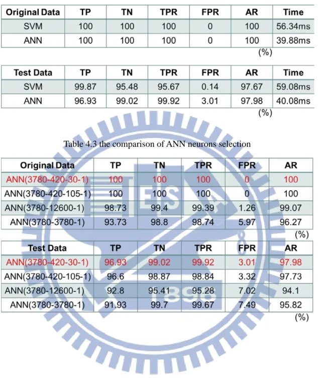
In this thesis, it adopts original data which includes 1500 positive data and 1328 negative data to test the performance of human shape recognition. Similarly, it also adopts same amount of positive test data and negative test data for the performance test. The performance and average executing time of two approaches are shown in Table 4.2, including TP, TN, TPR, FPR, AR, average executing time. Besides, the comparison of ANN neurons selection is shown in Table 4.3. In Table 4.3, the performance of two hidden layers is better than the performance of one hidden layer since original data in two hidden layers could be classified perfectly and test data in two hidden layers have higher AR. Hence, the system uses two hidden layers to establish ANN classifier. In Table 4.2, the classifiers of SVM and ANN have the similar AR, but have obviously different executing time. In system execution, ANN classifier has higher executing speed than SVM classifier. However, the training of ANN classifier spends much more time than the training of SVM classifier. Therefore, each of SVM classifier and ANN classifier has its advantages and disadvantages.

TP

FP

FN

TN

1

0

Actual Condition

1

0

Test

Result

Table 4.2 the performance and average executing time of two approaches

Table 4.3 the comparison of ANN neurons selection

4.4 Motionless Human Checking

In this section, taking Fig-4.6 as an example, there are three continue frames in the situation which first frame is human still with motion, second frame is human without motion and third frame is human without motion as well. In Fig-4.6(a), human with motion has been recognized successfully, and human without motion is

also recognized in Fig-4.6(b) and Fig-4.6(c). As a result, motionless human could be considered as new ROI in the next frame and successfully recognized by feature extraction and human shape recognition as well.

(a)

(b)

(c)