容積陰影的時間適應性取樣演算法

國立交通大學

多媒體工程研究所

碩 士 論 文

容積陰影的時間適應性取樣演算法

Temporally Adaptive Sampling for Volumetric Shadow Algorithms

研 究 生： 林相宇

指導教授： 施仁忠 教授

張勤振 教授

容積陰影的時間適應性取樣演算法

Temporally Adaptive Sampling for Volumetric Shadow Algorithms

研究生： 林相宇

Student:

Hsiang-Yu Lin

指導教授： 施仁忠

教授

Advisor: Dr. Zen-Chung Shih

張勤振

教授

Dr. Chin-Chen Chang

國 立 交 通 大 學

多 媒 體 工 程 研 究 所

碩 士 論 文

A Thesis

Submitted to Institute of Multimedia Engineering College of Computer Science

National Chiao Tung University in partial Fulfillment of the requirements

for the Degree of Master

in

Computer Science

June 2012

Hsinchu, Taiwan, Republic of China

I

容積陰影的時間適應性取樣演算法

研究生: 林相宇

指導教授

施仁忠 教授

張勤振

教授

國立交通大學多媒體工程研究所

摘 要

II

Temporally Adaptive Sampling for Volumetric Shadow Algorithms

Student: Hsiang-Yu Lin

Advisor: Dr. Zen-Chung Shih

Dr. Chin-Chen Chang

Institute of Multimedia Engineering

National Chiao-Tung University

ABSTRACT

Scattering in participating media generates volumetric lighting effects known as crepuscular or god rays. Such effects greatly enhance the realism in virtual scenes. However, they are inherently costly as scattering occurs at every point in sampling space and thus it needs costly integration of the light scattered towards the observer. This is often done using ray marching which is too expensive for each pixel on the screen for interactive applications. We propose a method to reduce samples in time domain, which means that we can reuse the information from the previous frame. In dynamic scenes, to decide pixels that can not be reused, we create shadow volumes of moving objects and rasterize them. Using a stencil buffer to maintain the information of screen pixels needs to recompute or just use the old information. We show that our method is simple to implement and yields the same quality but with a specific speedup.

III

Acknowledgements

First of all, I would like to express my sincere gratitude to my advisor, Prof. Zen-Chung Shih and Prof. Chin-Chen Chang for their guidance and patience. Without their encouragement, I would not complete this thesis. Also thank to Prof. Yu-Ting Tsai and all the members in Computer Graphics and Virtual Reality Laboratory for their reinforcement and suggestion. Thanks for those people who have supported me during these days. Finally, I want to dedicate the achievement of this work to my family and the natural beauty around daily life.

IV

Content

Chapter 2 Related Works ... 5

2.1 Scattering Effect………...……….5

2.2 Visibility Query………...…………5

2.3 Epipolar Sampling……….………..…………6

Chapter 3 Background Knowledge ... 8

3.1 Participating Media……….………8

3.2 Volumetric Shadows……….…10

3.3 Hybrid Ray Marching and Shadow Volume……….…11

Chapter 4 The Algorithm………..…12

4.1 Shadow Volumes of Moving Objects………...……….………12

4.2 Dynamic Mask………..………….………...14

Chapter 5 Implementation Detail………..…….…...19

5.1 Stencil Mask Setting………...19

5.2 Combine Temporal Frame………..………20

Chapter 6 Results and Discussion ... 23

Chapter 7 Conclusions and Future Work ... 31

V

List of Figures

Figure 1.1: Scattering effect enhance realism………….………2

Figure 1.2: Flow chart of our proposed algorithm………..…..…3

Figure 1.3: Temporal adaptive sampling of scattering effect frame…………...………4

Figure 3.1: Symbols along a viewing ray [23]………....……9

Figure 3.2: Lit segments………...……….……..9

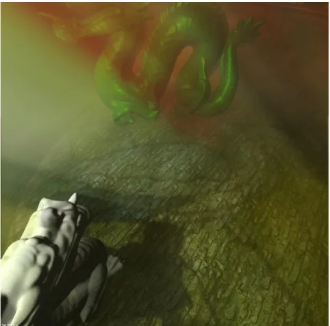
Figure 4.1: The whole scene with scattering effects…..……….……..14

Figure 4.2 The dynamic mask……….….….14

Figure 4.3: Generate shadow volumes……….……….16

Figure 4.4: Generate a stencil mask………17

Figure 4.5: Combine results………..…………...……….…18

Figure 5.1: Reused frame number……….…21

Figure 5.2: Reused frame number and frame rate……….……21

Figure 5.3: Artifact when reused frame number exceeds a number………..……..22

Figure 6.1: Scene “dragon”……….…..25

Figure 6.2: Scene “donuts & dragon”……….…..26

Figure 6.3: Scene “bunny”.………...……….……….………..27

Figure 6.4: Scene “buddha”………..28

Figure 6.5: Scene “bigScene”……….……..29

VI

List of Tables

1

Chapter 1

Introduction

1.1 Motivation

Global illumination effects, for example, indirect lighting, soft shadows, caustics, or scattering heavily enhance the realism of rendered virtual scenes. However, they need a lot of computational cost. It is challenging for real time applications. In particular, effects which involve participating media are complicated. Considering about participating media implicates that not only surfaces are concerned, but also it requires the evaluation of the scattering radiance at each point in space. Some simplifying assumptions, such as the limitation to single-scattered light only, are often made to ease computation cost. Fortunately, in many cases, these effects suffice to produce convincing results.

We inherit this direction and concentrate on single-scattering effects (see Figure 1.1). Ray marching [20] is usually used, which needs to integrate inscattered light along a ray emanating from the camera. Consequently, the computation cost scales with the number of rays and samples along the ray. The previous work [23] uses down sampling to reduce the number of rays, and restricts ray marching regions to lit segments (shadowed regions do not contribute). Another approach [7] uses irregular sampling and interpolates to reduce number of rays.

In this thesis, we show that several screen information can be reused in dynamic scenes, and thus we can reduce number of rays reusing the results from the previous frame. Therefore, the main speedup is coming from reusing, which means that we have to determine pixels on

2

the screen whether they are needed to be updated or not. We focus on moving objects that are changed frame by frame and we make a stencil buffer to mask pixels that are not reusable by rasterizing these objects. But this is not enough because participating media is involved. are also consider the shadow volume of these objects. This temporally adaptive sampling strategy can be combined into exist rendering systems without obviously quality loss and yields a definite speedup.

1.2 System Overview

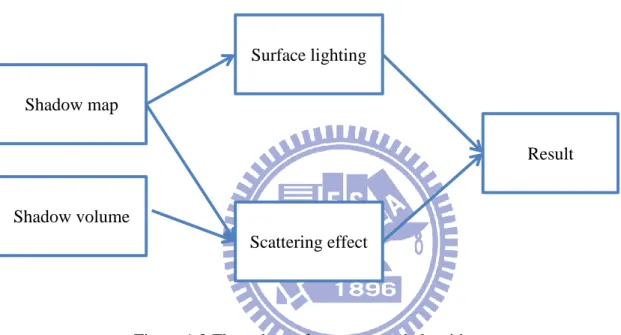
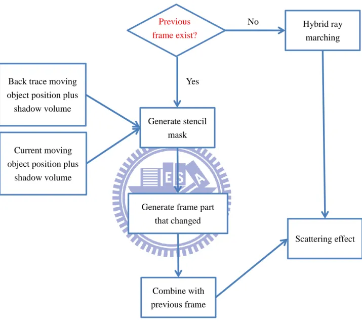
Figure 1.2 shows the flow chart that includes two parts. The first part is surface lighting that we can do it quickly with openGL library. The second part is about scattering effects that consider about participating media. Figure 1.3 focuses on scattering lighting and shows the procedure of our proposed temporally adaptive sampling. First, we check whether that full quad of screen frame exists or not. If it does not exist, we compute it with the original

3

rendering technique. With the previous frame, we can focus on finding out which regions of the frame are needed to recompute due to moving objects. We first generate a stencil mask and use it to adopt ray marching. Finally, we combine the previous frame with the frame generated using the stencil mask.

1.3 Thesis Organization

The rest parts of this thesis are structured in the following manner. First, in Chapter 2, we will review some related works in volumetric shadows and scattering. Then, Chapter 3 introduces some background knowledge that is involved or used in this thesis. Chapter 4 describes the major method and algorithm used in our temporally adaptive sampling for volumetric shadow. Chapter 5 describes some implementation details and Chapter 6 shows the results of our algorithm and makes some discussion. Finally, in Chapter 7, we give some conclusions and some future works.

Shadow volume Shadow map

Surface lighting

Result

Scattering effect

4 No Previous frame exist? Hybrid ray marching

Back trace moving object position plus

shadow volume

Current moving object position plus

shadow volume

Generate stencil mask

Generate frame part that changed

Combine with previous frame

Scattering effect

Figure 1.3 Temporal adaptive sampling of scattering effect Yes

5

Chapter 2

Related Works

2.1 Scattering Effect

Traditional method for computing volumetric shadows with single scattering is ray marching. For each pixel on the screen, a ray is cast from the eye. And approximated radiance is computed by sampling along the ray. If the point is occluded from the light, it is discounted from the integral. The ray terminates once it hits an object’s surface.

Several research approaches work on solving single-scattering integral semi-analytically [18,21], but these studies ignore shadowing, which is often needed for realism and is the effect we focus on. Other methods like volumetric photon mapping [11,12] and line space gathering [22] dedicate to more difficult scattering issues, such as volumetric caustics or multiple scattering. These problems mentioned are far from real time on complex scenes.

Max [14] computed the single-scattering integral by searching the lit parts on every ray using shadow volumes intersected with epipolar slices. Then analytically compute the integral on each lit part.

2.2 Visibility Query

Wyman and Ramsey [23] restricted sample regions with shadow volumes, and used a shadow map to further determine visibility inside the region. Hu et al. [9] used Wyman and Ramsey’s method [23] in their algorithm for interactive volumetric caustics. It works for simple occlusion, but it is slow when visibility boundaries become complex.

6

The algorithm of Billeter et al. [2] generates the shadow volume extruded from a shadow map and computes the lit segments with a GPU rasterizer. It performs well for low-resolution shadow maps. This means that the performance is dependent on shadow map resolution. If a 40962 shadow map is applied, the performance will be slow down as predicted.

2.3 Epipolar Sampling

Volumetric shadow problems can be simplified using epipolar geometry [7,14]. Max [14] updated the hidden segments of view rays along epipolar planes. Then he computed scattering integrals of lit segments analytically, implying that complexity of the visibility function is proportional to integration cost. The shadow volume algorithm is dependent on scene complexity.

Recently, Engelhardt and Dachsbacher [7] noticed that values of the scattering integral vary smoothly along epipolar plane lines in most cases except at depth discontinuities. They sampled more at discontinuities occurred due to occlusion in image space. A Z-buffer is used for detecting, and visibility is queried from the shadow map. Compared to ray marching, this sampling strategy can speed up for most cases.

Incremental integration method is proposed by Baran et al [1]. They used epipolar rectification to reduce computation of scattering integral and accelerate this computation with a partial sum tree. This method is very fast on the CPU, but hard to implement to GPU due to incremental traversal of camera rays in specified order. For utilizing GPU parallelism, Chen et al. [4] used a 1D min-max data structure to avoid dependence between camera rays. They do not have to do camera rectification and avoid processing twice as many as camera rays. Their

7

results show that their approach can speed up and slightly obtain better quality. Wyman and Ramsey [24] also utilized epipolar space with voxelization. They reduced visibility query cost by voxelizing the scene into a binary, epipolar space grid. A fast parallel scan is then used to identify shadowed voxels. Once identified, a texture can be built according to this voxelized shadow volumes. Then, 128 visibility samples along the eye ray can be done with a single texture fetch.

Engelhardt and Dachsbacher [7] reached a definite speedup. However, there are some improvements by reusing temporal information. Our method focuses on this part, and shows a slighter speedup with almost the same quality.

8

Chapter 3

Background Knowledge

3.1 Participating Media

Considering particles in the air, intensity is modified through emission, absorption, in-scattering, and out-scattering. The discussion of these phenomena is not in the scope of this thesis. We only focus on discussing homogeneous single-scattering media.

The following equation based on the discussion by Nishita et al. [17] is used in our model:

L = L

+L

= L

e

+

∫ k

ρ(α)

e

_{dx , (1)}

where two terms Lattn and Lsctr represent attenuated light reflected from surface point s and

additional light contributed by in-scattering along the viewing ray, respectively. The radiance reflected from s towards the eye is marked as Ls, light’s emitted radiance is I0, the distance

from the eye to s is ds, and the distance from the light to an arbitrary point on the viewing ray

at distance x from the eye is d, as illustrated in Figure 3.1. Absorption and scattering coefficients are ka and ks, respectively, and phase function is ρ(α).

9

Figure 3.1 Symbols along a viewing ray. [23]

Figure 3.2 (Left) Ignoring segments with no contribution, we compute only segments from eye to d1, d2 to d3, and d4 to d5. (Right) [23]

10

3.2 Volumetric Shadows

We can render volumetric shadows by using shadow volumes [3,15]. Regions between shadow quads are the key points, because they have I0 = 0 and thus make no contribution to

the integral in Equation 1. We can compute each illuminated interval by splitting the integral of the following equation and Figure 3.2 (left) shows an illustration.

L

=k

I

[∫ f(x)dx+ ∫ f(x)dx+

∫ f(x)dx

], (2)

where f(x)=p(𝛼)_d2 e-(ka+ks)(d+x). According to [21], every illuminated segment along the viewing

ray can be simplified to two lookup functions. Front facing polygons and back facing polygons are positive and negative contributions, respectively.

However, some shadow polygons are unnecessary to the computation. As shown in Figure 3.2, parts of shadow polygons overlap, and certain polygons are valid in certain regions. Solving these problems requires repeated depth peeling in order to sort shadow quads [3]. It is costly because even for simple scenes, it needs numerous passes. Moreover, rendering shadow quads spends significant fill rate for stencil shadow pass.

Other approaches such as volume rendering technique [6], or ray marching [13] have to take care about shadow boundaries, which take additional work.

Therefore we adopt a hybrid method proposed by Wyman and Ramsey [23], which uses ray marching to eliminate the soring requirement of shadow volume approaches and only ray marching in regions where shadows exist. They used shadow volumes to distinguish the shadow regions of each ray.

11

3.3 Hybrid Ray Marching and Shadow Volume

Instead of sampling all the points of a viewing ray, this hybrid method samples in certain regions. The basic idea can be described as follows: Render shadow volumes from light direction, store the distance between front-most polygons and also store distance between back-most polygons. These distances will help us determine regions where shadows exist. As shown in Figure 3.2, if samples are between eye and d1, d4 and d5, they are lit. For the lit

segments, use the air-light model [21] directly. Other samples which in the regions between front-most and back-most seen from eyes are determined visibility by the shadow map.

Rendering procedure is shown as follows: 1. Render a shadow map.

2. Store distances between shadow polygons and the eye (front-most and back-most only).

3. Render the scene without shadows.

4. Render single-scattering effects and pixels encountered no shadow quads are computed by the air-light model [21] directly. The rest pixels of each lit segment are determined using the shadow map, and the contribution can be computed by the air-light model.

5. Combine Lattn and Lsctr as results.

This ray marching technique can reach a definite speedup compared to the traditional ray marching. However, ray marching with participating media still consumes a lot of performance. Therefore, we propose a temporal sampling to reduce samples in dynamic scenes. Our basic idea is to reuse information that is not changed from the previous frame. More details are introduced in Chapter 4.

12

Chapter 4

The Algorithm

We develop a novel real-time sampling algorithm for dynamic scenes with moving objects. Acceleration is coming from reducing number of samples for ray marching. The concept of temporal sampling is reusing. We consider what is changed in the current frame. For the part that is not changed, we can directly use the information from the previous frame. Effects we care about are god rays or crepuscular rays that generated by considering participating media. Because of participating media, samples in the scene volume influence the results of ray marching. This is important for deciding pixels whether they are changed or not. If visibility of samples in the scene volume along a viewing ray is changed, this ray should be computed. Otherwise we directly use the ray marching results of the previous frame. Thus a stencil mask is built for classifying pixels. This mask is made from considering the shadow volume of moving objects and moving objects. We need the current positions and the previous positions of moving objects to generate such a mask. We will describe more details in the following sections.

4.1 Shadow Volumes of Moving Objects

We generate a shadow volume of moving objects because the visibility of particles within the shadow volume will be changed. Therefore, ray marching results of the pixels will be different since we consider participating media. Therefore, the shadow volume of moving objects is an important part to indicate changed pixels of the screen.

Assume that we know what objects are moved. We generate the shadow volume within a shader. First, silhouettes of the moving object are generated. Then two more vertices for each

13

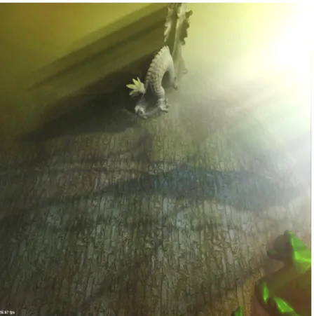
silhouette are added to produce shadow polygons. Figure 4.1 shows the whole scene and the moving object is the dragon. Figure 4.2 shows the stencil mask generated from the object and the shadow volume. Light is in the left of the scene. The mask marks the changed results of ray marching which can not be reused. The results of ray marching of other parts remain the same as the previous frame.

4.2 Dynamic Mask

The stencil mask of current moving objects is not enough for specifying all changed pixels, because it only includes samples that are changed from visible to invisible. We should also consider visibility of samples that are changed from invisible to visible. This usually happens in the shadow volume of moving objects of the previous frame.

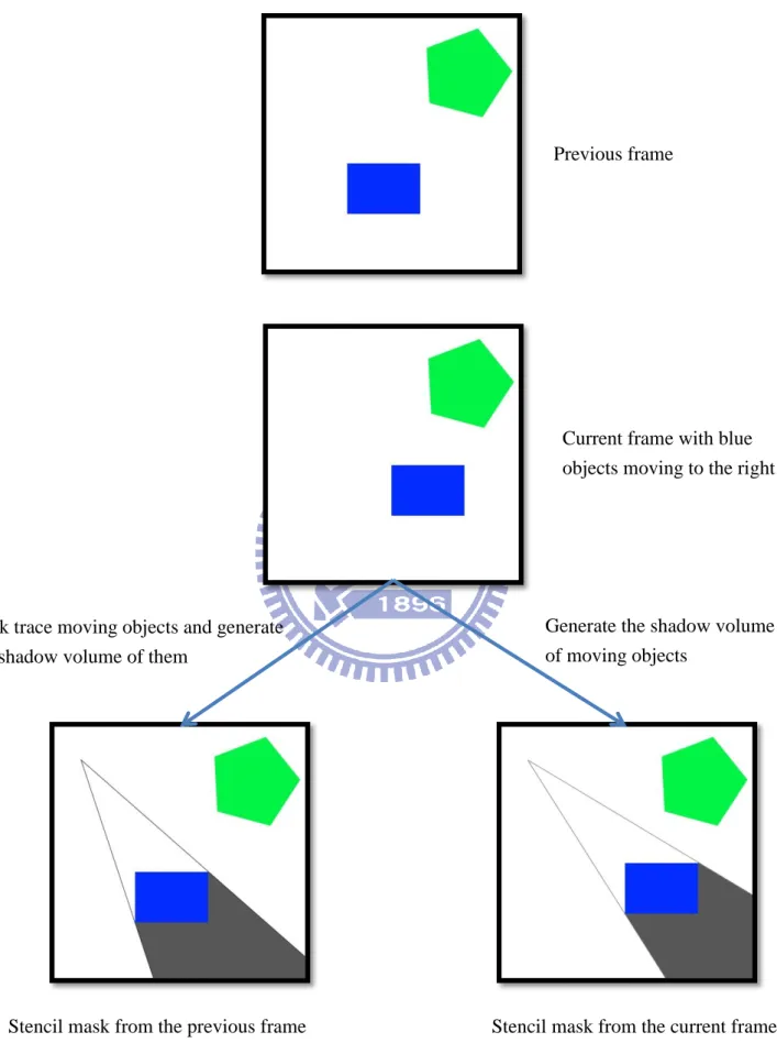
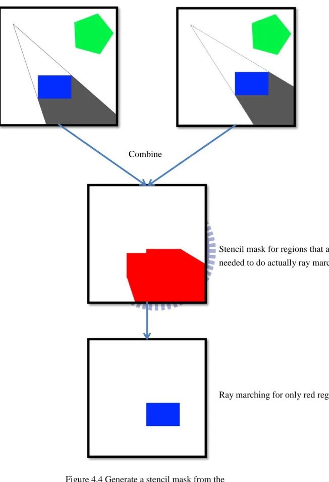
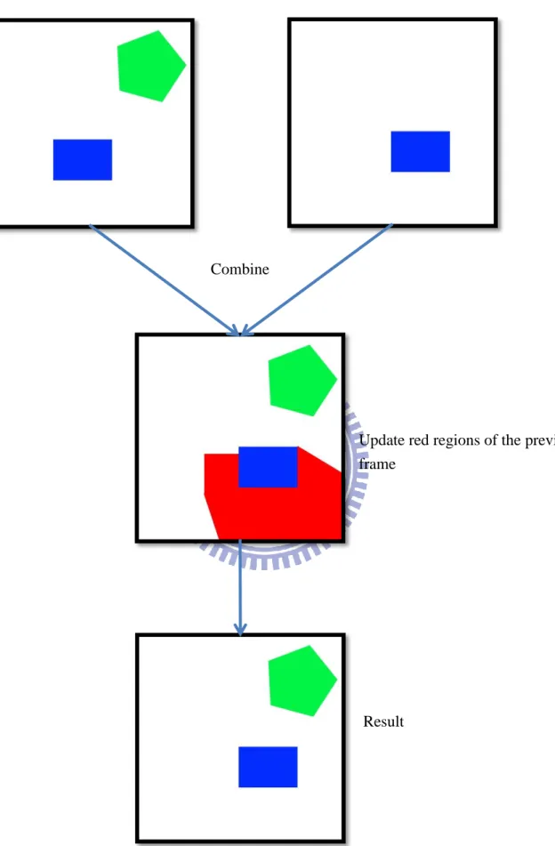
Both the previous and current shadow volumes of moving objects are considered. Actually, we consider all shadow volumes of moving objects from the previous frame to the current frame. But since the time step between two frames is very small, the previous and current shadow volumes of moving objects can approximately cover all pixels that we want to mask. Figure 4.3 shows that we back trace positions of moving objects of the previous frame and generate shadow volumes of them, and do the same procedure for the current frame. Notice that there is no need to compute all pixels in the current frame. We show all the scenes just for helping understanding. Figure 4.4 shows that we combine two stencil masks from Figure 4.3. This combined mask help indicate which pixels are needed to ray marching due to movements of objects. We then use it to compute pixels that are marked changed. Figure 4.5 shows that we combine the results from the previous frame and the current frame by updating red regions from the previous frame.

14

Figure 4.1 The whole scene with scattering effects

15

Experiments show this approximate strategy can handle all changed pixels expect the frame rate is slow. In some special cases, such as scenes with a lot of moving objects, scenes with sophisticated objects or moving objects covering almost all screen pixels, our algorithm can not perform well. The frame rates of these special cases are slow. Difference will become a little more obvious in these cases. Totally, the quality can remain the same. We capture the frames produced with our algorithm and the hybrid ray marching. The difference image of these two frames shows zeroes for all pixels if the frame rate is high. We notice that types of motion also affect the dynamic stencil mask. A linear motion will not lose pixels in general, but a rotate motion may leave some pixels out of the mask. We can handle this situation by updating whole frames with a definite number of frames. We call this number the reused frame number, and give more details in the following chapter. Using a large time step to build the mask is also a solution, but it will cause much overhead since more shadow volumes are needed.

16

Stencil mask from the previous frame Stencil mask from the current frame Previous frame

Current frame with blue objects moving to the right

Back trace moving objects and generate the shadow volume of them

Generate the shadow volume of moving objects

Figure 4.3 Generate shadow volumes of objects of the previous frame and current frame

17 Combine

Figure 4.4 Generate a stencil mask from the generated shadow volume

Stencil mask for regions that are needed to do actually ray marching

18 Combine

Update red regions of the previous frame

Result

Figure 4.5 Combine results from the previous frame and current frame

19

Chapter 5

Implementation Detail

We develop our algorithm based on openGL and GLSL. Most jobs are stored as textures from different rendering passes and combined to get the rendering effects. Our temporally adaptive sampling technique dedicates to reducing samples by reusing ray marching results from the precious frame. Therefore, at least two rendering passes are added to the rendering system. One is for building a stencil mask and another is for combining the reusable parts and the actually recomputed parts.

5.1 Stencil Mask Setting

As Figure 4.4 (red parts) shows, our mask includes not only rasterization of moving objects and the shadow volume, but also the parts in the previous frame. This is done with stencil operations and stencil function sets. Stencil operations specify actions when stencil or depth tests pass or not. When building this mask, we do not need to consider about depth information and depth test is disabled. Stencil functions specify stencil tests that decide whether pixels pass the mask or not. During the rendering pass, all the changed parts of the screen will be set to non-zero in the stencil mask. Therefore we use GL_NOTEQUAL parameters to distinguish pixels which need ray marching.

After setting stencil operations and stencil functions, a shader is performed to generate a shadow volume of moving objects. We perform this shader twice separately for the current positions of moving objects and the same moving objects but with positions of the previous frame. Pixels with different ray marching results due to moving objects are then marked as non-zeroes in the stencil mask.

20

Note that as above mentioned, we store different rendering passes as different textures. We use off-screen rendering techniques to do so. Frame buffer object of openGL is convenient to do this, but it is only a manager of memory to help us control off-screen render. Each render buffer should be created before it is used, such as depth buffer, stencil buffer and so on.

5.2 Combine Temporal Frame

Once we finish building the stencil mask, a texture with results of the changed parts can be generated, as shown in Figure 4.2. We need to compute the whole scene at least once and imagine it as background. Then a shader is applied to combine this background texture and the current changed part of the texture. Actually it is not necessary to process every pixel. We just take the background texture as render targets and process only pixels that are within the stencil mask.

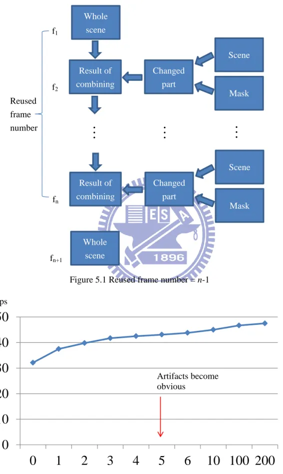
The reused frame number should be taken into account with this combined strategy. We compute the whole scene per this reused frame number (see Figure 5.1). Assume the camera is fixed, we only need to compute the background texture once. We can get the best speedup in this case. That is, assume that we generate a background texture where whole pixels are considered taking 200ms and a texture with only pixels covered by stencil mask taking 50ms. If we reuse the more frames, the closer to 50ms per frame we can reach (see Figure 5.2). In our case, we set the reused frame number to 3, because the stencil mask sometimes can not fully cover the regions that we want. If we set the reused frame number to more than a definite number, some unwanted colors would be accumulated and it produces obvious artifacts, as shown in Figure 5.3. Fortunately, 3 reused frames can achieve almost 70% of the best speed.

21

0

10

20

30

40

50

0

1

2

3

4

5

6

10 100 200

…

…

…

Figure 5.1 Reused frame number = n-1

Whole scene f1 Result of combining Changed part Scene Mask f2 Result of combining Changed part Scene Mask fn Whole scene fn+1 Reused frame number Reused frame number Figure 5.2 Relation between reused frame number

22

Figure 5.3 Artifacts when reused frame number exceeds a number. (a) Normal (b) with artifacts

(a)

23

Chapter 6

Results and Discussion

We run our algorithm on a PC with 3.33 GHz Core™ i7 CPU and 8.0GB of memory. The graphics card is an NVDIA GeForce GTX 295. Table 6.1 shows the running time of our temporally adaptive sampling and of the hybrid ray marching. In most scenes, such as dragon, bunny and buddha, we can reach a definite speedup with almost the same quality. However, the speedup is coming from reusing ray marching results from the previous frame. Therefore, performance is directly proportional to moving objects and the shadow volume of the moving objects covering pixels. Moving objects of scenes “donuts & dragon” cover almost the whole scene, as shown as Figure 6.2. Therefore, there is no speedup due to reuse rare pixels. Figure 6.3 and Figure 6.4 gain more speedups due to less pixels are changed, which means that we reuse most parts of the previous frame. Figure 6.5 shows the scene bigScene. The speedup is not so obvious due to more moving objects. We generate the shadow volume of moving objects so that more objects will produce more overhead. Besides, the big dragon covers almost fifty percent of the screen. Figure 6.6 shows less speedup to scene yeahRight which is because of sophisticated model and the overhead of building shadow volumes making frame rate increasement limited.

There are three factors for affecting speedups: the number of moving objects, the stencil mask occupying pixels and the complexity of moving objects. All these factors exist when the performance of our algorithms becomes slow. As shown in Table 6.1, scene donuts & dragon is slow because of the number of moving objects and the stencil mask occupying pixels. Scene bigScene is due to the number of moving objects and scene yeahRight is influenced by the complexity of moving objects. Generate a shadow volume for our stencil mask is an

24

important reason to these factors. We could improve this condition by a more efficient method to generate shadow volume of moving objects.

Scene Our approach (fps) Hybrid ray marching (fps)

dragon 46.08 35.24

bunny 59.93 44.73

buddha 58.76 41.63

donuts & dragon 41.32 43.31

bigScene 31.54 28.78

yeahRight 29.34 26.75

25

Figure 6.1 Scene “dragon”.

(a) 46.08 fps by our algorithm, (b) 35.24 fps by hybrid ray marching

(a)

26

(a)

Figure 6.2 Scene “donuts & dragon”.

(a) 41.32 fps by our algorithm, (b) 43.31 fps by hybrid ray marching (b)

27

Figure 6.3 Scene “bunny”.

(a) 59.93 fps by our algorithm, (b) 44.73fps by hybrid ray marching (a)

28

Figure 6.4 Scene “buddha”.

(a) 58.76 fps by our algorithm, (b) 41.63 fps by hybrid ray marching (a)

29

Figure 6.5 Scene “bigScene”.

(a) 31.54 fps by our algorithm, (b) 28.78 fps by hybrid ray marching (a)

30

Figure 6.6 Scene “yeahRight”.

(a) 29.34 fps by our algorithm, (b) 26.75 fps by hybrid ray marching (a)

31

Chapter 7

Conclusions and Future Work

In this thesis, we propose a temporally adaptive sampling method and actually reduce sample numbers needed. We achieve a definite speedup compared to [23] and we believe that more speedups can be reached if this method is adopted to ray marching techniques with better quality, because down-sampling has been done with the proposed rendering techniques. Besides, this method can be easily integrated to other rendering techniques due to two rendering passes are needed only.

There are some limitations in our method. If moving objects and their shadow volumes cover too many pixels of the screen, speedup will be limited. And if the camera is keeping moving, there will be no pixels reusable. Therefore, we show a little speedup or no speedup in these cases.

In the future, we want to generate the stencil mask more efficiently. Save the stencil mask of the objects of the previous frame and adopt it in the current frame when they are detected moving, since we need to generate shadow volumes of the objects to compute ray marching results. Another feasible method is to generate a shadow volume from a shadow map. Besides, a dynamic detection of changed parts of the stencil mask can be applied to decide whether using this sampling method or not. If moving objects and their shadow volumes cover over a definite percentage of the screen, we do not use this method.

32

References

[1] BARAN, I., CHEN, J., RAGAN-KELLEY, J., DURAND, F., AND LEHTINEN, J. 2010. A hierarchical volumetric shadow algorithm for single scattering. ACM Transactions on

Graphics 29, 5.

[2] BILLETER, M., SINTORN, E., AND ASSARSSON, U. 2010. Real time volumetric shadows using polygonal light volumes. In Proc. High Performance Graphics 2010. [3] BIRI, V., ARQUES, D., AND MICHELIN, S. 2006. Real time rendering of atmospheric

scattering and volumetric shadows. Journal of WSCG, 14:65-72.

[4] CHEN, J., BARAN, I., DURAND, F., AND JAROSZ, W. 2011. Real-Time volumetric shadows using 1D min-max mipmaps. In ACM Symposium on Interactive 3D Graphics

and Games.

[5] DOBASHI, Y., YAMAMOTO, T., AND NISHITA, T. 2000. Interactive rendering method for displaying shafts of light. In Proc. Pacific Graphics, IEEE Computer Society, Washington, DC, USA, 31.

[6] DOBASHI, Y., YAMAMOTO, T., AND NISHITA, T. 2002. Interactive rendering of atmospheric scattering effects using graphics hardware. In Proc. Graphics hardware, 99–107.

[7] ENGELHARDT, T., AND DACHSBACHER, C. 2010. Epipolar sampling for shadows and crepuscular rays in participating media with single scattering. In Proc. 2010 ACM

SIGGRAPH symposium on Interactive 3D Graphics and Games, ACM, 119–125.

[8] HACHISUKA, T., JAROSZ, W., WEISTROFFER, R, P., DALE, K., HUMPHREYS, G., ZWICKER, M., AND JENSEN, H, W. 2008. Multidimensional adaptive sampling and reconstruction for ray tracing. ACM Transactions on Graphics 27, 3.

[9] HU, W., DONG, Z., IHRKE, I., GROSCH, T., YUAN, G., AND SEIDEL, H.-P. 2010. Interactive volume caustics in single-scattering media. In I3D ’10: Proceedings of the

33

2010 symposium on Interactive 3D graphics and games, ACM, 109–117.

[10] IMAGIRE, T., JOHAN, H., TAMURA, N., AND NISHITA, T. 2007. Anti-aliased and real-time rendering of scenes with light scattering effects. The Visual Computer 23, 9–11 (Sept.), 935–944.

[11] JAROSZ, W., ZWICKER, M., AND JENSEN, H. W. 2008. The beam radiance estimate for volumetric photon mapping. Computer Graphics Forum 27, 2 (Apr.), 557–566. [12] JENSEN, H. W., AND CHRISTENSEN, P. H. 1998. Efficient simulation of light

transport in scenes with participating media using photon maps. In Proc. SIGGRAPH 98, 311–320.

[13] LEFEBVRE, S. AND GUY, S. 2002. Volumetric lighting and shadowing. http://www.aracknea-core.com/sylefeb/page.php?c=Shaders.

[14] MAX, N. L. 1986. Atmospheric illumination and shadows. In Computer Graphics (Proc.

SIGGRAPH ’86), ACM, New York, NY, USA, 117–124.

[15] MECH, R. 2001. Hardware-accelerated real-time rendering of gaseous phenomena.

Journal of Graphics Tools, 6(3):1-16.

[16] MITCHELL, K. 2008. Volumetric light scattering as a post-process. In GPU Gems 3, Addison-Wesley.

[17] NISHITA, T., MIYAWAKI, Y. AND NAKAMAE, E. 1987. A shading model for atmospheric scattering considering luminous distribution of light sources. In Proceedings

of SIGGRAPH, pages 303–310.

[18] PEGORARO, V., AND PARKER, S. 2009. An analytical solution to single scattering in homogeneous participating media. Computer Graphics Forum 28, 2.

[19] PEGORARO, V., SCHOTT, M., AND PARKER, S. G. 2010. A closed-form solution to single scattering for general phase functions and light distributions. Computer Graphics

Forum 29, 4, 1365–1374.

34

to Implementation. Morgan Kaufmann

[21] SUN, B., RAMAMOORTHI, R., NARASIMHAN, S., AND NAYAR, S. 2005. A practical analytic single scattering model for real time rendering. ACM Trans. Graph. 24, 3.

[22] SUN, X., ZHOU, K., LIN, S., AND GUO, B. 2010. Line space gathering for single scattering in large scenes. ACM Trans. Graph. 29, 4.

[23] WYMAN, C., AND RAMSEY, S. 2008. Interactive volumetric shadows in participating media with single-scattering. In Proc. IEEE Symposium on Interactive Ray Tracing, 87-92.

[24] WYMAN, C. 2011. Voxelized shadow volumes. ACM/EG Symposium on High