A Study on Parity Checks in Stream Cipher Correlation Attacks

全文

(1)A Study on Parity Checks in Stream Cipher Correlation Attacks Jun-Chu Hong , Wen-Nung Tsai , Rong-Jaye Chen Department of Computer Science and Information Engineering, National Chiao Tung University, Hsinchu, Taiwan, R.O.C. Email: {hongjc, tsaiwn, rjchen} @csie.nctu.edu.tw memory, when a block cipher system does not. The essential difference between block and stream ciphers is the usage of memory as is shown in Figure 1.1.. ABSTRACT The commonest stream cipher system uses a keystream generator which consists of several LFSRs combined by a combining function. If there exists a measure of correlation between the output sequence of the keystream generator and an arbitrary LFSR, the initial state of the LFSR can be reconstructed by a correlation attack, that is, the partial key in the LFSR is determined. W. Meier and O. Staffelbach proposed a correlation attack method using parity check equations.. K. c. device with Memoryless device. sL. sj c. Figure 1.1.. internal memory. c j = E z j (s j ). c = E K (s ). In this paper, we discuss the algorithm and its constraints, and then propose some improvements: computing more low-weight parity check equations, accounting the precise number of relations of each digit, and solving the system of linear independent equations from digits instead of calculating the whole output sequence and the initial state of the LFSR from the relations among the digits.. zj =. f j (K ,σ j ). The difference between block and stream ciphers. Obviously, we can think of a block cipher as a special case of a stream cipher where the keystream is constant: zj = K. In this paper, we focus on stream cipher systems and correlation attacks on stream ciphers.. 1.Introduction. There are two different approaches to stream encryption: synchronous methods and self-synchronous methods [16][17]. In a synchronous stream cipher, as shown in Figure 1.2, the next state depends only on the previous state and not on the input so that the succession of states is independent of the message stream. The keystream is therefore generated independently of the message stream. Thus, if a ciphertext character is lost during transmission, the sender and receiver must resynchronize their generators before they proceed further.. In cryptography, there are two basic types of symmetric encryption/decryption algorithms: block ciphers and stream ciphers [14][15]. Block ciphers operate on blocks of plaintext and ciphertext. The same plaintext block will be always encrypted to the same ciphertext block, using the same key. Stream ciphers operate on streams of plaintext and ciphertext one bit or byte at a time. The same plaintext bit or byte will be encrypted to a different bit or byte every time it is encrypted. That is, for a plaintext string s = s1s2 … s L in a block cipher system, the ciphertext string c is obtained as follows.. K. c = c1c2 …cL = EK ( s1 ) EK ( s2 ) … EK ( s L ) And for a plaintext string s = s1s2 … in a stream cipher system, the ciphertext string c is obtained as follows.. c = c1c2 … = Ez1 (s1 ) Ez2 (s2 )…. K. s1. ∞. where the keystream ( or called ‘running key’ ) z is z1 z 2 … , the actual key is K, and the state of the encryption device is σj which may be dependent on K, σ th j-1 and sj-1, and the function fj is used to generate zj ( the j element of the keystream ) such that. K. Secure. Keystream. Keystream. Generator. Generator. zj sj. c E z j (s j ). z j = f j (K ,σ j ). Figure 1.2. Thus a stream cipher system keeps a stateσ j in the 1. zj sj D z j (c j ) Synchronous stream ciphers. cj.

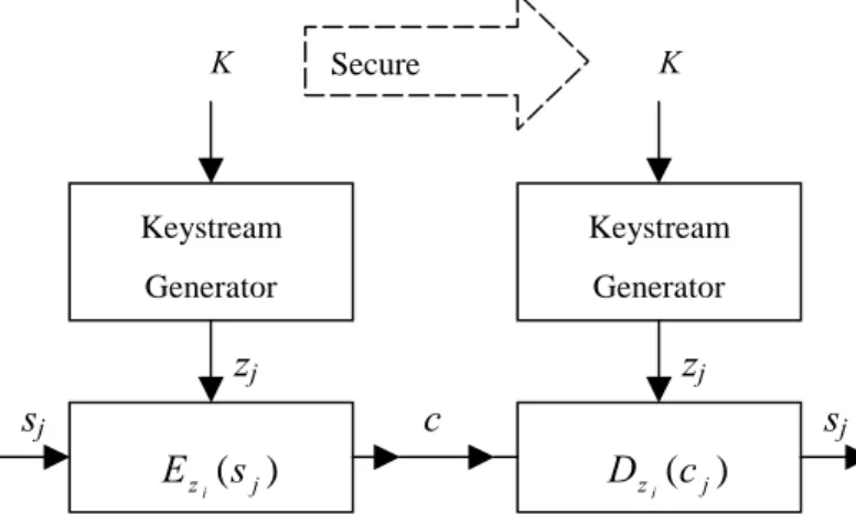
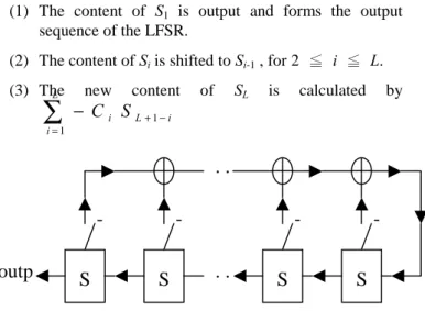
(2) K. Secure Channel. The keystream generator as a finite state machine consists of an output alphabet {zj} and a state set {σj} , together with two functions ( φ,Ψ ) and an initial state σ0. The next state function φ maps the current stateσj into a new stateσj+1 from the state set. The output function Ψ maps the current state σj into an output symbol zj from the output alphabet. The key K may determine the next state function φ and the output function Ψ as well as the initial stateσ0.. K. Keystream. Keystream. Generator. Generator. z. z. s. s E z j (s j ) Figure 1.3.. c. D z j (c j ). Self-synchronous stream ciphers. In a self-synchronous stream cipher, as shown in Figure 1.3, each keystream character is derived from a number n of preceding cipher characters. Thus, if a ciphertext character is lost or modified during the transmission, the error propagates forward for n characters, but the cipher resynchronizes itself after n correct ciphertext characters have been received. The algorithm that generates the keystream must be deterministic so that the stream can be reproduced for decipherment. One important kind of synchronous stream cipher is the additive synchronous stream ciphers, where the characters of the keystream are from an Abelian group (G,+) and the ciphertext character cj is the addition of the keystream character zj and plaintext stream character sj ( c j = s j + z j , s j = c j − z j and “-” means the inverse operation of “+” ) . In this thesis, we only discuss GF(2) , so the effects of “+” and “-” are both the same with XOR ( cj = sj + zj = sj − zj = sj ⊕ zj ) . Finite state machines are important mathematical objects for modeling electronic hardware. Furthermore, due to their recursive feature, finite state machines are convenient means for realizing infinite word-functions built over finite alphabets. Many keystream generators can be modeled by finite state machines. In a synchronous stream cipher, the keystream generator may be viewed as an autonomous finite state machine as depicted in Figure K 1.4.. φ. The major purpose of designing a keystream generator is to prevent from an attacker to predict the output sequence z. So the output sequence of the keystream generator should satisfy some cryptographic requirements such as long period, large linear complexity, good auto correlation, uniform pattern distribution ( randomness ) , and so on.. 2.Linear Feedback Shift Register based Stream Ciphers Linear Feedback Shift Registers ( LFSRs ) are the commonest components in stream cipher systems since they can generate binary sequences speedily. Figure 2.1 is the structure of a LFSR [16][17]. A linear feedback shift register of length L consists of L stages S1 ~ SL. Each stage stores one bit. During each unit of time, the following operations are executed : (1) The content of S1 is output and forms the output sequence of the LFSR. (2) The content of Si is shifted to Si-1 , for 2 ≦ i ≦ L. (3) The L. ∑. i =1. new. content. − C i S L +1− i. K Figure 1.4.. is. calculated. by. .. -. outp. S. Figure 2.1.. ... S. S. S. The Structure of a Linear Feedback Shift Register. L sequence s of So, the jth digit (bit) sj ( j > L ) of the output L s j = − Ci s j −i . In the LFSR can Lbe calculated from GF(2), s j = − Ci s j −i = Ci s j −i . i =1. ∑. σj. SL. of. Ψ. z. K. Keystream generators as autonomous finite state machines. ∑. i =1. c( x) = C L x L + C L −1 x. i =1. L −1. ∑. We use a polynomial. + ... + C1 x + 1 to record the. structure of the LFSR.. Definition. The initial content of the LFSR is called the initial state of the LFSR. In general, the initial state of the LFSR is the key or a part of the key of the stream cipher system. 2.

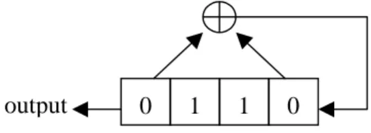
(3) r1 , r2 , ..., rt of 2m-1 . If any gi(x) = 1, then f(x) is not a Definition.. polynomial c( x) = C L x L + C L −1 x L −1 + ... + C1 x + 1 is called the connection polynomial of the LFSR. If the degree of c(x) is L, that is CL = 1, then the LFSR is nonsingular and the output sequence of the LFSR is periodic. Example.. The. Consider the LFSR in Figure 2.2.. The initial state of the LFSR of length 4 is 0, 1, 1, 0. The 4 connection polynomial is c( x ) = x + x + 1 . And for j > th 4, the j output digit of the LFSR is s j = s j −1 + s j − 4 . The output sequence is s = 0, 1, 1, 0, 0, 1, 0, 0, 0, 1, 1, 1, 0, 1, …, and is periodic with period 15 .. output Figure 2.2.. 0. 1. 1. 0. An illustration of a LFSR. primitive polynomial, else it is primitive.. Fact. If the connection polynomial of a LFSR of length L is a primitive polynomial of degree L, then each of the 2L-1 non-zero initial states of the non-singular LFSR generates an output sequence with period 2L-1 .. Since every m-sequence satisfies Golomb’s randomness postulates, it seems that we can take a LFSR with a primitive connection polynomial as a keystream generator. But it is not secure enough. In 1976, Abraham Lempel and Jacob Ziv [4] proposed to use the linear complexity of the keystream as a measure of the strength of a stream cipher system. Definition. The linear complexity of a finite binary sequence s of length n, denoted as Λ(s), is the length of the shortest LFSR that can generate a sequence having s as its first n digits. And Λ(s) = 0 if s is an empty string.. Theorem. The period of a sequence generated by a non-singular LFSR of length L is at most 2L-1 .. Since a LFSR of length L consists of L stages, the number of the contents of the LFSR is 2L. The next state of L-zeros is still all-zeros. So, a LFSR with all-zeros as its initial state can only generate a sequence of zeros, and the period is 1. If the initial state of a LFSR is not all-zeros, there are at most 2L-1 possible contents of the LFSR and the period of the change of the LFSR’s content is at most 2L-1. The output digit of a LFSR each step is dependent only on the previous state of the LFSR. So, the period of the output sequence of a non-singular LFSR of length L is at most 2L-1, too.. A sequence generated by a non-singular LFSR of length L is called a maximal sequence or m-sequence if its period is 2L-1, and the LFSR is called a maximal-length LFSR. Every m-sequence satisfies Golomb’s randomness postulates and is also a pn-sequence.. Fact. Suppose that the linear complexity of a binary sequence s is Λ(s). As long as we observe consecutive 2 Λ(s) digits of a subsequence of s, we can calculate Λ(s) and the shortest LFSR which can generate s. This means that although the period of the output sequence s of a maximum-length LFSR of length L reaches to 2L-1, the whole sequence will be disclosed if any subsequence of length 2L of s is known. Berlekamp and Massey [1] proposed an efficient algorithm to determine the linear complexity of a finite binary sequence s of length N. From the discussions above, we know that the keystream generated by a maximum-length LFSR is still not secure enough. One technique destroying the linearity inherent in LFSRs is to generate the keystream by some nonlinear function of the stages of a LFSR. Figure 2.3 shows the structure. The kind of keystream generator is called a nonlinear filter generator and the function f is called the filter function.. But, how to find a maximal-length LFSR ?. ..... Definition. A polynomial of degree n is called irreducible if it cannot be factored.. LFSR. ..... Definition. An irreducible polynomial of order n is called primitive if and only if it divides xp+1 for only a p which is greater than or equal to 2n-1 .. In order to examine whether an irreducible polynomial n −1 f(x) of2degree n in GF(2) is primitive, one can compute gi(x) ri = x mod f(x) for all distinct prime factors. f output Figure 2.3.. A filter generator. 3.

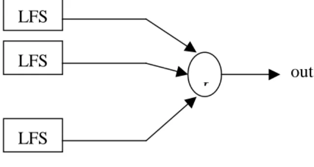
(4) Ri (2 Li − 1) possibilities for the LFSRi part of. there are Fact. The linear complexity of the keystream generated by a nonlinear filter generator with a LFSR of length L and a filtering function f of nonlinear order m is at most m.  L. ∑  i  . i =1. the key and the total number K of the keys for the pseudo-noise generator in Figure 2.4 is m. K = Π Ri (2 Li − 1) . i =1.  . Adding a filter function to a LFSR may increase the linear complexity of the output sequence, but the period is at most still the same. Another general technique for destroying the linearity inherent in LFSRs is to generate the keystream by a nonlinear function F of the outputs of several LFSRs. Figure 2.4 shows the structure. The kind of keystream generator is called a nonlinear combination generator and the function F is called the combining function.. In a brute force attack and a worst case situation, all of the K keys have to be examined, which is not feasible. However, there may be correlation between some of the inputs Si and the output Z. T. Siegenthaler [7] proposed a divide and conquer correlation attack method that the LFSRi part of the key would be found independently from. ( j = 1, ..., m ; j ≠i ) with approximately Ri ( 2 − 1) tests. So, the number of trials. the. LFSRj. parts. Li. m. can be reduced from. Π R (2 i =1. LFS. m. Σ R (2. LFS F. out. LFS Figure 2.4.. A combination generator. Every Boolean function F(x1,x2,…,xm) can be written as a modulo 2 sum of distinct mth order products. The expression is called the algebraic normal form of F.. Fact. Suppose that m LFSRs, whose lengths L1, L2, …, Lm are pairwise distinct and greater than 2, are combined by a nonlinear function F(x1,x2,…,xm) which is expressed in algebraic normal form. The linear complexity of the keystream is F(L1,L2,…,Lm).. 3. Correlation Attacks. i =1. i. L. φ(2 Li − 1) polynomials for an LFSR equals . Hence, Li. − 1) to approximately. − 1) .. The model is also the commonest type of keystream generators that consist of m LFSRs whose output sequences are combined by a nonlinear function F. Let the correlation probability between the output sequence z of the keystream generator and the output sequence a of a LFSR be larger than 0.5 . Suppose that N digits of the output sequence z of the combining function are given, the feedback connection polynomial of the LFSR with t taps and length L is known, and the LFSR generates a sequence a.. z F. ..... length Li has 2 i − 1 different possible initial states and the number Ri of different primitive feedback connection. Li. A few correlation attack methods were proposed after T. Siegenthaler showed that it is possible to independently reconstruct the initial state of each LFSR combined by a combining function with the divide and conquer correlation attack method if there exists a measure of correlation between the keystream sequence and the outputs of the LFSRs. In 1988, a fast correlation attack using parity check equations was proposed by Willi Meier and Othmar Staffelbach [8][9].. In conventional cryptography, pseudo-noise generators ( pn-generators ) consist of m linear feedback shift registers of length Li ( i = 1 , 2 , … , m ) and a known combining function F ( see Figure 2.4 ). To avoid a cryptanalytic attack using Berlekamp-Massey algorithm, the combining function F should be nonlinear. The initial state and feedback connection polynomial of LFSRi are referred to as the LFSRi part of the key. Assume that the feedback connection polynomials of all LFSR’s of length Li ( i = 1, 2, …, m ) are primitive. So LFSRi of. Li. i. LFS. a Figure 3.1.. p = Pr( zn = an ). A model of Meier-Staffelbach algorithm. By iterated squaring of the feedback connection polynomial of the LFSR, an amount of linear relations will be generated for every digit an, and each relation contains 4.

(5) t+1 digits of the sequence a. For example, the feedback connection polynomial c(x) with 2 taps of a LFSR of. x 4 + x 3 + 1 , then we know a linear relation a n = a n −3 + a n− 4 . By shifting the index, we can get the other two linear relations a n + 3 = a n + a n −1 and a n + 4 = a n +1 + a n that contain an. Using the fact that in. =. equations i.e. ( x + x + 1 )2 = x + x + 1 is also a polynomial of weight t+1. Therefore, we can generate t+1 parity check equations for a fixed position an. 4. 3. 8. 6. The average number m of the relations can be computed as. m = m( N , L, t ) = (t + 1) ⋅ log 2 (. N ) . 2L. Thus for a fixed position an, we can write the m relations as an + b1 = 0 , an + b2 = 0 , . . . , an + bm = 0 where each bi is the sum of t other different positions of the sequence a. Applying the same relations to the corresponding positions of the keystream z, we also get m relations as. m i. i =h. length 4 is. GF(2), c(x)j = c(xj) for j = 2i, we can get more parity check. ∑( m. ) p s (1 − s) i. m −i. T(p,m,h) = Pr( zn = an | at least h out of the m relations are satisfied Li = 0 ) = R(p,m,h) / Q(p,m,h) Since p > 0.5 and t is even, as h grows, p* grows, that is, the probability of zn = an increases. Thus the idea of Meier and Staffelbach is proved valid. We want to choose enough digits of sequence z to reconstruct the sequence a, hence we have to determine the maximum value of h such that Q(p,m,h)．N ≧ L. After deciding the value of h, we search for the digits of the sequence z which satisfy at least h parity check equations as a reference guess I0 of the sequence a at the corresponding positions to reconstruct the sequence a by the relations. We can also estimate the average number r of errors of I0 by. r = ( 1 − T( p, m, h) ) •L . If r << 1, these digits are likely correct. We can examine whether the initial state we calculate from I0 is correct by computing correlation and comparing it with the threshold which we describe in the previous section. If it is wrong, find the correct guess by testing modifications of I0 which has Hamming distance 1, 2, … until a correct one is obtained. 4. Improve the Meier-Staffelbach Algorithm. zn + y1 = L1 , zn + y2 = L2 , . . . , zn + ym = Lm where each yi is the sum of t other different positions of the sequence z. The idea of Meier and Staffelbach is that the more parity check equations of zn held, the higher is the probability of zn = an. Then we use the digits of the sequence z which are likely to be same with the corresponding digits of the sequence a to reconstruct the sequence a. And the initial state of the LFSR is figured out. We know that the probability p = Pr( zn = an ) and s = Pr( yi = bi ) = s(p,t) can be computed from the recursion: s(p,t) = p s(p,t-1) + (1-p)(1-s(p,t-1) ) , s(p,1) = p, we can calculate these probability variables :. Although Meier-Staffelbach algorithm is efficient, there are still some defects. We will discuss these defects and propose improvements to lower the influence caused by these defects.. Defect 1.. The number t of the taps should be small.. First, let’s consider the probability Pr( yi = bi ). It can be computed from the recursion: Pr( yi = bi ) = s = s(p,t) = p s(p,t-1) + (1-p)(1-s(p,t-1) ) and s(p,1) = p. By the recurrence relation, we can solve s:. s ( p, t ) − (2 p − 1) s ( p, t − 1) = 1 − p. *. p = Pr( zn = an | exactly h out of the m relations are satisfied Li = 0 ). ps h (1 − s ) m − h = ps h (1 − s ) m − h + (1 − p)(1 − s ) h s m − h Q(p,m,h) = Pr( at least h out of the m relations are satisfied Li = 0 ). =. ∑( ) ( m. i =h. m i. p s (1 − s ) i. m −i. + (1 − p )(1 − s ) s i. m −i. ). R(p,m,h) = Pr( zn = an ∩ at least h out of the m relations are satisfied Li = 0 ). ( 2 p − 1) [ s ( p , t − 1) − ( 2 p − 1) s ( p , t − 2 ) ] = ( 2 p − ：：. ：：. ( 2 p − 1 ) t − 2 [ s ( p , 2 ) − ( 2 p − 1 ) s ( p ,1 ) ] = ( 2 p. s ( p , t ) − ( 2 p − 1) t −1 s ( p ,1) = (1 − p ) [1 + ( 2 p − 1) + ... +. 5.

(6) = (1 − p ). 1 − (2 p − 1) t −1 1 − (2 p − 1)t −1 = 1 − (2 p − 1) 2. By iterated squaring of the connection polynomial, we have only three parity check equations:. c( x ) = x 5 + x 4 + x 3 + x 2 + 1. 1− (2 p −1)t−1 1+ (2 p −1)t ⇒ s( p, t) = (2 p −1) ⋅ p + = 2 2 t −1. So, if t is too large, the probability Pr( yi = bi ) = s(p,t) will approximate to 0.5 and p* =. .. ,. (c( x) ) = x + x + x + x + 1 (c( x) )4 = x 20 + x16 + x12 + x8 + 1 2. 10. 8. 6. 4. and ,. that. mean. a n + a n+1 + a n + 2 + a n + 3 + a n + 5 = 0 , a n + a n + 2 + a n + 4 + a n+ 6 + a n +10 = 0 and a n + a n + 4 + a n +8 + a n +12 + a n + 20 = 0 respectively. But. psh (1− s)m−h p(0.5)h (0.5)m−h there are still many weight-5 parity check equations like ≈ =p psh (1− s)m−h + (1− p)(1− s)h s m−h p(0.5)h (0.5)m−h + (1− p)(0.5)h (0.5)m−h a + a + a + a + a = 0 , … etc. And there n. exists. This means that no matter how many parity check equations of a digit are held, the probability p* approximates to a constant p = Pr( zn = an ) if t is too large. Therefore the probability p* doesn’t give us more information than the probability Pr( zn = an ) such that Meier-Staffelbach algorithm becomes an exhaustive search.. Besides, when we want to determine the value of a certain digit, we need to find a parity check equation which contains the digit and another t digits believed to be correct. So it is infeasible if t is large.. Defect 2.. N should be neither too small nor too large. L. From the formula that if. m = (t + 1) ⋅ log 2 (. N ) , we know 2L. N is too small, the number of parity check L. equations we can get by iterated squaring of the connection polynomial would be small such that the accuracy probability of the digits which have the most parity check equations held would be low.. n +1. n+5. even. weight-3. n+6. n+9. parity check equations like a n + a n +3 + a n +8 = 0 , ,. an + an +1 + an +12 = 0 a n + a n+ 5 + a n + 28 = 0 , and etc.. Hence W. T. Penzhorn [11][12] proposed a long division algorithm to compute low-weight parity check equations. Suppose that the connection polynomial of the LFSR of length L is c(x) and the number of digits of the LFSR’s output sequence a we observe is N, and N ≦ 2L-1 . We want to compute some parity check equations of weight w. For example, given the connection polynomial c(x) = x4 + x + 1, we want to compute weight-3 parity check equations, and choose ν max = 14 . When j = 13, we obtain a. x14 + x13 + x 2 is a parity check equation and a n + a n +1 + a n +12 = 0 . remainder x2 which is a single term. So. When j = 12, we also obtain a parity check equation. x14 + x12 + x a n + a n+ 2 + a n +9 = 0 .. which. If w > 3, we may obtain more than one parity check equation in the Step 3 each round. In the above example, if we want to compute weight-4 parity check equations, and choose νmax = 14, we obtain. If N is too large, the number Q(p,m,h)．N ≈ L of the digits that we believe to be correct is small relatively. There may be not enough relations among these reference digits to determine the whole sequence a and the initial state of the LFSR. Meier-Staffelbach algorithm requires the number t of taps of the connection polynomial to be small – typically less than 10 . Even t is small, there may exist some parity Step 3. check equations with weight t+1 or less than t+1, but we can’t get them by iterated squaring of the connection polynomial. For example, suppose that the connection polynomial of a LFSR is. c( x) = x 5 + x 4 + x 3 + x 2 + 1 . It is primitive and the period of the output sequence of the LFSR is 25 - 1 = 31 .. means. x14 + x13 + x11 + x 9 and. x14 + x13 + x 6 + x 5 when j = 13 . Compute Weight-3 Parity Check Equations Since there exists at most one i such that x max + x + xi is a parity check equation, if we want to compute weight-3 parity check equations, Step 3 of Penzhorn’s long division algorithm can be modified as follows. ν. Use long division to divide single-term remainder νmax. x. j. xνmax + x j by c(x) until a xi. is. obtained.. And. + x + x is a parity check equation. j. i. However Penzhorn’s long division algorithm is not efficient to compute weight-3 parity check equations. If we 6.

(7) make some preparations, we can speedily determine the value of i if there exists such an i ≦ N.. Each digit an can be expressed as a linear combination of S1 ~ S L : the initial state. a n = e1,n S1 + e2, n S 2 + ... + e L , n S L . And ei,n is the nth output digit of the LFSR with the initial state of all 0’s except Si = 1 . Therefore, the coefficients. e1,n , e2,n , ..., e L ,n can be determined easily. If xνmax + x j + x i is a parity check equation, then an + an +νmax − j + an+ν max −i = 0 and ed,n + ed,n +νmax − j + ed,n +ν max −i = 0 for 1≦d≦N. As long as we record and sort all n ≦. < e1,n , e2, n , ..., eL ,n > for. N in preparation, when given a set of. < e1,i , e2,i , ..., eL ,i > , we can speedily search for the value of i or determine whether there exists such i ≦ N using binary search in time complexity O(logN). The formula. m = (t + 1) ⋅ log 2 (. N ) is to calculate 2L. the ‘average’ number of the relations of each digit. Many digits have more than. (t + 1) ⋅ log 2 (. N ) relations. The 2L. maximum value of h which satisfies Q(p,m,h)．N ≧ L is usually too small such that the number of the reference digits which have at least h parity check equations held is much more than L. Therefore, in practice we should not adopt the value of h from the above formula, and we distinctly count the number of held parity check equations of each digit, and then determine the maximum value of h such that the number of digits which have at least h parity check equations held is equal to or greater than L. Let’s look at the result of a simulation program to compare the modified version with the original Meier-Staffelbach algorithm. We set the probability Pr( zn = an ) = 0.75 and the connection polynomial. c( x) = x100 + x 37 + 1 which is primitive, and decide to observe 20,000 digits. The program randomly chooses an initial state, calculates the 20,000-digit output a of the LFSR and the combining function’s 20,000-digit output sequence s which is correlated to a with a probability 0.75, and then counts and records the number of parity check equations held of each digit. We run the program 10,000 times and we found we got better results. Due to the limited space the results are not shown here. In the original Meier-Staffelbach algorithm, according to the formula m =. ( t + 1) ⋅ log. 2. (. N ) , the 2L. maximum value of h which satisfies Q(p,m,h)．N ≧ L is 16 .. algorithm chooses all correct reference digits in only 917 times of 10,000 simulations because the value of h we determine is too small such that we choose too many digits as the reference digits. The modified Meier-Staffelbach algorithm chooses all correct reference digits in 9,798 times of 10,000 simulations. The modified Meier-Staffelbach algorithm we proposed chooses fewer digits as the reference digits to prevent from error digits. But it isn’t always successful to calculate the initial state from the relations among the reference digits. For example, suppose that the connection polynomial is c(x) = x7 + x + 1 . We observe 127 digits of the output sequence z of the combining function: 011111010110001000111011100000000111111000100101 010011001000000111000110111110011101000110110001 0011100001011000110000010100110 . By iterated squaring of the connection polynomial, we know these parity check equations: a n + a n+ 6 + a n + 7 = 0 , a n + a n+12 + a n +14 = 0 , a n + a n+ 24 + a n + 28 = 0 , a n + a n+ 48 + a n + 56 = 0 and a n + a n +96 + a n +112 = 0 . Only z104 has 11 relations held. No digit has more than 11 relations held. And z 55 , z 65 , z 68 , z 76 , z100 , z105 and z113 have 10 relations held respectively. Then we choose these digits and determine the corresponding positions ( a 55 , a 65 , a 68 , a 76 , a100 , a105 and a113 ) of the output sequence a of the LFSR as a reference. Although we choose more than 7 digits, only a 20 , a 57 , a 98 , a121 , a90 , a 43 and a86 can be calculated from the relations of the reference digits. Therefore, in this case, the initial state cannot be determined by the modified Meier-Staffelbach algorithm. As we discuss before, each digit an can be expressed as a linear combination of the initial state S1 ~ S L :. a n = e1,n S1 + e2, n S 2 + ... + e L , n S L . It is known that a system of L independent linear equations in L unknowns can be solved. Hence if we select L independent digits of the sequence a, we are able to solve S1 ~ S L directly by Gaussian elimination rather than calculating the whole sequence a to determine S1 ~ S L by the relations. On the contrary, if less than L independent digits are selected, we cannot determine S1 ~ S L exactly and have to guess some of them. And if we select some dependent but wrong digits, the system of linear equations may have no solution. With the concept, we know that the key point of choosing digits is not to enlarge the number of chosen digits but to select enough ( at least L ) independent digits. And we should be able to calculate the value of a digit from the digits those are dependent with it. Hence, superfluous dependent digits are not only useless for solving the system of linear equations but may also hamper the system from having solution. Our improved algorithm is then as follows.. In our simulation result, the original Meier-Staffelbach 7.

(8) with controllable complexity,” IEEE Transactions on Information Theory, Vol. IT-17, No. 3, May. 1971, pp. 288-296.. Step 1. Calculate the number of parity check equations held of each digit. Step 2.. Step 3.. Step 4.. Determine the coefficients e1,n , e2,n , ..., eL,n of each digit an’s linear combination of the initial state S1 ~ S L . According to the number of parity check equations held of each digit, we select L independent digits of the sequence z with relations held decreasingly. Use these digits as a reference guess I0 of the sequence a at the corresponding positions. Then solve the system of L independent linear equations to determine S1 ~ S L . Find the correct guess by examining modifications of I0 having Hamming distance 0, 1, 2, …, by the correlation between the sequence and the output sequence of the LFSR with the initial state we calculated.. 5. Conclusions In this paper, we discuss the requirements of a keystream generator in a stream cipher system and the structure and properties of an LFSR. The output sequence of an LFSR has a large period and is unpredictable. But it is easy to attack a LFSR using Berlekamp-Massey algorithm. So most stream cipher systems adopt the nonlinear combination generators that consist of several LFSRs. Correlation attacks are the most popular methods used to attack a stream cipher system. Willi Meier and Othmar Staffelbach proposed a fast correlation attack method using parity check equations. An important design criterion requires that there should be very low correlation between the keystream of the combining function and the output sequence of an arbitrary LFSR of short length otherwise Meier-Staffelbach algorithm could be used to attack the stream cipher system. We show that it is easy to find low-weight parity check equations no matter how many taps of the LFSR are. In particular, all weight-3 parity check equations, if exist, can be obtained. We also adopt another strategy to choose digits as a reference. Viewing each output digit of the LFSR as a linear combination of the initial state, we choose exactly L independent and most likely correct digits, and solve the system of linear equations to determine the initial state rather than calculating the whole output sequence and the initial state of the LFSR from the relations among the reference digits. Therefore, our algorithm can avoid the situation where the reference digits are not enough to calculate the initial state in Meier-Staffelbach algorithm.. [3] Abraham Lempel, “Analysis and synthesis of polynomials and sequences over GF(2),” IEEE Transactions on Information Theory, Vol. IT-17, No. 3, May. 1971, pp. 297-303. [4] Abraham Lempel, and Jacob Ziv, “On the complexity of finite sequences,” IEEE Transactions on Information Theory, Vol. IT-22, Jan. 1976, pp. 75-81. [5] Edwin L. Key, “An analysis of the structure and complexity of nonlinear binary sequence generators,” IEEE Transactions on Information Theory, Vol. IT-22, No. 6, Nov. 1976, pp. 732-736. [6] T. Siegenthaler, “Correlation-immunity of nonlinear combining functions for cryptographic application,” IEEE Transactions on Information Theory, Vol. IT-30, No. 5, Sep. 1984, pp. 776-780. [7] T. Siegenthaler, “Decrypting a class of stream ciphers using ciphertext only,” IEEE Transactions on Computers, Vol. C-34, Jan. 1985, pp. 81-85. [8] Willi Meier, and Othmar Staffelbach, “Fast correlation attacks on stream ciphers,” Advances in Cryptology-EUROCRYPT’88, Lecture Notes in Computer Science, Vol. 330, Springer-Verlag, 1988, pp. 301-314. [9] Wille Meier, and Othmar Staffelbach, “Nonlinearity criteria for cryptographic functions, ” Advances in Cryptology-EUROCRYPT’89, Lecture Notes in Computer Science, Vol. 434, Springer-Verlag, 1989, pp. 549-562. [10] Kencheng Zeng, Chung-Huang Yang, Dah-Yea Wei, and T.T.N. Rao, “Pseudorandom bit generators in stream-cipher cryptography,” Computer, Vol. 24, Feb. 1991, pp. 8-17. [11] W. T. Penzhorn, “Correlation attacks on stream ciphers: computing low-weight parity checks based on error-correcting codes,” Fast Software Encryption, FSE’96, Lecture Notes in Computer Science, Vol. 1039, 1996, pp. 145-158. [12] W. T. Penzhorn, “Correlation attacks on stream ciphers,” AFRICON, 1996., IEEE AFRICON 4th, Vol. 2, 1996, pp. 1093-1098. [13] Solomon W. Golomb, Shift register sequences, Holden-Day, 1967. [14]. Douglas R. Stinson, Cryptography : theory and practice, CRC Press, 1995.. [15]. Bruce Schneier, Applied cryptography second edition : protocols, algorithms, and source code in C, John Wiley & Sons, 1996.. REFERENCES [1]. J. L. Massey, “Shift-register synthesis and BCH decoding,” IEEE Transactions on Information Theory, Vol. IT-15, 1969, pp. 122-127.. [16]. Alfred Menezes, Paul van Oorschot, and Scott Vanstone, Handbook of applied cryptography, CRC Press, 1997.. [2]. Edward J. Groth, “Generation of binary sequences. [17]. Thomas W. Cusick, Cunsheng Ding, and Ari 8.

(9) Renvall, Stream ciphers and number theory, Elsevier Science B.V., 1998.. 9.

(10)